www.nonlin-processes-geophys.net/14/31/2007/ © Author(s) 2007. This work is licensed under a Creative Commons License.
Nonlinear Processes
in Geophysics
Models for strongly-nonlinear evolution of long internal waves in a
two-layer stratification
T. Sakai and L. G. Redekopp
Department of Aerospace & Mechanical Engineering, University of Southern California, Los Angeles, CA 90089-1191, USA Received: 1 June 2006 – Revised: 19 January 2007 – Accepted: 26 January 2007 – Published: 30 January 2007
Abstract. Models describing the evolution of long internal waves are proposed that are based on different polynomial approximations of the exact expression for the phase speed of uni-directional, fully-nonlinear, infinitely-long waves in the two-layer model of a density stratified environment. It is argued that a quartic KdV model, one that employs a cubic polynomial fit of the separately-derived, nonlinear relation for the phase speed, is capable of describing the evolution of strongly-nonlinear waves with a high degree of fidelity. The marginal gains obtained by generating higher-order, weakly-nonlinear extensions to describe strongly-weakly-nonlinear evolu-tion are clearly demonstrated, and the limitaevolu-tions of the quite widely-used quadratic-cubic KdV evolution model obtained via a second-order, weakly-nonlinear analysis are assessed. Data are presented allowing a discriminating comparison of evolution characteristics as a function of wave amplitude and environmental parameters for several evolution models.
1 Preliminary considerations
The wide-spread appearance of packets of long internal waves in the shallow, stratified waters of the coastal ocean and lakes is firmly established (Osborne and Burch, 1980; Apel et al., 1985; Scotti and Pineda, 2004; Ostrovsky and Stepanyants, 1989; Stanton and Ostrovsky, 1998; Antenucci et al., 2000; Duda et al., 2004; Helfrich and Melville, 2006). These long-wave packets in many contexts are decidedly nonlinear, containing waves with amplitudes that are equal to and greater in magnitude than the controlling length scale of the problem, which is typically the scale of the upper-mixed layer depth. Furthermore, these long-wave packets are known to stimulate strong benthic dissipation and mix-ing, having a determining influence on the decay of internal Correspondence to: T. Sakai
tidal energy and the resuspension and transport of sedimen-tary material (Bogucki et al., 1997; Bogucki and Redekopp, 1999; Stastna and Lamb, 2002; Bogucki et al., 2005). Hence, there is increasing interest in the development of models that can yield quantitative, evolutionary descriptions of such wave packets in a wide range of environments. The present work is directed toward proposing such a model, and assess-ing its potential (along with that of various alternate models) to describe reliable descriptions of packets possessing large amplitude internal waves.
Aspects of the propagation of nonlinear internal waves in the long-wave limit are examined in the case of a two-layer model under the Boussinesq approximation. Specifically, uni-directional propagation of a plane wave is considered in the idealized environmental model of a two-layer density stratification. This idealized case represents a convenient and quantitatively relevant model for the lowest internal wave mode in realistic stratifications when the water column pos-sesses a single, prominent, thermoclinic layer whose depth is at most a modest fraction of the fluid depth. In what fol-lows, the characteristics of the environmental model are de-fined in terms of the undisturbed, upper (lower) layer depths
h1(h2) and respective fluid densitiesρ1(ρ2), and the inter-face displacement is denoted by the functionζ (x, t ). Within the Boussinesq approximation the layer densities enter only through the reduced gravityg˜=g(ρ2−ρ1)/ρ1.
ζt+c0(1−α1ζ−α2ζ2)ζx+β0c0ζxxx =0. (1)
In the terminology adopted here this equation is referred to as KdV2 whenα26=0, and as KdV1 whenα2=0. KdV1 is the familiar and widely-studied equation where the nonlinearity derives solely from the leading-order, nonlinear correction to the linear long-wave phase speed c0. KdV2 represents the case where both the first-order and second-order depen-dencies (i.e., linear and quadratic terms in an asymptotic ap-proximation for small amplitudes) of the long-wave phase speed on wave amplitude are incorporated into the evolution model. The coefficients in this equation have the following representations in terms of the layer depths for the two-layer environmental model:
c20= gh˜ 1h2 h1+h2
= 1
2gh(˜ 1−
2); (2)
α1= 3 2
h2−h1 h1h2
= 3
h(1−2)≡ ˜ α1
h ; (3)
α2= 3 8
(h2−h1)2+8h1h2 (h1h2)2
=3
2
2−2 h2(1−2)2 ≡
˜ α2 h2; (4) β0=
1 6h1h2=
1 6h
2(1−2). (5)
These coefficients are given in two different forms, the latter obtained by using the alternate representationsh1=h(1−), h2=h(1+)for the layer depths withhequal to one-half the fluid column depth and=(h2−h1)/2h.
The fact that the coefficients of various terms in the evo-lution Eq. (1) are available in terms of analytical expressions that are easily calculated makes the two-layer model attrac-tive for first-order estimates of wave properties. Neverthe-less, a nagging question relating to any asymptotic approxi-mation is the quantitative utility of representing a nonlinear function in terms of only the leading terms of its asymptotic expansion. This has been a persistent concern regarding the application of KdV theory in contexts where there is a com-pelling interest in assessing or comparing physical character-istics at a quantitative level (e.g., front propagation speeds, wave profile shapes, local wave-induced velocity shear and mixing, wave-induced benthic stimulation, vertical and hor-izontal particle transport by a solitary wave or long-wave packet, etc.).
2 The case of equal layer depths
The first issue to be addressed is the evolution of the inter-facial wave in the limiting case when the layer depths are nearly equal, and when the wave amplitude becomes large. When=0 one observes from Eqs. (3) and (4) thatα1=0 and α2=3/ h2. In this limiting situation we have a special case of KdV2 and, as noted originally by Djordjevic and Redekopp (1978), both α2>0 and β0>0 so that nonlinear steepening
augments the effect of linear dispersion and no equilibrium solutions (e.g., solitary waves) are possible. Also, the evolu-tion equaevolu-tion has the invarianceζ→−ζ and a waveform of either polarity is possible. This is in contrast to the leading order case for disparate depths (i.e., when|α1||α2ζ| and the evolution is essentially described by KdV1). Equilibrium solutions of KdV1 are possible whenα1ζ andβ0 have op-posite signs, a condition implying that the wave polarity is always such that the interface displacement is a wave of ele-vation with respect to the shallowest layer.
The key point relating to this first issue is the sign (and magnitude) of the higher-order terms in Eq. (1) whentends toward zero, either from positive or negative values. That is, althoughα1tends to zero with, what are the sign and mag-nitude ofα3, etc., for small values of||. The issue is readily addressed through use of a recent result by Slunyaev et al. (2003) where, based on earlier work by Ostrovsky and Grue (2003), an analytic expression for the fully-nonlinear, long-wave propagation speed for a long-wave moving in one direction was derived (see Eq. 45 in Ostrovsky and Stepanyants, 2005):
˜ cE=
cE c0
=1+3 h2−h1
(h1+h2)2
(h2−h1+2ζ )× (s
(h1−ζ )(h2+ζ ) h1h2
−h2−h1+2ζ h2−h1
)
=1−3(+ ˜ζ )2+3(+ ˜ζ )
s
1−(+ ˜ζ )2
1−2 . (6)
Dimensionless variables (c˜E,ζ˜)=(c/c0,ζ / h) are employed in the second representation of the expression, termed the “exact” value and denoted byc˜E. It is readily apparent, and
quite important to note, that Eq. (6) possesses the symmetry propertyc˜E(ζ˜;)= ˜cE(− ˜ζ; −).
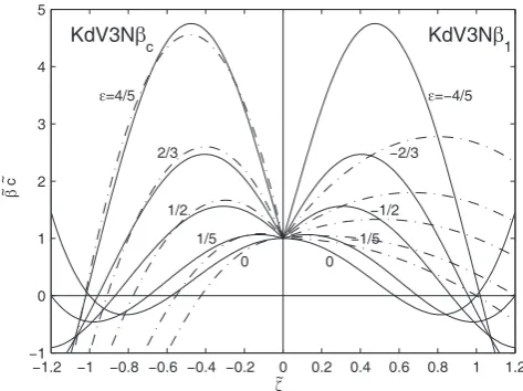
The dependence of the phase speedc˜Eon wave amplitude
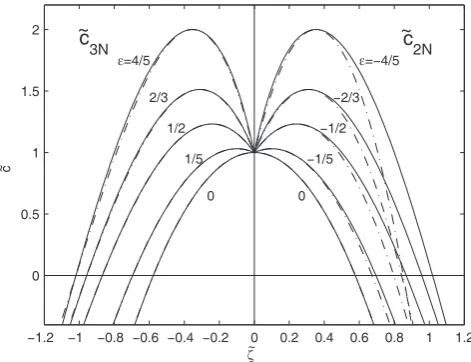
is displayed in Fig. 1 for several ratios of the layer depths (i.e., values of). Results are shown by solid lines in the figure and correspond to waves with physically relevant po-larities; that is, waves of depression (ζ <˜ 0) for>0 (h1<h2) and waves of elevation (ζ >˜ 0) for<0 (h1>h2). One ob-serves immediately that the phase speed is not a monotonic function of the wave amplitude. The negative sign before the
α2coefficient causes the long-wave phase speed to diminish as the wave amplitude increases. It is only in the particular case of equal layer depths that the phase speed is a monotonic function of the amplitude, diminishing continuously from its maximum value of unity (i.e., the linear value) as the ampli-tude increases.
−1.2 −1 −0.8 −0.6 −0.4 −0.2 0 0.2 0.4 0.6 0.8 1 1.2 0
0.5 1 1.5 2
ζ ~
c
ε=4/5 ε=−4/5
2/3 −2/3
1/2 −1/2
1/5 −1/5
0 0
c
3N 2N
~
~
~ c
Fig. 1. The exact, fully nonlinear long-wave phase speed as a func-tion of wave amplitude for various layer-depth ratios, including comparison with two polynomial fitsc˜2Nandc˜3N.
maximum value ofc˜E, and the corresponding wave
ampli-tudeζ˜
m where the phase speed maximum occurs, are also
given in Table 1. Expressions for these relations can be de-rived from the expression in Eq. (6) and their analytical forms are presented subsequently.
With Eq. (6) in hand, it is straightforward to develop the weakly-nonlinear expansion of the phase speed to orders be-yond the quadratic term (i.e., theα2 term) that appears in Eq. (1) and is defined in Eq. (4). The expansion of Eq. (6) to higher orders yields the extended expression
˜
cE =1−α1ζ−α2ζ2−α3ζ3−α4ζ4− · · ·. (7) We draw particular attention to the expressions for the fol-lowing higher-order terms:
α3= 3 16
(h2−h1)(h1+h2)2 (h1h2)3
= 3
2
h3(1−2)3 ≡ ˜ α3 h3; (8) α4=
15 128
(h2−h1)2(h1+h2)4 (h1h2)4
= 15
8
2 h4(1−2)4
≡ ˜α4/ h4. (9)
One notes thatα˜1andα˜3 (and furtherα˜i for oddi) always
carry the same sign, being proportional to=(h2−h1)/2h. However, and most significantly, all coefficientsα˜i vanish
whenh2=h1fori≥3. Consequently, and as pointed out in the note by Slunyaev et al. (2003), the expansion for the non-linear phase speed for long-wave propagation terminates at theα˜2 term when the layer depths are equal, and the fully-nonlinear phase speed whenh2=h1 is given exactly by the simple polynomial expression
˜
cE =1−3ζ˜2. (10)
Stated in another way, the well-established coefficient for the cubic KdV equation (Eq. 1 withα1=0) contains already the
Table 1. Environmental parameters and corresponding wave prop-erties for a range of depth ratios.
h2/ h1 ζ˜1 ζ˜c ζ˜max c˜Emax
0 1 ζ˜ −1/√3 0.000 1.000
1/5 3/2 5ζ /˜ 4 −0.696 −0.100 1.031
1/3 2 3ζ /˜ 2 −0.773 −0.164 1.091
1/2 3 2ζ˜ −0.868 −0.241 1.232
3/5 4 5ζ /˜ 2 −0.923 −0.284 1.375
2/3 5 3ζ˜ −0.957 −0.310 1.513
3/4 7 4ζ˜ −0.998 −0.339 1.768
4/5 9 5ζ˜ −1.019 −0.353 2.000
5/6 11 6ζ˜ −1.032 −0.361 2.214
6/7 13 7ζ˜ −1.040 −0.365 2.412
7/8 15 8ζ˜ −1.046 −0.367 2.598
8/9 17 9ζ˜ −1.050 −0.368 2.774
9/10 19 10ζ˜ −1.052 −0.369 2.941
exact nonlinear steepening when the layer depths are equal. Furthermore, and as seen in Fig. 1 and noted in Table 1, we find the surprising result that the nonlinear propagation speed diminishes to zero for wave amplitudes of either po-larity approaching the limiting value| ˜ζc|=1/
√
3. This con-sequence of waves becoming stagnant as the wave amplitude increases was observed in simulations for shoaling of wind-driven, long internal waves in a lake1, and was an initiatial motivation for the study presented here. The critical values
˜
ζc (i.e., amplitudes wherec˜E=0) for other depth ratios are
included in Table 1.
3 Strongly nonlinear long waves
The second and principal issue addressed pertains to the range of validity of the weakly nonlinear representation of the phase speed and, consequently, the specification of the appropriate “extended” evolution equation for depth ratios that are not near unity. When considering numerical simula-tions of lowest-mode, long internal wave motion along a sin-gle characteristic direction in shallow waters, the exact non-linear expressioncE(ζ )for the long-wave phase speed given
in Eq. (6) can be inserted in place of the quadratic approxima-tion appearing in Eq. (1). However, it is of some interest to have a polynomial approximation forcE(ζ )in order to obtain
an evolution equation that potentially yields analytical (i.e., parameterized) expressions for equilibrium solutions, a hier-archy of conserved densities, and yet possesses the capacity
−0.8 −0.7 −0.6 −0.5 −0.4 −0.3 −0.2 −0.1 0 0.5
1 1.5
ζ~ SN
S
1
S
3
S
2
S
4
ε=1/3
(a)
−0.8 −0.7 −0.6 −0.5 −0.4 −0.3 −0.2 −0.1 0 0.5
1 1.5
ζ~ SN
S
1
S
3
S
2
S
4
ε=2/3
(b)
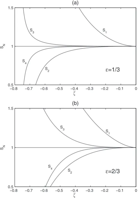
Fig. 2. Comparison of various truncations of the weakly-nonlinear approximation for the long wave phase speed with its exact expres-sionc˜E. (a)=1/3; (b)=2/3.
to reliably describe wave motions over a wide range of am-plitudes.
3.1 Higher-order approximations
Toward the objective of generating a polynomial approxi-mation for c˜E(ζ;), the truncated version of the
weakly-nonlinear expansion ofc˜E is first compared to the exact
ex-pression in terms of the following quantity:
SN(ζ˜;)=
1− N
X
k=1 ˜ αk()ζ˜k
˜ cE(ζ˜;)
. (11)
The deviation ofSN(ζ˜;)from unity measures the error
con-tained in the different truncations of the power series expan-sion, and provides a basis for defining the range of valid-ity of the widely-used KdV1 and KdV2 versions defined by Eq. (1). Values of the functionSN(ζ˜;)for several values
ofare shown in Fig. 2 for different choices of the trunca-tion parameterN. It is clear that KdV2 (i.e., theS2 curve
in Fig. 2) extends considerably the range of wave amplitudes over KdV1 (i.e., theS1 curve) where quantitative descrip-tions are sought. Nevertheless, the approximate represen-tation of the long-wave phase speed diverges quite rapidly from the true nonlinear value at wave amplitudes that may be well below those observed in a number of contexts. One al-ternative to extending the weakly-nonlinear expansion ofc˜E
to be used in the evolution equation, without resorting to an excessively high order truncation of the series representation forc˜E(ζ˜;), is to seek some approximate summation of the
series. To this end, the power-series expansion of the expres-sion in Eq. (6) has been developed to high order and arranged in the following form:
˜
cE=1− ˜α1ζ˜− ˜α2ζ˜2 − ˜α3ζ˜3
1+5
4
˜ ψ+3
2
˜ ψ2+7
4
˜
ψ3+2ψ˜4+ · · ·
+1
4
˜ φ
1+7
2
˜
ψ+8ψ˜2+16ψ˜3+ · · ·
+1
8
˜ φ2
1+45
8
˜ ψ+ · · ·
+ · · ·
. (12)
The quantities (ψ˜,φ˜) appearing in this expression are defined as
˜
ψ=
˜ ζ
1−2; ˜ φ=
˜ ζ2
(1−2)2. (13)
Examination of this series suggests that any practical trunca-tion ofc˜Ein polynonnmial form must include a term of order
˜
ζ3. With this in view, and motivated by the desire to produce an evolutionary model with polynomial nonlinearity, we pro-pose using the “summed-series”c˜S for the nonlinear phase
speed
˜
cS=1− ˜α1ζ˜− ˜α2ζ˜2− ˜α3Sζ˜3, (14)
yielding the extended evolution equation, termed here as KdV3S, with a quartic nonlinearity.
The coefficient α˜3S of the quartic nonlinear term in
Eq. (14) is a “modeled” version of the coefficientα˜3, a modi-fication toα˜3that is designed to capture in approximate form the higher-order terms in Eq. (14) forc˜E(ζ˜;). The modeled
expression forα˜3Sis
˜ α3S =
3 2
(1−2)3exp
(
−KS |ζ˜S|
1−2 )
×
exp
( ˜
ζS2
(1−2)2 )
, (15)
which is obtained via a “pivoting” of the summed portion of the infinite series about a selected value of the wave ampli-tude, noted here asζ˜S. The different series in Eq. (12) have a
structure reminiscent of the exponential function, albeit with coefficients that clearly do not decay as 1/n!. A factorKS
for the different series involvingψ˜ terms. After some testing
of different parametric choices, a recommended set of values for the two parameters are ζ˜
S=1/3 andKS=7/3. Clearly
these choices are somewhat arbitrary, and alternate values may yield a better fit for any given value of, yet we sug-gest that the selected values yield a “respectable fit” encom-passing a significant and physically-relevant range of depth ratios. The modeled form c˜S(ζ˜;)of the phase speed for
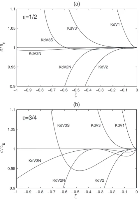
two depth ratios over a range of wave amplitudes is shown in Fig. 3 by the curve noted as KdV3S. Results in Fig. 3 are presented as a ratio of a particular approximation for the nonlinear phase speed divided by the exact valuec˜E. Hence,
departures from unity provide an immediate measure the rel-ative merits of any modeled approximation, and the range of amplitudes where its representation of the true nonlinear steepening is reasonably captured. The modeled expression
˜
cS, with its selected fit parameters, significantly extends the
range of amplitudes where a polynomial expression provides a good representation for the nonlinear steepening effects over that of KdV2, for example, but the fidelity of the fit degrades as the value ofincreases toward unity.
3.2 A full-range, quadratic approximation – KdV2N Another approach toward developing an evolution model ca-pable of describing strongly nonlinear long waves with rea-sonable fidelity, yet possessing polynomial nonlinearity is to construct a quadratic fit to the fully-nonlinear relation for
˜
cE(ζ , )˜ . To this end certain characteristic points on the
curve representing the true function can be identified, and then a limited polynomial is proposed that passes through these points, thereby providing an approximate representa-tion encompassing a wide range of wave amplitudes. The specific points vital to characterizing the functionc˜E(ζ , )˜
are the following: the intercept value (c˜E=1,ζ˜=0), the
max-imum value (c˜E= ˜cEm, ζ˜= ˜ζm), and the zero-crossing value
(c˜E=0,ζ˜00). Using Eq. (6), the following quantities can be derived:
˜
cm=1+2Sc(), Sc()=
3 2 h
1−2+p1−2i−1; (16) ˜
ζm= −Sm(),
Sm()=1−
1
√
2 h
1+p1−2i−
1 2
; (17)
˜
ζ00= −sgn()S00(),
S00()= || + 1
√
3 "
1+ 2
2 − 1 2
p
82+4 #12
. (18)
A quadratic approximation can only enforce passage through two points on the true function. Since the approximation should apply for all values of, including=0, we choose for the two pairs of (c˜E,ζ˜), the intercept value (1,0) and the
max-−1 −0.9 −0.8 −0.7 −0.6 −0.5 −0.4 −0.3 −0.2 −0.1 0 0.9
0.95 1 1.05 1.1
ζ
~
c / c
E
ε=1/2
KdV3N
KdV3
KdV2N KdV2
KdV1
KdV3S
(a)
−1 −0.9 −0.8 −0.7 −0.6 −0.5 −0.4 −0.3 −0.2 −0.1 0 0.9
0.95 1 1.05 1.1
ζ~
c / c
E
ε=3/4
KdV3N
KdV3
KdV2N KdV2
KdV1 KdV3S
(b)
~ ~
~ ~
Fig. 3. Comparison of the various polynomial approximations for the phase speed underlying the different evolution models. (a) =1/2; (b)=3/4.
imum value (c˜Em,ζ˜m). This leads to the following quadratic
fit, termedc˜2N, ˜
c2N =1− ˜κ1ζ˜− ˜κ2ζ˜2, (19) where the coefficientsκ˜1andκ˜2have the values
˜ κ1=2
Sc() Sm()
, (20)
˜ κ2=
Sc()
S2
m()
. (21)
−1.2 −1 −0.8 −0.6 −0.4 −0.2 0 −0.15
−0.1 −0.05 0 0.05 0.1 0.15
ζ
~
c3N
− c
E
2/3 3/4 4/5
ε=7/8
~ ~
Fig. 4. The phase speed error for the KdV3N model relative toc˜E for different depth ratios.
does not provide advantages over KdV3S except that it is a lower order polynomial approximation.
3.3 A full-range, cubic approximation – KdV3N
Examination of the quadratic fit exhibited on the right-hand side of Fig. 1 shows that the fidelity of the quadratic represen-tation forc˜E(ζ˜;)degrades significantly at large amplitudes
and higher values of, and that a reasonably faithful approx-imation requires at least a polynomial of cubic order. To this point, we propose a cubic approximation that, in addition to passing through the points included in defining the quadratic fit (Eq. 19), includes enforcement of the zero-crossing value (c˜E=0,ζ˜00). This leads to the approximate relation, denoted byc3N,
˜
c3N =1− ˜γ1ζ˜− ˜γ2ζ˜2− ˜γ3ζ˜3, (22) where the coefficientsγ˜iare given by the following functions
of:
˜ γ1=
S00
Sc Sm
(2S00+ ||Sm)
−|| S 2
m(1+2Sc) (S00− ||Sm)2
)
, (23)
˜ γ2=
1
S00 S
c S2
m
(S00+2||Sm)
−2|| Sm(1+ 2S
c)
(S00− ||Sm)2
)
, (24)
˜
γ3=sgn() Sc S00Sm2
( 1− S
2
m(1+2Sc) Sc(S00− ||Sm)2
)
. (25)
This cubic fit is shown by the dash-dot curves on the left-hand side of Fig. 1. The match of this cubic fit with the true
function appears remarkably good. The ratio of this approxi-mation to the true function is depicted by the curves denoted KdV3N in Fig. 3. The reader will note that the ratioc˜3N/c˜E
does not pass through the zero-crossing pointζ˜
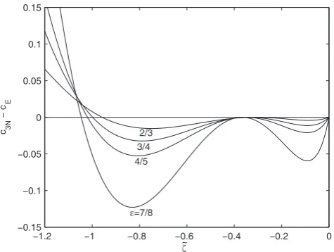
00. This oc-curs because the cubic approximation cannot enforce a si-multaneous matching of the value of the functions and their slopes at the zero-crossing point, and consequently the ra-tio is necessarily finite atζ˜00. However, in order to portray the high fidelity of the cubic approximation over the whole range of relevant wave amplitudes we present the difference between these functions 1c˜3N E (defined as the difference
˜
c3N− ˜cE) in Fig. 4 for a wide range of depth ratios.
3.4 A full-range, cubic approximation with nonlinear dis-persion – KdV3Nβ
Thus far the proposed models for strongly nonlinear evolu-tion have neglected nonlinear dispersive effects. Following Ostrovsky and Grue (2003), nonlinear dispersion can be in-corporated, at least in a modeling sense, by replacing the fixed ambient depths of the two layers with their local val-ues in the linear expression for the first dispersive correction, and by replacing the constant value of the linear, long-wave phase speedc0by its nonlinear, amplitude-dependent expres-sion c˜E(ζ )˜ . That is, the fully-nonlinear evolution of long
waves along a single characteristic can be written as
ζt +c0c˜E(ζ )ζ˜ x+β0c0
˜
β(ζ )˜ c˜E(ζ )ζ˜ xx
x
=0, (26) withc˜Egiven by Eq. (6) andβ˜given by
˜
β(ζ )˜ = (h1−ζ )(h2+ζ ) h1h2
=1−(+ ˜ζ ) 2
1−2 . (27)
The functional dependence of the productD˜E= ˜βc˜E on the
local displacement ζ˜ is somewhat complicated, having the form shown in Fig. 5. As argued further in the next sec-tion, it is of some interest to representD˜Eby an approximate
quadratic dependence onζ˜. This objective is readily
accom-plished by constructing a quadratic form that passes through the intercept value (D˜E=0, ζ˜=0) and the maximum value
˜
DE(ζ˜Dm)= ˜DEmof the functionD˜E. To that end we propose the approximate form for the nonlinear dispersive term
˜
DE(ζ )˜ = ˜β(ζ )˜ c˜E(ζ )˜
' ˜D(ζ )˜ =Dm
( 1−(
˜
ζ− ˜ζDm)2 d2
m
)
. (28)
One can readily verify that excellent approximations for the “fit” parameters (Dm,ζ˜Dm,dm) are:
Dm=
1+2
1−2, ˜ ζDm = −
3
5, dm= 3
√
2 10
p
The evolution equation employing Eq. (22), and when in-corporating the quadratic approximation for the proposed nonlinear dispersive term Eq. (28) in accordance with the extended form put forward in Eq. (26), is referred to here as KdV3Nβc. We note, however, and as is readily evident
from Fig. 5, both the function D˜E or its approximation D˜
become negative at large amplitudes. The sign of the dis-persive term, therefore, may pass through zero and change sign as the local displacement becomes large. As an attempt to avoid this deficiency in the KdV3Nβcmodel, we propose
an alternate approximate form for the nonlinear dispersive effect. This alternate form simply employs a constant value
˜
cE=1 in Eq. (28), since it is the behavior ofc˜Ethat drives the
value ofD˜E toward zero as the amplitude increases. Hence,
the functional form forD˜ is given simply by the expression in Eq. (27), a form which is exhibited on the right half of Fig. 5. This approximation for the nonlinear dispersion effect yields an evolution model denoted here as KdV3Nβ1.
4 Comparison of evolution models
A hierarchy of evolutionary models belonging generally to the KdV family has been set forward in the preceding sec-tion, each with a differing potential for describing strongly-nonlinear wave motions. In this section we seek to provide bases for discriminating between possible advantages or lim-itations of the various models by computing several solution properties of these models.
The first solution property to be compared is that of iso-lated solitary wave solutions admitted by the equations. For purposes of this discussion, we represent the extended ver-sion of KdV equation in the general form as given in Eq. (26). The proposed, nonlinear characterization of the dispersive term as given in Eq. (26) is included and, as noted earlier, the dimensionless amplitude isζ˜=ζ / h. A solitary wave is a
traveling wave solution given functionally by an expression of the form
˜
ζ (x,˜ t )˜ = ˜Z(X)˜ = ˜Z
s
h2 β0
(x˜− ˜Vt )˜
. (30)
In this expression we employ the definitions
(x, t )=(hx, h˜ t /c˜ 0), and Z(˜ X)˜ satisfies the nonlinear
eigenvalue problem
d2Z˜
dX˜2 = 1
˜ DE(Z)˜
n
˜
vZ˜− ˜U (Z)˜ o≡R(Z).˜ (31) The eigenvalue v˜= ˜V−1 (where the dimensional solitary wave speed is given byV=c0V˜) is that function of the wave amplitude such thatZ(˜ X)˜ satisfies homogeneous boundary conditions Z(˜ +∞)= ˜Z(−∞)=0. The function D˜E(Z)˜ is
given in Eq. (28), whileU (˜ Z)˜ is given by the relation
˜ U (Z)˜ =
Z Z˜
0 n
˜
cE(ζ )˜ −1
o
dζ .˜ (32)
−1.2 −1 −0.8 −0.6 −0.4 −0.2 0 0.2 0.4 0.6 0.8 1 1.2 −1
0 1 2 3 4 5
ζ
~
β
ε=4/5 ε=−4/5
2/3 −2/3
1/2 −1/2
1/5 −1/5
0 0
KdV3Nβc KdV3Nβ1
~ ~ c
Fig. 5. Comparison of different models for nonlinear effects of dis-persion.
The eigenvalue corresponding to solitary wave solutions can be obtained directly by multiplying Eq. (32) bydZ/d˜ X˜ and writing the equation as
d
dX˜
1 2
dZ˜
dX˜
!2
−
Z Z˜
R(θ )dθ
=0. (33)
SincedZ/d˜ X=˜ 0 at the extremum of the solitary wave (i.e., crest or trough), one obtains directly the following expression for the eigenvaluev˜in terms of the solitary wave amplitude
˜ A:
˜ v=
Z A˜
0 ˜
U (Z)/˜ D˜E(Z)d˜ Z˜
Z A˜
0 ˜
Z/D˜E(Z)d˜ Z˜
. (34)
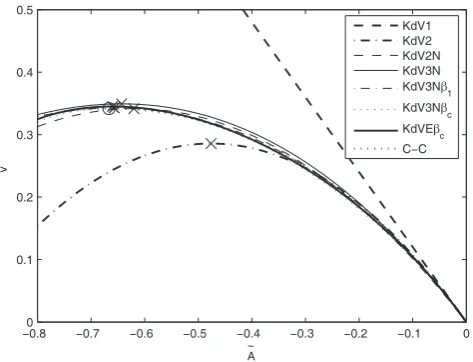
We consider several cases of the eigenvalue relation given in Eq. (34). First, we consider the case, termed KdVEβc,
with the exact nonlinear phase speed and the exact expres-sion forD˜E(Z)˜ . The variation of the eigenvalue (alt., the
solitary wave speed) with wave amplitude, as computed from Eq. (34), is presented in Fig. 6 for the particular depth ratio corresponding to=2/3. This exact result is compared in Fig. 6 with various alternate evolution models defined in the previous section. Analytic expressions for the eigenvalue for the different models are summarized in Appendix A. Fig. 6 shows that the eigenvalue for KdV1 provides a reasonable approximation for the speed of nonlinear wave features only for wave amplitudes| ˜ζ|<0.1. Further, KdV2 provides a use-ful approximation for wave amplitudes satisfying roughly
−0.8 −0.7 −0.6 −0.5 −0.4 −0.3 −0.2 −0.1 0 0
0.1 0.2 0.3 0.4 0.5
A
v
KdV1 KdV2 KdV2N KdV3N KdV3Nβ1 KdV3Nβc KdVEβc C−C
~
~
Fig. 6. Comparison of the dependence of the eigenvaluev˜on soli-tary wave amplitude for=2/3.
yield a maximum value for the eigenvalue (alt., solitary wave speed) at some intermediate amplitude. This point will be addressed further in a subsequent paragraph.
The next solution component of the various proposed evo-lution models that we compare is the profile of solitary waves. Profiles for specified amplitudes obtained using dif-ferent evolution models are shown in Fig. 7 for the particu-lar depth ratio given by=2/3. As expected, profile forms differ only marginally at low amplitudes, but significant dis-parities emerge as the amplitude increases. At low ampli-tudes the wave width diminishes with increasing amplitude for all models, a result that holds uniformly for KdV1, as is well known. However, as the amplitude increases (alt., as the degree of nonlinearity becomes increasingly signifi-cant), all models with the sole exception of KdV1 manifest a reversal in this trend of wave width increasing with wave amplitude. In particular, the profile obtained using KdV2 becomes quite wide with a flat trough when the amplitude is
˜
A=−0.47. This amplitude is just marginally below the limit-ing amplitudeA˜lim=− ˜µ1/µ˜2=−0.47619· · ·for KdV2. An analytical expression for this limiting amplitude is obtained in straightforward fashion from the functional relation for a solitary wave solution of KdV2
˜
Z(X)˜ = ˜A 1−T 2
1−bT2; T ≡tanh(K ˜ X);
b= − α˜2 ˜ A
2α˜1+ ˜α2A˜
. (35)
The limiting wave amplitude corresponds to that for which the parameterbapproaches the value of unity from below.
As evident in Fig. 7, wave profiles for KdV2N and KdV3N at an amplitude of A˜=−0.6 are nearly coincident, but the profile of the wave predicted by KdV1 is significantly more narrow. This characteristic under-prediction of the width
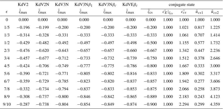
of the profile by KdV1 for higher wave amplitudes is well-known based on established results using KdV2 models (e.g., Evans and Ford, 1996; Lamb and Wan, 1998; Grimshaw, 2002; Holloway and Pelinovsky, 2002). However, the results presented here suggest that the widening of the wave profile is significantly over-estimated by KdV2. The widening effect beyond that corresponding to KdV1 becomes significant only at amplitudes in excess of the limiting value for KdV2. We point out for emphasis that the amplitudeζ˜1(i.e., the dimen-sionless wave amplitude based on the controlling dimension) for the particular case of=2/3 corresponding to the com-puted profiles shown in Fig. 7a isζ˜1=−1.5 whenζ˜=−0.5, and that the wave profile predicted by KdV1 is actually a “not-so-unreasonable” approximation when compared with the profile based on KdV3N at this large amplitude state. The profile shown in the last panel of Fig. 7a for an ampli-tude ofA˜=−0.64 does not include data for KdV2N because the amplitude exceeds the limiting value for this model. The widening effect for KdV3N relative to KdV1 at this ampli-tude is partially due to the fact that the ampliampli-tudeA˜=−0.64 is only slightly below the value ofA˜limfor KdV3N at=2/3. As discussed above, the models excluding KdV1 possess limiting amplitudes which, when approached from below, define conditions where the wave profile broadens signifi-cantly, even to the point where the profile approaches a front separating two uniform states. This naturally introduces the notion of conjugate states as introduced by Benjamin (1966), and computed by Turner and Vanden-Broeck (1988) and de-scribed in further detail by Amick and Turner (1986) and by Evans and Ford (1996). Values of the limiting solitary wave amplitudes for the models KdV2, KdV2N, KdV3N, KdV3Nβ1, KdV3Nβcand KdVEβcare presented in Table 2
for a range of depth ratios, and these limiting amplitudes are compared with results of the conjugate state amplitude computed using the theory of Amick and Turner (1986). For the special case of a two-layer stratification with a rigid up-per surface, the environmental case under examination here, Amick and Turner (1986) obtained an analytic solution for the conjugate state. When the Boussinesq approximation is invoked, and when their results are transposed in terms of the non-dimensional variables used herein, the conjugate state is defined simply by the relations
˜
ζcs = −; c˜2cs=
1 1−2; u˜
2
cs1= 1
˜ u2cs2
=1−
1+. (36)
(a)
(b)
A =−0.6 ε=2/3
A =−0.64 ε=2/3
A =−0.6 ε=4/5
A =−0.6 ε=7/8 ~
~ ~
~ −0.6
−0.4 −0.2 0
A =−0.1
ζ
~
−0.6 −0.4 −0.2 0
A =−0.2
−0.6 −0.4 −0.2 0
A =−0.4
ζ
~
−0.6 −0.4 −0.2 0
A =−0.47
−20 −10 0 10 20 −0.6
−0.4 −0.2 0
A =−0.6
ζ
~
X
−20 −10 0 10 20 −0.6
−0.4 −0.2 0
A =−0.64
X KdV1
KdV2 KdV2N KdV3N
~
~
~ ~
~
~
~ ~
−0.6 −0.4 −0.2 0
ζ
~
−0.6 −0.4 −0.2 0
ζ
~
−20 −10 0 10 20 X
~ −20 −10 0 10 20
X ~ −0.6
−0.4 −0.2 0
−0.6 −0.4 −0.2 0
−0.6 KdV3N KdV3Nβ1
KdV3Nβc
KdVEβc
Fig. 7. Comparison of solitary wave profile described by various evolution models at different amplitudes: (a) wave forms for=2/3 (left six panels); (b) wave forms for different values of(right four panels).
Included in Table 2 is a comparison of the speedc˜cs of
the “front” separating the conjugate states and the value of the speedc˜E(ζ˜cs)of the phase speed (Eq. 6) evaluated at the
amplitude of the conjugate state. These values are particu-larly disparate for low values of the depth ratio parameter, a difference that deserves some explanation. The computa-tion of the conjugate state is based on an integral theory that requires only an evaluation of the pressure at the upstream and downstream locations relative to the front. As such, it makes no approximation regarding the pressure distribution through the front, and accurately uses the appropriate hydro-static pressure distribution asymptotically far away from the front. On the other hand, the derivation of the phase speed given in Eq. (6) has explicitly used the leading order approx-imation for the pressure distribution in the limit of infinitely long waves everywhere through the wave profile, namely a hydrostatic distribution. This distinction naturally gives dis-parate values of the wave speed, and this different representa-tion of the pressure is especially apparent in the case of more nearly equal layer depths. When the layer depths are widely disparate, the front dynamics implicit in the conjugate state solution are more nearly hydrostatic.
We return now to the eigenvalue data exhibited in Fig. 6, and inject an observation regarding the existence of limit-ing amplitudes of stationary solutions (e.g., solitary waves) of the various evolution models. It was noted following Eq. (35) that the amplitude corresponding to the maximum of the eigenvalue for KdV2 and KdV2N coincided with the condition that the parameterb=1, the condition for Eq. (35)
−20 −10 0 10 20
−0.6 −0.4 −0.2 0
ζ
~
x ~
βc
C KdVE
C−
Fig. 8. Comparison of solitary wave profile described by KdVEβc and Choi-Camassa’s model for=2/3.
to describe an isolated front. In fact, our computations reveal that the limiting amplitude condition for all evolution mod-els corresponds to that amplitude for which the eigenvalue reaches a maximum. Of course, the eigenvalue for KdV1 has no local maximum and, therefore, KdV1 does not possess a limiting amplitude. For this reason, a mark denoting the peak of the eigenvalue is placed on the curves in Fig. 6, points that correspond to the limiting amplitudes for each of the models represented in the figure.
Table 2. Limiting wave amplitudes for different evolution models, and comparison with the theory of conjugate states.
KdV2 KdV2N KdV3N KdV3Nβ1 KdV3Nβc KdVEβc conjugate state
ζ˜max ζ˜max ζ˜max ζ˜max ζ˜max ζ˜max ζ˜cs c˜E|ζcs ccs˜ u˜cs1 u˜cs2
0 0.000 0.000 0.000 0.000 0.000 0.000 0.000 1.000 1.000 1.000 1.000
1/5 −0.196 −0.199 −0.200 −0.200 −0.200 −0.200 −0.200 1.000 1.021 0.817 1.225
1/3 −0.314 −0.328 −0.331 −0.333 −0.333 −0.333 −0.333 1.000 1.061 0.707 1.414
1/2 −0.429 −0.482 −0.492 −0.497 −0.497 −0.498 −0.500 1.000 1.155 0.577 1.732
2/3 −0.476 −0.620 −0.643 −0.657 −0.657 −0.660 −0.667 1.000 1.342 0.447 2.236
3/4 −0.457 −0.677 −0.712 −0.733 −0.732 −0.739 −0.750 1.000 1.512 0.378 2.646
4/5 −0.424 −0.706 −0.749 −0.777 −0.775 −0.786 −0.800 1.000 1.667 0.333 3.000
5/6 −0.390 −0.721 −0.771 −0.805 −0.802 −0.816 −0.833 1.000 1.809 0.302 3.317
6/7 −0.359 −0.729 −0.785 −0.823 −0.820 −0.837 −0.857 1.000 1.942 0.277 3.606
7/8 −0.332 −0.734 −0.794 −0.837 −0.833 −0.853 −0.875 1.000 2.066 0.258 3.873
8/9 −0.308 −0.737 −0.800 −0.846 −0.842 −0.865 −0.889 1.000 2.183 0.243 4.123
9/10 −0.287 −0.738 −0.804 −0.854 −0.849 −0.874 −0.900 1.000 2.294 0.299 4.359
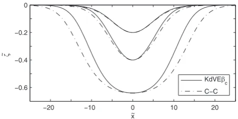
of the evolution models proposed here, the wave profiles for moderate amplitude waves of KdVEβc model are
com-pared with the corresponding Choi-Camassa (C-C) wave for
=2/3 in Fig. 8. It is seen that the KdVEβc profile slightly
underestimates the width of the wave profile, a consequence (we conjecture) of inadequacies of the approximate represen-tation of nonlinear dispersive effects in Eqs.(26) and (27). In regard to the speed and amplitudes of the limiting wave, the Choi-Camassa predictions are necessarily identical with the conjugate state values given in Table 2.
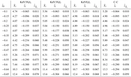
To compare the solitary wave profiles predicted by the var-ious evolution models at a further level of detail, we evaluate the spatial locationX˜i of the inflection point of the profile,
the wave amplitudeζ˜i at the inflection point, and the wave
slopeζ˜X˜
i at the inflection point. These data are presented in Table 3 for profiles computed using the depth ratio corre-sponding to=2/3.
Data do not appear in some columns because the selected amplitude in the leading column exceeds the limiting ampli-tude for the particular model. The wave width, as represented by the location of the inflection pointX˜
i, diminishes with
in-creasing wave amplitude in all models when the amplitude is small, but most emphatically for KdV1. In the models other than KdV1, the width begins to increase with increas-ing wave amplitude beyond modest amplitudes of the order
˜
ζ0≈−0.3. The increase in wave width becomes quite rapid as these profiles approach their limiting amplitudes.
The last column of Table 3 contains corresponding data obtained from Choi and Camassa’s exact, stationary solu-tion. One observes that KdV3Nβcmodel under estimates the
wave width by about 7% at an amplitude ofζ˜0=0.4, but the wave speeds are essentially identical. Hence, the KdV3Nβc
model, for example, provides a nonlinear evolution equation for moderately large waves in which the position, phase rela-tions and characteristics of individual wave profiles are rep-resented with quite high fidelity. For point of reference, the valueζ˜0=0.4 corresponds to a wave amplitudeζ˜1=−1.2 for =2/3 (h2=5h1).
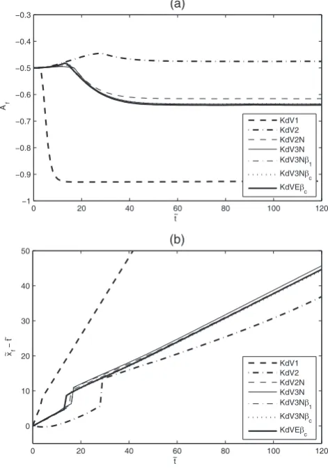
A third level of comparison of the different models is that of spatio-temporal evolution from a fixed initial condi-tion. For this purpose, an initial condition corresponding to a “non-equilibrium” form of a KdV2 solitary wave was cho-sen. That is, the profile defined by Eq. (35) was used, and the parameter set (A˜=−1/2 ,b=3/4,K=1/4) was purpose-fully selected in order to yield more than one leading solitary wave in the asymptotic state for KdV2 and the selected depth ratio=2/3. The result of a sequence of simulations on the semi-infinite line are shown in Fig. 9 where evolutionary data are shown for a fixed time in a spatial coordinate frame that moves with the linear, long-wave phase speedc0. A further comparison of the evolution leading to the wave forms shown in Fig. 9 is obtained by comparing the temporal variation of the amplitude of the leading wave in the packet, and its spa-tial position, as a function of time. These results are plotted in Fig. 10.
Table 3. Comparison of solitary wave inflection point data for different evolution models.
KdV1 KdV2 KdV2N KdV3N
˜
ζ0 X˜i ζ˜i ζ˜X˜
i
˜
Xi ζ˜i ζ˜X˜
i
˜
Xi ζ˜i ζ˜X˜
i
˜
Xi ζ˜i ζ˜X˜
i
−0.1 3.80 −0.067 0.013 4.32 −0.066 0.012 4.36 −0.066 0.012 4.31 −0.066 0.012
−0.15 3.10 −0.100 0.024 3.81 −0.098 0.021 3.77 −0.098 0.021 3.74 −0.098 0.021
−0.2 2.69 −0.133 0.038 3.62 −0.128 0.030 3.47 −0.130 0.031 3.46 −0.130 0.031
−0.25 2.40 −0.167 0.053 3.60 −0.158 0.040 3.32 −0.161 0.041 3.34 −0.160 0.041
−0.3 2.20 −0.200 0.069 3.76 −0.185 0.048 3.28 −0.191 0.051 3.31 −0.190 0.051
−0.35 2.03 −0.233 0.087 4.12 −0.208 0.055 3.33 −0.219 0.061 3.36 −0.218 0.061
−0.4 1.90 −0.267 0.107 4.87 −0.226 0.060 3.47 −0.245 0.070 3.51 −0.245 0.070
−0.45 1.79 −0.300 0.127 6.74 −0.237 0.063 3.73 −0.269 0.079 3.75 −0.268 0.077
−0.47 1.75 −0.313 0.136 9.42 −0.238 0.064 3.88 −0.277 0.081 3.89 −0.277 0.080
−0.5 1.70 −0.333 0.149 – – – 4.18 -0.288 0.084 4.16 −0.288 0.084
−0.55 1.62 −0.367 0.172 – – – 4.99 -0.302 0.088 4.83 −0.304 0.088
−0.6 1.55 −0.400 0.196 – – – 7.09 -0.309 0.090 6.16 −0.313 0.091
−0.64 1.50 −0.427 0.216 – – – – – – 10.8 −0.316 0.092
−0.65 1.49 −0.433 0.221 – – – – – – – – –
Table 3. Continued.
KdV3Nβ1 KdV3Nβc KdVEβc C-C
˜
ζ0 X˜i ζ˜i ζ˜X˜
i
˜
Xi ζ˜i ζ˜X˜
i
˜
Xi ζ˜i ζ˜X˜
i
˜
Xi ζ˜i ζ˜X˜
i
−0.1 4.74 −0.065 0.011 5.56 −0.063 0.010 5.33 −0.063 0.011 5.20 −0.064 0.010
−0.15 4.27 −0.096 0.020 5.19 −0.093 0.017 4.98 −0.093 0.018 4.90 −0.095 0.017
−0.2 4.07 −0.126 0.028 5.05 −0.122 0.024 4.88 −0.122 0.025 4.86 −0.124 0.024
−0.25 4.02 −0.155 0.037 5.04 −0.150 0.031 4.89 −0.150 0.032 4.96 −0.153 0.031
−0.3 4.07 −0.183 0.045 5.11 −0.177 0.038 4.98 −0.176 0.039 5.17 −0.179 0.037
−0.35 4.20 −0.209 0.053 5.26 −0.203 0.044 5.13 −0.202 0.045 5.48 −0.205 0.042
−0.4 4.42 −0.234 0.060 5.48 −0.228 0.050 5.36 −0.227 0.051 5.89 −0.228 0.047
−0.45 4.75 −0.256 0.066 5.82 −0.251 0.055 5.69 −0.249 0.056 6.45 −0.249 0.051
−0.47 4.93 −0.264 0.068 5.99 −0.259 0.057 5.86 −0.258 0.058 6.73 −0.256 0.052
−0.5 5.26 −0.275 0.071 6.31 −0.271 0.059 6.16 −0.270 0.061 7.22 −0.266 0.054
−0.55 6.04 −0.290 0.075 7.09 −0.287 0.062 6.89 −0.286 0.064 8.34 −0.280 0.057
−0.6 7.44 −0.300 0.077 8.50 −0.299 0.065 8.19 −0.298 0.067 10.2 −0.290 0.058
−0.64 10.3 −0.303 0.078 11.4 −0.303 0.065 10.7 −0.303 0.067 13.3 −0.294 0.059
−0.65 12.4 −0.304 0.078 13.6 −0.304 0.066 12.4 −0.304 0.068 14.9 −0.295 0.059
ζt+
1 2
∂c
∂xζ +c0c˜E( ˜
ζ )ζx+β0c0(β(˜ ζ )˜ c˜E(ζ )ζ˜ xx)x=0,(37)
In this equation we intend that evaluation of the rarefaction
−200 0 20 40 60 80 100 120 140 160 1
2 3 4 5 6 7 8 9
x − t
t = 0 KdV1 KdV2 KdV2N KdV3N KdV3Nβ1 KdV3Nβc KdVE
t = 100
0 10 20 30 40 50 60 70
0 1 2 3 4 5 6
x − t
KdV2 KdV2N KdV3N KdV3Nβ1 KdV3Nβc KdVE
t = 120
~ ~
~
~
~ ~
~
Fig. 9. Comparison of spatial wave forms at a fixed time as derived from various models using the same initial condition (=2/3).
and ignoring the implicit dependence through the amplitude functionζ (x, t )˜ . In this case, for example, the rarefaction term for the generalized equation (Eq. 26) becomes
1 2
∂c ∂x =
1 2
˜ cE(ζ , )˜
dc0 dx +c0
∂c˜E ∂
d dx
. (38)
In order to exhibit the effect of nonlinearity entering via this term, the initial value problem was solved using a depth variation where varied gradually (i.e., over a distance of roughly 200(=2H ) upper-layer depths) from its initial (upstream) value of1=3/4 to its shelf (downstream) value 2=1/3 according to the relation
0 20 40 60 80 100 120
−1 −0.9 −0.8 −0.7 −0.6 −0.5 −0.4 −0.3
t Af
(a)
0 20 40 60 80 100 120
0 10 20 30 40 50
t xf
− t
(b)
KdV1 KdV2 KdV2N KdV3N KdV3Nβ1 KdV3Nβc KdVEβc KdV1 KdV2 KdV2N KdV3N KdV3Nβ1 KdV3Nβc KdVEβc
~
~
~ ~
~
Fig. 10. Change in (a) leading wave front amplitudeA˜f and (b) its position (x˜f− ˜t) as a function of time (=2/3).
(x)˜ = 1+2
2 −
1−2 2 tanh
x˜
H
. (39)
The initial condition in this simulation was the same as that used for the simulations presented in Fig. 9. Simulations were performed for both the weakly-nonlinear version KdV2 and for the strongly nonlinear version KdV2N. Waveforms obtained at several times are compared in Fig. 11. As ex-pected, the KdV2N waveform travels faster, and has a nar-rower leading solitary wave since the limiting amplitude for KdV2 is smaller, resulting in a more extended and flattened trough. The waveforms appearing at a late time on the shelf are shown in Fig. 12.
−600 −400 −200 0 200 400 600 0
1 2 3 4 5
x
t=0 t=200 t=200 t=400 t=400 t=600 t=600 t=1000 t=1000
KdV2 KdV2N KdV2 KdV2N KdV2 KdV2N KdV2 KdV2N
topography (not to scale)
~
~ ~ ~
~
~
~
~
~
~
Fig. 11. Comparison of shoaling wave forms for KdV2 and KdV2N for evolution from a common initial condition.
KdV2N waveform, and has a remnant form even att˜=1800. We speculate that the formation of this pair-like form occurs when the lead wave with near-limiting amplitude undergoes deformation while passing over the topographic variation. The individual entities in this pair-like form have (nearly) identical amplitudes and propagate with (nearly) fixed prox-imity to each other.
5 Concluding remarks
Several models have been proposed for the evolution of lowest-mode, internal wave disturbances based on the ex-act relation for the phase speed for nonlinear wave propa-gation along a single characteristic in the long wave (hydro-static) limit. The proposed models have been examined for the purpose of providing a reliable, quantitative description of the evolutionary character of waves in a two-layer strati-fication with arbitrary amplitude. The need for models valid for strongly nonlinear evolution is readily seen when consid-ering several documented cases. For example, waveforms with amplitudes (ζ˜
1≈−0.8, ζ˜≈−0.32) in an environment with =0.59 have been reported by Pingree and Mardell (1985); waveforms with (ζ˜1≈−2.1,ζ˜≈−0.32) in an environ-ment with=0.85 have been reported by Trevorrow (1998); and waveforms with (ζ˜1=−4, ζ˜=−0.4) in an environment with=0.91 have been reported by Stanton and Ostrovsky (1998). In weakly nonlinear theory the asymptotic expan-sion presupposes that the characteristic amplitude parameter
10000 1050 1100 1150 1200 1250 1300 1350 0.1
0.2 0.3 0.4 0.5
x
KdV2 KdV2N
~
Fig. 12. Comparison of shoaling wave forms for KdV2 and KdV2N att˜=1800.
| ˜ζ1|1. In light of these observations, the need for reliable models for strongly nonlinear evolution is indeed obvious.
Table 4. Properties of solitary waves of KdVEβcfor environments having deep lower layers.
=4/5 =7/8 =9/10
˜
ζ0 X˜i ζ˜i ζ˜X˜
i
˜
Xi ζ˜i ζ˜X˜
i
˜
Xi ζ˜i ζ˜X˜
i
−0.1 4.59 −0.062 0.013 4.34 −0.059 0.015 4.33 −0.058 0.015
−0.2 4.49 −0.117 0.029 4.56 −0.111 0.031 4.69 −0.108 0.031
−0.3 4.70 −0.168 0.044 4.93 −0.159 0.045 5.15 −0.155 0.045
−0.4 5.03 −0.217 0.057 5.34 −0.205 0.058 5.62 −0.199 0.057
−0.5 5.49 −0.262 0.069 5.81 −0.248 0.069 6.12 −0.241 0.068
−0.6 6.22 −0.302 0.078 6.42 −0.288 0.078 6.74 −0.280 0.077
−0.7 7.68 −0.330 0.084 7.36 −0.322 0.085 7.62 −0.314 0.083
−0.8 – – – 9.53 -0.343 0.090 9.39 −0.338 0.088
for a continuously stratified thermoclinic layer of finite thick-ness, and then provide suggested values of the layer depths to be used in an equivalent two-layer model.
Examination of Figs. 3 and 4 suggests that KdV2 would considerably underestimate the nonlinearity for all cases listed above. By contrast, the KdV2N evolutionary model could be expected to yield a respectably satisfactory degree of correspondence between model results and the level of
| ˜ζ|values associated with these observations. However, for cases where amplitudes are such that| ˜ζ|>0.5−0.6, KdV3N will be required to realize a reasonable fidelity between model results and measured data. Advantages of KdV2N include analytical expressions for both the form of a soli-tary wave and its eigenspeed, the same advantages associ-ated with KdV1 and KdV2. Hence, wave properties can be readily computed and compared with laboratory or field data, and simple scaling laws for these waves are available. Fur-thermore, KdV2N provides a quite respectable approxima-tion for the limiting amplitude, particularly in comparison to KdV2, as seen in Table 2. Of course, an analytical expression for solitary wave solutions of KdV3N is certainly expected to be accessible as well, although preliminary efforts on our part have not yet yielded success in this venture. Hence, the argument in favor of KdV2N over KdV3N on the basis of possessing a solitary wave solution, with its specific scaling relationships, is not entirely compelling.
Comparing data for solitary wave profiles for KdV2N and KdV3N contained in Table 3, it is clear that the difference between the indicated values of the width of the wave pro-file only becomes significant as the limiting amplitude is ap-proached. On the other hand, comparison of profile widths for KdV3N with those for KdV3Nβ1 and KdV3Nβc, it is
seen that nonlinear dispersive effects serve to increase the wave width significantly, with the exception being when wave amplitudes are near their limiting value for a specific model. With this effect of nonlinear dispersion in view, it is worth noting that, although no data have been included
herein, one could readily compute corresponding properties for such cases as KdV2Nβ1 and KdV2Nβc. Furthermore,
since physical environments with relatively deep lower lay-ers (i.e., values ofapproaching unity) are not uncommon, data pertaining to KdVEβc for several depth ratios are
pre-sented in Table 4.
Appendix A
The eigenvalue relation for case KdV3Nβcis, after carrying
through the evaluation of the integral terms in Eq. (34),
˜
v= ˜V −1= − 1 JV
˜
µ1 2 Jµ1+
˜ µ2
3 Jµ2+
˜ µ3
4 Jµ3
.
The variousJkterms in this relation are defined as JV = −
dm
2
(1−P )ln 1+S
1−P
+(1+P )ln 1−
S
1+P
;
Jµ1 = −d
2
m(P +S)+ dm2
2
(1−P )2ln 1+S
1−P
−(1+P )2ln 1−S
1+P
;
Jµ2 = −
dm3
2 n
(S2−P2)+6dm(S+P ) +(1−P )3ln
1+S 1−P
+(1+P )3ln 1−S
1+P
;
Jµ3 = −d
4
m
n
(1+6dm2)(P+S)+2dm(S2−P2) +1
3(P 3+S3)
+d 4
m
2
(1−P )4ln 1+S
1−P
−(1+P )4ln 1−S
1+P
In writing these expressions we have employed the definition
P = ˜ ζDm
dm
; S= ˜ ζ − ˜ζDm
dm .
In a corresponding manner, the relevant Jk terms for
KdV3Nβ1are, upon using the definitionS1= ˜ζ1+, JV = −
1 2
(1−)ln 1+S
1 1+
+(1+)ln 1−S
1 1−
;
Jµ1 = − ˜ζ +
1 2
(1+)2ln 1+S
1 1+
−(1−)2
1−S 1
1−
;
Jµ2 =3ζ˜−
1 2(S
2 1−
2)−1 2
(1+)3ln 1+S
1
1+
+(1−)3ln 1−
S1 1−
;
Jµ3 = −(1+6
2)ζ˜+2(S2 1−
2)
−1
3(S 3 1−
3)+1 2
(1+)4ln 1+S
1
1+
−(1−)4ln 1−
S1 1−
.
Appendix B
We present calculations aimed at guiding the formation of an equivalent two-layer model to characterize long wave prop-agation in a wave guide which contains a thermoclinic layer of finite thickness. For this purpose we consider an environ-mental model where a single thermoclinic layer with con-stant Brunt-V¨ais¨al¨a frequency having thicknesshm is
posi-tioned in a wave guide such that the distance from the upper surface to the mid-depth of the stratified layer ish10. The total depth of the wave guide ish10+h20,h20being the dis-tance from the middle of the thermocline to the bottom of the wave guide. The goal is to specify the equivalent upper-layer (mixed layer) depthhequiv=h1in a two-layer environmental model with total fluid depthh1+h2=h10+h20 for different thicknesseshmof the thermoclinic layer.
Several different criteria for defining an equivalent two-layer model can be proposed. To establish conditions for an equivalent model, the value of the reduced grav-ity g=g(ρ˜ 1−ρ2)/ρ1 must be specified. We take ρ1 and ρ2 to be the epilimnion and hypolimnion densities in the continuously-stratified environment. Thus, within the Boussinesq approximation, the value ofg˜is equal to the in-tegral of the Brunt-V¨ais¨al¨a frequency across the depthhmof
the stratified layer. Withg˜fixed, one further condition must be prescribed to fix the remaining free parameter – the equiv-alent upper-layer depthhequiv(equal toh1in the text of this
−1 −0.8 −0.6 −0.4 −0.2 0
0.6 0.7 0.8 0.9 1 1.1
A/h
10
hequiv
/h10 hm/h10
0.6 h
10/h20=1/3 (ε=1/2)
h
10/h20=1/5 (ε=2/3)
0.4 = 0.2
Fig. B1. Equivalent upper layer depth based on matching phase speed of solitary wave as a function of wave amplitude.
paper). We present calculations here based on two different options for this purpose, and then compare the consequent values of hequiv. First, we constrain the speed of lowest-mode, isolated (solitary) wave features in the continuously-stratified case to correspond with those in an equivalent two-layer model. This criterion forces a correspondence between the location of waves relative to their source, and also phase relationships between different waves in a packet. Second, we choose to match the peak isopycnal displacement (wave amplitude) in the continuously-stratified model with the in-terface displacement in the equivalent two-layer model.
It is immediately clear that each of these bases for equiva-lence depend on the wave amplitude. In order to establish equivalence, therefore, it seems that comparable approxi-mations for nonlinear and dispersive effects should be em-ployed for each environmental model. However, since a fully-nonlinear representation of the nonlinear phase speed comparable to Eq. (6) is not available for the continuously-stratified case, we choose to use the KdV2 description of wave evolution for both environments. For the two-layer model we employ the relations given by Eqs. (1–5) in the text, and for the continuously-stratified wave-guide we use the KdV2 description as presented by Grimshaw (2002).
−1 −0.8 −0.6 −0.4 −0.2 0 0.9
1 1.1 1.2
A/h 10 hequiv
/h10
h
m/h10=0.2
h
10/h20=1/3 (ε=1/2)
h
10/h20=1/5 (ε=2/3)
0.4 0.6
Fig. B2. Equivalent upper layer depth based on matching peak isopycnal displacement as a function of wave amplitude.
the reduction in equivalent upper-layer depth increases as the thicknesshm of the thermoclinic layer increases. Further,
the variation ofhequivwith wave amplitude is much weaker when the layer depths are less disparate. In fact, in the deeper case withh10/ h20=1/5, the results show that thehequiv>h10 when the wave amplitude becomes large (i.e., larger nega-tive values). Of course, if the results shown in Fig. 3 for the two-layer model are also indicative of corresponding results for the continuously-stratified case, the utility of the KdV2 approximation should properly be restricted to amplitudes
˜
A=|A/ h|<0.3.
Figure B2 presents results for the equivalent two-layer depth hequiv based on the alternate criterion of matching the peak isopycnal displacement. To realize correspond-ing isopycnal displacements, the value ofhequivis found, in contrast to results shown in Fig. B1, to be greater than the mid-thermocline depthh10. Furthermore, the value ofhequiv based on this criterion exhibits quite sensitive amplitude de-pendence, withhequivdecreasing toward the mid-thermocline depth as the wave amplitude increases.
This brief consideration of issues underlying the selection of an equivalent two-layer model shows clearly that some physical effects must be compromised in the use of a sim-plified environmental model. In this connection, we prefer to base the equivalent model on the first criterion. That is, we prefer that wave arrival times and phase information be replicated as accurately as possible. Employing this criterion, values of hequiv have been computed for several choices of the parameters eps andhm/ h10. The computed values of hequiv, having the form shown in Fig. B1, were then averaged over that range of wave amplitudes satisfying the condition 0.9≤|cKdV2/cE|≤1.0 for the two-layer model.
Results of this calculation are summarized in Table B1. We suggest that the values ofhequivpresented in Table B1 should
Table B1. Equivalent upper layer depth for different thickness of thermoclinic layer.
hm/ h10
h10/ h20 0.2 0.4 0.6 0.8 1.0
1/3 1/2 0.88 0.79 0.71 0.63 0.56
1/5 2/3 0.93 0.86 0.79 0.72 0.66
1/7 3/4 0.94 0.88 0.81 0.75 0.69
1/9 4/5 0.94 0.88 0.82 0.76 0.70
1/11 5/6 0.94 0.89 0.83 0.77 0.71
1/13 6/7 0.94 0.89 0.83 0.77 0.72
provide a useful guide for defining quantitatively equivalent two-layer models for natural environments containing single, prominent thermocline having finite thickness.
Edited by: A. Osborne Reviewed by: two referees
References
Amick, C. and Turner, R.: A global theory of internal waves in two-fluid systems., Trans. Am. Math. Soc., 298, 431–481, 1986. Antenucci, J., Imberger, J., and Saggio, A.: Seasonal evolution of
the basin-scale internal wave field in a large stratified lake., Lim-nol. Oceanogr., 45, 1621–1638, 2000.
Apel, J., Holbrook, J., Liu, A., and Tsai, J.: The Sulu Sea internal soliton experiment., J. Phys. Oceanogr., 15, 1625–1651, 1985. Benjamin, T.: Internal waves of finite amplitude and permanent
form., J. Fluid Mech., 25, 241–270, 1966.
Bogucki, D. and Redekopp, L.: A mechanism for sediment re-suspension by internal solitary waves., Geophys. Res. Lett., 26, 1317–1320, 1999.
Bogucki, D., Dickey, T., and Redekopp, L.: Sediment resuspension and mixing by resonantly generated internal solitary waves., J. Phys. Oceanogr., 27, 1181–1196, 1997.
Bogucki, D., Redekopp, L., and Barth, J.: Internal solitary waves in the Coastal Mixing and Optics 1996 experiment: Multimodal structure and resuspension, J. Geophys. Res., 110, C02024, doi:10.1029/2003JC002253, 2005.
Choi, W. and Camassa, R.: Fully nonlinear internal waves in a two-fluid system., J. Fluid Mech., 396, 1–36, 1999.
Djordjevic, V. and Redekopp, L.: The fission and disintegration of internal solitary waves moving over two-dimensional topogra-phy., J. Phys. Oceanogr., 8, 1016–1024, 1978.
Duda, T., Lynch, J., Irish, J., Reardsley, R., Ramp, S., Chui, C., Tang, T., and Yang, Y.: Internal tide and nonlinear internal wave behavior at the continental slope in the northern South China Sea., IEEE J. Oceanic Eng., 29, 1105–1130, 2004.
Evans, W. and Ford, M.: An integral equation approach to internal (2-layer) solitary waves., Phys. Fluids, 8, 2032–2047, 1996. Grimshaw, R.: Internal solitary waves, chap. 1, pp. 1–27, Kluwer
Helfrich, K. and Melville, W.: Long nonlinear internal waves., Annu. Rev. Fluid Mech., 38, 395–425, 2006.
Holloway, P. and Pelinovsky, E.: Internal solitary waves, chap. 2, pp. 29–60, Kluwer Academic, Boston, 2002.
Lamb, K. and Wan, B.: Conjugate flows and flat solitary waves for a continuously stratified fluid., Phys. Fluids, 10, 2061–2079, 1998. Osborne, A. and Burch, T.: Internal solitons in the Andaman Sea.,
Science, 208, 451–460, 1980.
Ostrovsky, L. and Grue, J.: Evolution equations for strongly non-linear internal waves., Phys. Fluids, 15, 2934–2948, 2003. Ostrovsky, L. and Stepanyants, Y. A.: Do internal solitons exist in
the ocean?, Rev. Geophys., 27, 293–310, 1989.
Ostrovsky, L. and Stepanyants, Y. A.: Internal solitons in laboratory experiments: Comparison with theoretical models, Chaos, 15, 037 111, doi:10.1063/1.2107087, 2005.
Pingree, R. and Mardell, G.: Solitary internal waves in the Celtic Sea., Prog. Oceanogr., 14, 431–441, 1985.
Scotti, A. and Pineda, J.: Observation of very large and steep inter-nal waves of elevation near the Massachusssetts coast., Geophys. Res. Lett., 31, L22 307, doi:1029/2004GL021052, 2004.
Slunyaev, A., Pelinovsky, E., Poloukhina, O., and Gavrilyuk, S.: The Gardner equation as the model for long internal waves., in: Topical Problems of Nonlinear Wave Physics, Proc. Int’l. Symp., pp. 368–369, Inst. of Appl. Phys., RAS, Nizhny Novgorod, 2003. Stanton, T. and Ostrovsky, L.: Observations of highly nonlinear in-ternal solitons over the continental shelf., Geophys. Res. Lett., 25, 2695–2698, doi:10.1029/98GL01772, 1998.
Stastna, M. and Lamb, K.: Vortex shedding and sediment resuspen-tion associated with the interacresuspen-tion of an internal solitary wave and the bottom boundary layer., Geophys. Res. Lett., 29(11), 1512, doi:10.1029/2001GL014070, 2002.
Trevorrow, M.: Observations of internal solitary waves near the Oregon coast with an inverted echo sounder., J. Geophys. Res. – Oceans, 1041, 7671–7680, 1998.