www.atmos-meas-tech.net/5/2723/2012/ doi:10.5194/amt-5-2723-2012
© Author(s) 2012. CC Attribution 3.0 License.
Measurement
Techniques
Development of a new data-processing method for SKYNET sky
radiometer observations
M. Hashimoto1, T. Nakajima1, O. Dubovik2, M. Campanelli3, H. Che4, P. Khatri5, T. Takamura5, and G. Pandithurai6
1Atmosphere and Ocean Research Institute (AORI), University of Tokyo, 5-1-5 Kashiwanoha, Kashiwa, Chiba 277-8568, Japan
2Laboratoire d’Optique Atmosph´erique, UMR8518, CNRS – Universit´e de Lille 1, Villeneuve d’Ascq, France 3Institute of Atmospheric Sciences and Climate, Italian National Research Council, Via Fosso del Cavaliere, Roma Tor Vergata, Italy
4Key Laboratory of Atmospheric Chemistry (LAC), Centre for Atmosphere Watch and Services (CAWAS), Chinese Academy of Meteorological Sciences (CAMS), CMA, Beijing 100081, China
5Center for Environmental Remote Sensing, Chiba University, 1-33 Yayoi-cho, Chiba 263-8522, Japan 6Centre for Climate Change Research, Indian Institute of Tropical Meteorology, 411 008 Pune, India
Correspondence to: T. Nakajima ([email protected])
Received: 23 March 2012 – Published in Atmos. Meas. Tech. Discuss.: 25 June 2012 Revised: 14 October 2012 – Accepted: 23 October 2012 – Published: 15 November 2012
Abstract. In order to reduce uncertainty in the estimation of
Direct Aerosol Radiative Forcing (DARF), it is important to improve the estimation of the single scattering albedo (SSA). In this study, we propose a new data processing method to improve SSA retrievals for the SKYNET sky radiometer net-work, which is one of the growing number of networks of sun-sky photometers, such as NASA AERONET and others. There are several reports that SSA values from SKYNET have a bias compared to those from AERONET, which is regarded to be the most accurate due to its rigorous cali-bration routines and data quality and cloud screening algo-rithms. We investigated possible causes of errors in SSA that might explain the known biases through sensitivity experi-ments using a numerical model, and also using real data at the SKYNET sites at Pune (18.616◦N/73.800◦E) in India and Beijing (39.586◦N/116.229◦E) in China. Sensitivity ex-periments showed that an uncertainty of the order of±0.03 in the SSA value can be caused by a possible error in the ground surface albedo or solid view angle assumed for each observation site. Another candidate for possible error in the SSA was found in cirrus contamination generated by imper-fect cloud screening in the SKYNET data processing. There-fore, we developed a new data quality control method to get rid of low quality or cloud contamination data, and we ap-plied this method to the real observation data at the Pune site
in SKYNET. After applying this method to the observation data, we were able to screen out a large amount of cirrus-contaminated data and to reduce the deviation in the SSA value from that of AERONET. We then estimated DARF us-ing data screened by our new method. The result showed that the method significantly reduced the difference of 5 W m−2 that existed between the SKYNET and AERONET values of DARF before screening. The present study also suggests the necessity of preparing suitable a priori information on the distribution of coarse particles ranging in radius between 10 µm and 30 µm for the analysis of heavily dust-laden atmo-spheric cases.
1 Introduction
have been conducted to reduce the uncertainties. Among these, ground-based measurement networks of scanning sun-sky multi-wavelength photometers, e.g., NASA AERONET (Holben et al., 1998), can measure and retrieve aerosol opti-cal properties that afford a key to accurately evaluating Direct Aerosol Radiative Forcing (DARF). In particular, the reliable retrieval of the single scattering albedo (SSA) of aerosols (e.g., Dubovik et al., 2002) is a unique function of these net-works. In this regard, it is important to recognize that accu-rate retrieval of the SSA is more difficult than estimation of the value of aerosol optical thickness (AOT) and size distri-bution (e.g., Loeb and Su, 2010; McComiskey et al., 2008). We refer to the normal optical thickness as optical thickness for normal incidence (Chandrasekhar, 1960). Continued ef-fort toward improving and validating SSA retrieval from net-works is, therefore, an important task for us to increase the accuracy of modeling aerosol climate effects.
SKYNET (Nakajima et al., 2007), the focus of our study, is a ground-based network of scanning sun-sky photometers called sky radiometers (Prede Co., Ltd, Tokyo, Japan) with observation sites spread over Asia and other areas. Direct and diffuse solar irradiances are measured with the sky radiome-ters, and are analyzed to derive the aerosol optical properties, such as AOT, SSA, complex refractive index, and volume size distribution function (SDF) by using SKYRAD.pack, a software package to analyze the sky radiometer data (Naka-jima et al., 1996). Aerosol optical properties retrieved from SKYNET have been used to investigate regional and sea-sonal characteristics of aerosols for climate and environmen-tal studies and to validate satellite remote sensing results (e.g., Higurashi and Nakajima, 2002; Kim et al., 2005; Sohn et al., 2007; Pandithurai et al., 2009; Campanelli et al., 2010; Khatri et al., 2010; Takenaka et al., 2011).
There are several reports that the AOT is obtained with high accuracy compared with that of the standard Langley method and with those from AERONET (Campanelli et al., 2007; Che et al., 2008). However, it is pointed out that the SSA values from SKYNET are 3 % to 8 % larger than those of AERONET at the Beijing site, although the retrieved AOT values from SKYNET agree with those from AERONET within about 1 % (Che et al., 2008). There are several aerosol types with SSA value close to 1. It is, however, claimed that the SKYNET SSA sometimes becomes unnaturally close to unity, as found at the Phimai site in Thailand (H. Tsuruta, personal communication, 2011) and at the Hyderabad site in India (Badarinath et al., 2011).
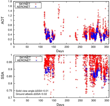
Figure 1 compares the values of AOT and SSA for SKYNET, at a wavelength of 0.5 µm, and for AERONET, at a wavelength of 0.5 µm, which are interpolated by a polyno-mial fit in logarithmic space with wavelength, at Pune from April through December 2008. The figure shows that the SKYNET AOT values are in close agreement with those of AERONET, whereas the SSA values from SKYNET varied widely, with a tendency to become larger than those from AERONET. Additionally, some SSA data are unnaturally
0 0.2 0.4 0.6 0.8 1 1.2 1.4 1.6 1.8
0 50 100 150 200 250 300 350
Aerosol Optical Thickness
Date number of 2008 Pune AOT(500nm) 2008/04/29-2008/12/31
SKYNET AERONET
0.7 0.75 0.8 0.85 0.9 0.95 1
0 50 100 150 200 250 300 350
Single Scattering Albedo
Date number of 2008 Pune SSA(500nm) 2008/04/29-2008/12/31
SKYNET AERONET
SSA
AOT
Days!!
Days!!
Solid view angle !SSA~0.01
Ground albedo !SSA~0.02
Fig. 1. Time series of AOT and SSA at a wavelength of 0.5 µm at
the Pune site. The upper and lower panels show AOT and SSA, respectively. The period is from April through December 2008. The horizontal axis is the time of Julian day from 1 January 2008. Daggers and crosses indicate the results of SKYNET retrieved by SKYRAD.pack version 4 and the results of AERONET, respec-tively.
close to unity, as reported in previous studies. It is difficult to explain this difference by the difference in wavelengths.
It should be noted that the working instruments located at the observation sites, operational systems, and analysis algorithms are somewhat different between two networks. AERONET Cimel sun/sky radiometer scans the sky at both sides of the sun to check the symmetry of spectral radiances relative to the sun in the almucantar by the AERONET pro-cessing criteria. The criteria are based on the assumption that the aerosols are uniformly distributed over the ground, and is helpful for the screening of cloud contamination data. On the other hand, the SKYNET Prede sky radiometer scans just one side in all the azimuths. For the cloud screening of AOT, AERONET and SKYNET adopt Smirnov et al. (2000) and Khatri and Takamura (2009), respectively. We describe the SKYNET cloud screening in Sect. 3.2.
sky radiance are carried out at each site by use of an improved version of the Langley plot method, and the solar disk scan-ning method for obtaiscan-ning calibration constants and solid view angles, respectively. Furthermore, the inversion calcu-lation methods adopted by these two networks are differ-ent. SKYNET adopts Phillips-Twomey method (Nakajima et al., 1996), while AERONET adopts the maximum likelihood method (MLM) combined with Phillips-Twomey method as a smoothing constraint (Dubovik and King, 2000). The AERONET algorithm includes the particle non-sphericity, but the SKYNET one does not in the present version. For the inversion method, we refer to it in Sect. 2.3.
To develop the technique to derive more accurate aerosol properties in the atmosphere, it is important to estimate the error included in the retrieval values and processes. The pur-pose of this study is to perform sensitivity studies of various aspects of the present SKYNET algorithms, though the true validation of the algorithm should be done through compar-ison with in situ measurements, which should be our next task. In this study, therefore, we investigated possible causes of error in the SSA retrieved from SKYNET through numer-ical experiments using a radiation transfer code and through data analysis with real observation data. On the basis of the results of the investigation, we suggest an improved method to estimate SSA more accurately. In Sect. 4, we evaluate DARF using improved aerosol optical parameters from the Pune and Beijing sites.
2 Numerical tests
This section describes sensitivity tests to investigate possible causes of error in SSA values from SKYNET.
2.1 SKYRAD.pack
SKYRAD.pack is an open source software package released on the OpenCLASTR web page (http://www.ccsr.u-tokyo.ac. jp/∼clastr/) for data analysis of direct and diffuse solar
radi-ation measurements to give the AOT, SSA, complex refrac-tive index, volume size distribution function (SDF), phase function, and so on. The present version of SKYRAD.pack (version 4) is used for operational analysis by the SKYNET data center at Chiba University (http://atmos.cr.chiba-u.ac. jp/) and the European Skynet Radiometers network (ESR, http://www.euroskyrad.net/index.html).
SKYRAD.pack utilizes monochromatic direct solar irradi-ance in W m−2µm−1,F, and relative diffuse solar radiance (sky radiance),R(2), defined by Eqs. (1) and (2) (Nakajima et al., 1996).
F =F0exp(−m0τ ) , (1)
R(2)= E(2)
F m01
=ωτ P (2)+q(2) , (2)
whereF0is extraterrestrial solar irradiance in W m−2µm−1, which is determined by the improved Langley method; E(2), the monochromatic sky irradiance in W m−2µm−1 measured at a scattering angle 2; τ,ω, and P (2)are the total optical thickness, SSA, and scattering phase function at scattering angle2for the column atmospheric air mass, respectively;m0is the optical air mass;1, the solid view angle (SVA) of the sky radiometer; andq(2), the contribu-tion of multiple scattering.
In the actual analysis, the measured values,F andE(2), are voltage outputs, andF0is a parameter to be determined by the improved Langley method in the voltage unit, called a calibration constant.1 is determined by the solar disk scanning method.
Equations (1) and (2) include information on the aerosol microphysical parameters along with molecular scattering, such as vertically integrated aerosol SDF,v(r), as a function of particle radius,r, and complex refractive index,m˜, as a function of wavelength,λ. The AOT,τa, and effective SSA, ωa, of aerosols in the atmospheric column can be derived from the following relations:
τa=
Z Ke
2 π r λ ,m˜
v (r)d lnr, (3a)
ωaτaPa(2)=
Z K
2,2π r
λ ,m˜
ν (r)d lnr, (3b)
v (r)= dV
d lnr = 4π
3 r 4dN
dr , (3c)
whereKeandK are kernel functions of the Fredholm inte-gral equations as a function of size parameterx(=2π/λand the complex refractive index. To solve Eqs. (1) through (3) as an inversion problem, these equations are formulated into a matrix formula by discretization of λ,2, and ln(r), and by weighting to make the solution stabilized as proposed by Nakajima et al. (1983):
f=Kx, (4)
wheref is an observation vector; K=K(m(λ))˜ , a matrix of kernel coefficients calculated for fixed values of complex re-fractive indexm(λ)˜ ; andx, a state vector containing values of size distributionvi=v (ri)withri equidistant on a loga-rithmic scale, i.e., ln(ri+1)−ln(ri)=const.
SKYRAD.pack uses two methods for removing the multi-ple scattering contribution in Eq. (2) and inversion of Eq. (4). The present inversion program, called version 4, uses the it-erative relaxation method of Nakajima et al. (1983, 1996) and a statistical regularization method (Turchin and Nozik, 1969) to derive an optimal solution by minimizing the fol-lowing cost function as proposed by Phillips (1962) and Twomey (1963):
where B is the second order derivative matrix with respect to the particle size in ln(r), to generate a priori informa-tion that force the obtained soluinforma-tionx to be a smooth func-tion of ln(r). The constant γ is a Lagrange multiplier co-efficient and is chosen so as to minimize the first term of the right-hand side of Eq. (5). The solution of Eq. (4) pro-vides smooth retrieval of size distributionv (r) correspond-ing to the minimum ofe2 defined by Eq. (5). However, in such an approach, both the solutionv (r)ande2depend on the assumed value of the complex refractive index m(λ)˜ , i.e.,e2=e2(m)˜ Correspondingly, if the value ofm(λ)˜ is un-known, the minimization of Eq. (5) can be performed for a set of different valuesm˜k(λ) (k=1,2, . . . , Nk), andm˜k(λ) corresponding to the smallest e2(m)˜ can be considered as a retrieved value of the complex refractive index. The dis-advantage of such a retrieval approach is that the retrieved
˜
mk(λ)can only be chosen from the predefined set of values
˜
mk(λ)(k=1,2, ..., Nk).
If the values of complex refractive indexm(λ˜ j)are di-rectly included in the state vector x, the discretized sys-tem analogous to Eq. (4) becomes non-linear and should be solved by non-linear iterative techniques. In addition, in order to ensure uniqueness of solution, the minimized cost function of Eq. (5) should be modified so that it includes constraints on the retrieved complex refractive index. This can be achieved, for example, by using the maximum like-lihood method (MLM) as defined by Rodgers (2000). This method is employed by version 5 and will be described in more detail in the next section.
2.2 Sensitivity tests for parameters for data processing
To investigate possible causes of error in the SSA retrieved from SKYNET, we analyzed simulated direct solar irradi-ances and sky radiirradi-ances using SKYRAD.pack.
Candidates for possible causes of error are as follows: (1) errors in the input geophysical parameters, such as ground surface albedo and initial condition values of complex re-fractive index; (2) instrumentation errors, such as minimum observable scattering angle and stray light, and calibration constants and solid view angles of the radiometer; (3) errors caused by inversion algorithms (type of inversion algorithm); and (4) errors attributed to the condition of the atmosphere, such as homogeneity in space and time and the total amount of aerosols in the atmosphere, that is, the value of AOT. The concept and methodology of the tests are somewhat consis-tent with earlier sensitivity studies conducted by Dubovik et al. (2000) for evaluating the accuracy of AERONET re-trievals.
We simulated observation data by using the Open-CLASTR software package for radiative transfer code called Rstar-6b (Radiance System for Transfer of Atmospheric Ra-diation version 6b) using the formulae of Nakajima and Tanaka (1986, 1988). We used the AFGL US standard for atmospheric conditions and the rural aerosol model
incorporated in Rstar-6b, which is based on the rural model of the WCP report (Deepak and Gerber, 1983). We set the solar zenith angleθ0=60◦and AOT = 0.5 for a wavelength of 0.5 µm. The ground surface albedo Ag, calibration con-stantF0, and SVA1are given as 0.2, 1, and 2.5×10⁻⁴str, respectively, at wavelengths of 0.4, 0.5, 0.675, 0.84, and 1.02 µm. In the analysis, we assumed an error of±5 % for F0,±5 % for SVA,±50 % (±0.1) forAg, and±0.005 for the initial value of the imaginary part of the refractive index. We also conducted sensitivity tests in which we changed the min-imum observable scattering angle of the sky radiometer from 3◦to 2◦, and in which we also increased the diffused intensity at scattering angle 3◦by 5 % at each wavelength. We com-pared retrieved SSA values with and without the assumed errors to seek possible causes of error in the SSA value that are consistent with the observed errors.
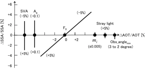
We show the results of the sensitivity tests in Fig. 2. In the cases where we changed the initial value of the imaginary part of the refractive index, added stray light, and changed the minimum observable scattering angle, there are no sig-nificant differences in the SSA from the case without errors, with the differences being less than 1 %. On the other hand, in the case where we assumed an error forAg, SVA, andF0, the result shows differences in the SSA relative to the case without errors.
Figure 3 shows the difference in SSA at a wavelength of 0.5 µm between cases with and without error, defined as {[SSA (with error)−SSA (no error)]/[SSA (no error)]}. When we assumed errors of −50 % (−0.1), −5 %, and
−5 % forAg, SVA, andF0, respectively, the differences in SSA were+3.7 %,+3.0 %, and+5.5 % at a wavelength of 0.5 µm. For the AOT at a wavelength of 0.5 µm, there was no difference, defined as{[AOT (error)−AOT (no error)]/[AOT (no errors)]}, when we introduced an error inAgand SVA, but there was a+2.8 % difference when we introduced an error inF0.
0.75 0.8 0.85 0.9 0.95 1
0.4 0.5 0.6 0.7 0.8 0.9 1 1.1
SS
A
Wavelength [µm]
ret_‐5%SVA ret_default ret_+5%SVA
0.75 0.8 0.85 0.9 0.95 1
0.4 0.5 0.6 0.7 0.8 0.9 1 1.1
SS
A
Wavelength [µm]
ret_‐5%F0 ret_default ret_+5%F0
0.75 0.8 0.85 0.9 0.95 1
0.4 0.5 0.6 0.7 0.8 0.9 1 1.1
SS
A
Wavelength [µm]
ret_‐50%Ag ret_default ret_+50%Ag
0.75 0.8 0.85 0.9 0.95 1
0.4 0.5 0.6 0.7 0.8 0.9 1 1.1
SS
A
Wavelength [µm]
ret_‐0.005Mi ret_default ret_+0.005Mi
0.75 0.8 0.85 0.9 0.95 1
0.4 0.5 0.6 0.7 0.8 0.9 1 1.1
SS
A
Wavelength [µm]
ret_obs_angle2deg ret_default
0.75 0.8 0.85 0.9 0.95 1
SS
A
Wavelength [µm]
ret_stray_light ret_default
Fig. 2. SSA values in the sensitivity experiments as a function of wavelength at 0.400, 0.500, 0.675, 0.870, and 1.02 µm.andNindicate the
results with an error or with a change to the parameter applied as described in the graph legends.shows the result without error or change
applied to the parameters. The following errors and changes were applied:±5 % toF0,±5 % to SVA,±50 % toAg,±0.005 to the initial
value of the imaginary part of the refractive index, an increase in the diffused intensity at scattering angle 3◦by 5 % at each wavelength (stray
light), and a decrease in the minimum observable scattering angle of the sky radiometer from 3◦to 2◦.
mi
(±0.005)
∆
∆
Fig. 3. Summary of the errors in retrieved SSA in percentage at a
wavelength of 0.5 µm in the sensitivity experiments. The horizontal axis shows parameters that are applied errors or changes, and also
shows the error from the true value in retrieved AOT (1AOT/AOT).
The longitudinal axis is the error from the true value in retrieved
SSA. SVA is the solid view angle;Ag, the ground surface albedo;
F0, the calibration constant;mi, imaginary part of refractive
in-dex; Obs anglemin, the minimum observable angle. Applied error
or changes are in parentheses.
the causes of error in the SSA. Although the value ofAg de-pends on wavelength and ground conditions, the value used in data processing at the SKYNET data center is set to 0.1 for each wavelength. As for the SVA value, it is determined by the disk scan method, called the Sun scanning method in Nakajima et al. (1996). At present, the disk scan in SKYNET varies according to the observation site. For some sites, the observation software is set to perform a disk scan periodi-cally at intervals of a few days (e.g., 1 week or 10 days) at a certain time (e.g., 11:00 a.m. LT). However, for other sites disk scan data are missing for long periods (e.g., more than 1 yr). The stability of the estimated SVA time series indicates that possible errors included in the SVA are within 5–6 % because of the lens degradation and color aberration of the
0 0.5 1 1.5 2 2.5 3
0 0.2 0.4 0.6 0.8 1 1.2
SS
A err
or [%]
AOT (0.5µm)
Fig. 4. The absolute value of the averaged error in SSA at a
wave-length of 0.5 µm on percentage for the value of AOT, 0.05, 0.1, 0.2, 0.3, 0.4, 0.5, and 1.0. The bar indicates the standard deviation.
single lens used in the radiometer, which produces an error of
∼3 % in the SSA. SKYNET SVA in the standard analysis is calculated by the point source method (Nakajima et al., 1996) by using disk scan data measured at the interval of few days (e.g., 1 week or 10 days) at certain time (e.g, 11:00 a.m. in the morning), and is one month averaged data of SVA of which deviation is within 10 %. However, for some sites, disk scan data are missing for a long time (more than 1 yr). We took standard deviation of the error of determined SVAs at Pune and Beijing, and the standard deviation is within 5–6 %. We therefore put 5 % error in SVA for the test. For the error 3 % in SSA due to SVA error, it was found from the result of the sensitivity test that 5 % error in SVA occurs about 3 % error in SSA.
surface albedo Ag, calibration constant F0, and SVA 1 are given as 0.2, 1, and 2.5×10⁻⁴str, respectively, at a wavelength of 0.5 µm. The solar zenith angle is given at θ0=60◦. We examined the error in retrieved SSA when AOT is 0.05, 0.1, 0.2, 0.3, 0.4, 0.5, and 1.0, for five aerosol mod-els such as dust-like and rural aerosol types in the WCP re-port (Deepak and Gerber, 1983), and soluble, water-insoluble, and mineral accumulate aerosol types (Hess et al., 1998). As shown in Fig. 4, the averaged error between the retrieval value and true value of the SSA, which is defined as h|SSA(retrieval)−SSA(true)|/SSA(true)i, is about 1 % when the value of AOT is larger than 0.2 or 0.3, and the er-ror of the SSA and its variation (standard deviation in the figure) became larger with decreasing AOT values. There-fore, it could be said that the condition of low AOT af-fects the retrieval accuracy of SSA, especially when AOT is less than 0.2. It is reported that the error in retrieved SSA decreases with increasing aerosol optical thickness for AERONET (Dubovik et al., 2000). We found a similar ten-dency for SKYNET sky radiometer data analysis in this pa-per. The amount of aerosols, AOT, in the atmosphere easily varies in one day, and in many places the AOT values are lower than 0.2 or 0.3 at a wavelength of 0.5 µm almost every day. Therefore, in the low AOT case, we should note that it is difficult to retrieve an accurate SSA by using the present algorithm.
In conclusion, it is possible that the errors associated with Agand SVA, and the amount of aerosols in the atmosphere, are the causes of error in the SSA. However, the errors in evaluating SSA due to these parameters and the low AOT condition will be less than 5 %, and these errors should cause both underestimation and overestimation of SSA, so it is difficult to explain the reported overestimation for all these sites.
2.3 Sensitivity tests for difference in inversion
algorithms
SKYRAD.pack version 4 utilizes the Phillips-Twomey method to minimize the cost function given in Eq. (5) to determine aerosol parameters, such as the volume size dis-tribution and refractive index, as described in Section 2.1. In this method, the a priori information for stabilizing the ill-conditioned Fredholm integral equation is the smoothness of the retrieved SDF given by the B2matrix. On the other hand, similar a priori constraints can be applied in the framework of a statistical estimation approach, for example, as imple-mented in AERONET retrieval via a non-linear maximum likelihood method defined in the logarithmic space of the re-trieved variables SDF andm˜. Here, we base our approach on the MLM method as defined by Rodgers (2000). This method is based on the Bayesian theory.
p (x|f)=p (f|x) p (x)
p (f) , (6)
wherep is the probability density function and is defined as the Gaussian distribution; andx andf denote state and measurement vectors, respectively. In the MLM method,x
is chosen so that the posterior probabilityp (x|f)becomes maximum under the condition that a priori information is al-ready given. Organizing this non-linear equation such that p (x|f)=max, we obtain the following equation in the tan-gential space to be solved by a Newtonian method:
xk+1=xk+
UTkS−e1Uk+S−a1
−1
h
UTkS−e1(f−fk)−S−a1(xk−xa)
i
, (7)
where xk is the solution at the k-th iteration step; fk=
f(xk), an observation modeled usingxk; xa, the a priori value ofx; Se, the measurement error covariance matrix; Sa, the covariance matrix defined by a priori and state values,
Sa=
(x−xa) (x−xa)T
; and U, the Jacobi matrix,∂f/∂x. Further, it should be noted that in a manner similar to the AERONET approach (Dubovik and King, 2000), we used a logarithmic scale for the volume size distribution and com-plex refractive index to prevent x from having a negative value.
Thus, analogous to the AERONET retrieval approach, the retrieval algorithm used in version 5 allows rigorous retrieval of both the aerosol size distribution and the spectral complex refractive index. At the same time, some differences remain between the version 5 and AERONET retrieval methods. Specifically, AERONET retrieval does not use the MLM of Rodgers (2000) corresponding to Eq. (7). Instead, it uses the multi-term LSM (Least Square Method) described in papers by Dubovik and King (2000), Dubovik (2004), and Dubovik et al. (2011). Similarly to Rodgers’ method, multi-term LSM relies on a statistical estimation approach; however, it differs by allowing simultaneous use of multiple a priori constraints. For example, it can include both a priori constraints on the smoothness of retrieved functions and a priori estimates of the state vector. Specifically, instead of Eq. (7), the solution of the AERONET algorithm is expressed as follows:
xk+1=xk+
UTkS−e1Uk+γ1+S−a1
−1
h
UTkS−e1(f−fk)−γ1xk−S−a1(xk−xa)
i , (8) whereis the smoothness matrix. This is used by Dubovik and King (2000) to apply different smoothness constraints on the size distribution (v (r)), on the spectrally dependent real part of the complex refractive index (n (λ)), and on the spec-trally dependent imaginary part of the complex refractive in-dex (m (λ)). The state vector retrieved by the AERONET al-gorithm can be denoted byxT =(xv;xn;xm;xsph)T, where
xvis a vector includingNv=22 values ofv (ri);xn, a vec-tor includingNλvalues ofn λϕ
;xm, a vector includingNλ values ofm λϕ
γ1=
γvv 0 0 0
0 γnn 0 0
0 0 γkk 0
0 0 0 0
, (9)
where v=BTvBv, n=BTnBn, k=BTkBk are smooth-ness matrices of different dimensions Nv×Nv, Nλ×Nλ, andNλ×Nλ accordingly, defined via the matrices Bv, Bn,
Bmof coefficients for estimating the corresponding deriva-tives. Specifically, Dubovik and King (2000) constrain the third derivatives ofv (r), the first derivatives of n (λ), and the second derivatives ofm (λ). It should be noted that ma-trix Bvis analogous to the matrix B used in Eq. (5) and de-fined as prescribed by Phillips (1962) and Twomey (1963); however, matrices Bn and Bk are slightly more complex because they are defined for non-equidistant discretization pointsλϕ(λϕ+1−λϕ6=const). The explicit definition of such matrices, as well as the definition of the corresponding La-grange parameters γ in Eq. (8), is given by Dubovik and King (2000) and explained in detail by Dubovik et al. (2011). Thus, the solution given by Eq. (8) minimizes the following cost function:
e2∼(f−fk)TS−e1(f−fk)+xTvvxv+xTnnxn
+xTmmxm+(xk−xa)TS−a1(xk−xa) . (10)
It is important to note that the AERONET algorithm uses a priori estimatesxaonly for two retrieved parameters{x}1
and{x}22 corresponding to the values of the retrieved size distribution of the smallest size class (r=0.05 µm) and the largest size class (r=15 µm), i.e., the matrix Sahas all zero elements except for the first and 22nd elements of the diag-onal, i.e.,{S}1 1and{S}22 22. This constraint was introduced by Dubovik et al. (2006) to avoid unrealistically increasing tails of size distribution appearing due to the very low sensi-tivity of sky radiometer observations to very small and very large particles. This constraint has a rather “cosmetic” ob-jective because, practically, it does not affect the minimum value of the cost function and, as was shown by Dubovik et al. (2000), the retrieval errors for size distribution tails are very high. At the same time, constraining the size distribu-tion tails to small values may give the wrong impression of an absence of very large and very small particles. The correct interpretation should state that there are very large and very small particles that make a contribution sufficient to change the values of the cost function (while the volume of those particles, in principle, cannot be negligible compared to the volume of the rest of the particles).
The values of{xa}22are given by AOT(0.44)×0.002. The initial guess for the size distribution is chosen as a straight line with values AOT(0.44)×0.01; for the refractive index, the initial guess is spectrally independent with values n=
1.45 andm=0.005.
In order to study whether the reported SSA differences can originate from the difference between the inversion algo-rithms of SKYNET and AERONET, we performed various test simulations with SKYRAD.pack version 4 and a new version 5, which has been developed using the algorithm that is explained above and is closer to the AERONET algorithm. Version 5 uses an a priori SDF of a bimodal log-normal func-tion,
v(r)=
2 X
n=1
Cnexp[− 1 2(
lnr−lnrmn lnSn
)2], (11)
withrm1=0.1 µm,rm2=2.0 µm,S1=0.4,S2=0.8,C1= 1.0×10⁻¹², and C2=1.0×10⁻¹² following reported cli-mate values (Higurashi et al., 2000). For a priori esticli-mates of the real part (n)and the imaginary part (m)of the refrac-tive index, we usually setn=1.5 andm=0.005, which are spectrally independent values. One of the key differences be-tween version 4 and version 5 is that version 5 uses a priori estimation, but version 4 does not.
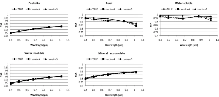
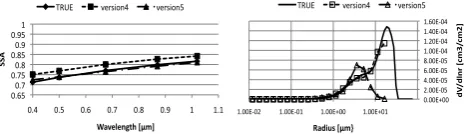
We first performed numerical tests by using Rstar-6b with two aerosol models incorporated in Rstar-6b, i.e., the dust-like and rural aerosol types in the WCP report (Deepak and Gerber, 1983), and three other aerosol models of Hess et al. (1998), i.e., water-soluble, water-insoluble, and mineral accumulate aerosol types, and we set AOT = 0.5 for each case. As shown in Figs. 5 and 6, the differences for the re-trieved SSA are found to be less than 0.01, and there were not large differences for the SDF. Among various other tests, we found one case in which a noticeable difference exists between version 4 and version 5, as shown in Fig. 7. In this case, we assumed that a tested true SDF includes a large amount of coarse particles of the dust-like aerosol type with radius greater than 10 µm. The figure shows that version 4 could retrieve the SDF relatively well, including the coarse mode, in comparison with version 5, because the smooth-ness condition given by Eq. (5) allows the retrieved SDF to be distributed beyond a 10 µm radius. On the other hand, ver-sion 5 underestimated the coarse mode of the SDF because of the strong SDF constraint condition given by Eq. (11) with a small model radiusrm2=2.0 µm for the coarse mode SDF. The value of the SSA is then underestimated to compensate the reduced light absorption by coarse particles. Although not shown in a figure, we found no significant error in the retrieved AOT because the inversion process did not bring about a large change in the retrieved direct solar radiation. As discussed later, an enhanced coarse mode SDF is possibly required for several dust storm cases (Chepil, 1957; Gillette et al., 1978; and Feng et al., 2007). The test indicates that version 4 can retrieve accurate SSA values in comparison to version 5 in this case. It is possible that version 5 may un-derestimate the SSA value because of the constraint on the SDF.
!"#$%!"&% !"&$%!"'% !"'$%!"(% !"($%)%
!"*% !"$% !"#% !"&% !"'% !"(% )% )")%
!!
"#
$%&'(')*+,#-./0#
12345(64'#
+,-.% /012345*% /012345$%
!"&% !"&$%!"'% !"'$% !"(% !"($%)%
!"*% !"$% !"#% !"&% !"'% !"(% )% )")%
!!
"#
$%&'(')*+,#-./0#
728%(#
+,-.% /012345*% /012345$%
!"&% !"&$%!"'% !"'$% !"(% !"($%)%
!"*% !"$% !"#% !"&% !"'% !"(% )% )")%
!!
"#
$%&'(')*+,#-./0#
$%+'8#39(2:('#
+,-.% /012345*% /012345$%
!"#$%!"&% !"&$%!"'% !"'$%!"(% !"($%)%
!"*% !"$% !"#% !"&% !"'% !"(% )% )")%
!!
"#
$%&'(')*+,#-./0#
$%+'8#6)39(2:('#
+,-.% /012345*% /012345$%
!"&% !"&$%!"'% !"'$%!"(% !"($% )%
!"*% !"$% !"#% !"&% !"'% !"(% )% )")%
!!
"#
$%&'(')*+,#-./0#
;6)'8%(#<9%83'#
+,-.% /012345*% /012345$%
Fig. 5. SSA values derived by SKYRAD.pack version 4 and version 5 algorithms for the dust-like and rural aerosol types of WCP (Deepak
and Gerber, 1983) and for the water soluble, water insoluble, and mineral accumulate aerosol types of Hess et al. (1998).
!"!!#$!!% &"!!#'!(% )"!!#'!(% ("!!#'!(% *"!!#'!(% +"!!#'!,% +"&!#'!,%
+"!!#'!&% +"!!#'!+% +"!!#$!!% +"!!#$!+%
!"
#!$%&'()*+#
)*,-'
./!012'(3*-' 40%5&/$')6/&25'
-./#% 0123456)% 0123456,%
!"!!#$!!% +"!!#'!,% &"!!#'!,% 7"!!#'!,% )"!!#'!,% ,"!!#'!,% ("!!#'!,% 8"!!#'!,% *"!!#'!,%
+"!!#'!&% +"!!#'!+% +"!!#$!!% +"!!#$!+%
!"
#!$%&'()*+#
)*,-'
./!012'(3*-' 7/85&'0%26$9$5'
-./#% 0123456)% 0123456,%
!"!!#$!!% +"!!#'!,% &"!!#'!,% 7"!!#'!,% )"!!#'!,% ,"!!#'!,% ("!!#'!,% 8"!!#'!,% *"!!#'!,%
+"!!#'!&% +"!!#'!+% +"!!#$!!% +"!!#$!+%
!"
#!$%&'()*+#
)*,-'
./!012'(3*-' :128;$0<5'
-./#% 0123456)% 0123456,%
!"!!#$!!% ,"!!#'!8% +"!!#'!(% +",!#'!(% &"!!#'!(% &",!#'!(% 7"!!#'!(% 7",!#'!(% )"!!#'!(% )",!#'!(%
+"!!#'!&% +"!!#'!+% +"!!#$!!% +"!!#$!+%
!"
#!$%&'()*+#
)*,-'
./!012'(3*-' .1&/$'
-./#% 0123456)% 0123456,%
!"!!#$!!% +"!!#'!(% &"!!#'!(% 7"!!#'!(% )"!!#'!(% ,"!!#'!(% ("!!#'!(%
+"!!#'!&% +"!!#'!+% +"!!#$!!% +"!!#$!+%
!"
#!$%&'()*+#
)*,-'
./!012'(3*-' 7/85&'26$9$5'
-./#% 0123456)% 0123456,%
Fig. 6. SDF values derived by SKYRAD.pack version 4 and version 5 for the dust-like and rural aerosol types of WCP (Deepak and Gerber,
1983) and for the water soluble, water insoluble, and mineral accumulate aerosol types of Hess et al. (1998).
at a wavelength of 0.5 µm by using Rstar-6b, and com-pared it with and without a cut above 10 µm for the SDF. We used dust-like aerosol model incorporated in Rstar-6b, which is described by a mono-modal log-normal SDF with mode radius 6.0 µm. The AOT set-ting at 0.5 µm is 0.5. Figure 8 shows the difference between the relative intensity with and without a cut above 10 µm for the SDF {1R= [R(cut above 10 µm)−
R(no cut above 10 µm)]/R(no cut above 10 µm)}. The mini-mum scattering angle is 3 degrees. From this result, the lack of a large coarse part in the SDF causes overestimation of sky radiance at all observation angles. The intensity of for-ward scattering near 0 degree increases with increase in par-ticle size, but the simulation shows that the diffused inten-sity without over 10 µm particles is larger than that with over 10 µm particles in the region of measured scattering angles (>3 degree) in the same condition of AOT. Hence, a lack
of large particles (>10 µm radius) causes “overestimation” of radiance. It is likely that version 5 works to decrease the SSA value to dim the sky radiance in the calculation when a tight constraint on the SDF for particles with radius over 10 µm is applied. The constraint that is used in AERONET data processing for suppressing the concentration of parti-cles corresponding to the largest class (r=15 µm) may have a similar effect. However, there are other differences, e.g., a priori estimates, other constraints, or determination of a co-variance value, etc. Therefore, we need further investigation of this finding.
!"#$ !"#%$ !"&$ !"&%$ !"'$
!"($ !"%$ !")$ !"#$ !"&$ !"'$ *$ *"*$
!!
"#
$%&'(')*+,#-./0# 1%2*'#345+# +,-.$ /012345($ /012345%$
!"!!.6!!$ *"!!.7!%$ 8"!!.7!%$ 9"!!.7!%$ ("!!.7!%$ %"!!.7!%$ )"!!.7!%$ #"!!.7!%$
*"!!.7!8$ *"!!.7!*$ *"!!.6!!$ *"!!.6!*$
36
73()2#-8/97
8/:0#
;%3<45#-./0#
+,-.$ /012345($ /012345%$
Fig. 7. Values of SSA (left panel) and SDF (right panel) for the
enhanced coarse mode case. Solid, dashed, and dashed-dotted lines represent true values, retrieved values from version 4, and retrieved values from version 5, respectively.
0 1 2 3 4 5 6 7
0 10 20 30 40 50 60 70 80 90 100 110 120 130
Diff
er
ence of r
ela-v
e r
adiance [%]
Azimuth angle [degree]
0.5µm
Fig. 8. The percentage difference of the relative radiances at 0.5 µm
for each scattering angle between SDFs with and without particles over 10 µm in radius.
cirrus particles, respectively. We set AOT = 0.5 for dust-like particles and an optical thickness of 0.1 for ice particles at a wavelength of 0.5 µm. For the other conditions, we chose US-standard atmosphere and set the solar zenith angle at θ0=60◦. The ground surface albedoAg, calibration constant F0, and solid view angle (SVA)1are given as 0.2, 1, and 2.5×10⁻⁴str, respectively, at wavelengths of 0.4, 0.5, 0.675, 0.84, and 1.02 µm. In simulation data, we consider the for-ward scattering light that measured as a direct solar irradi-ance in the field of view, and SKYNET retrieval algorithm has the process to remove this overestimation of direct irra-diance.
In this case, the SDF consists of the first mode due to aerosol particles and a second coarse mode due to cirrus par-ticles, as shown in Fig. 9.
The inversion result shows that version 4 retrieved the SDF, including contaminating cirrus particles larger than 10 µm, but version 5 successfully filtered out the cirrus par-ticles by the constraint of a reduced SDF for parpar-ticles with radius greater than 10 µm. As a result, the SSA value re-trieved by using version 5 became closer to the true value of SSA. This test indicates that cirrus contamination can cause a serious overestimation of SSA from SKYNET as reported, whereas SSA retrieved by using version 5 is robust and with-out significant error.
!"!!#$!!% &"!!#'!(% )"!!#'!(% *"!!#'!(% +"!!#'!(% ,"!!#'!)% ,"&!#'!)% ,")!#'!)% ,"*!#'!)%
,"!!#'!&% ,"!!#'!,% ,"!!#$!!% ,"!!#$!,%
!"
#!$%&'()*+#
)*,-'
./!012'(3*4'
-./#% 0123456)% 0123456(%
!"*(%!"7% !"7(%!"+% !"+(%!"8% !"8(%,%
!")% !"(% !"*% !"7% !"+% !"8% ,% ,",%
55
6'
7/89$9%:;<'(3*-' =0&&12')>%;/*0%/?>%'
-./#% 0123456)% 0123456(%
Fig. 9. Values of SSA (left panel) and SDF (right panel) for the
cirrus contamination case. Solid, dashed, and dashed-dotted lines represent true values, retrieved values from version 4, and retrieved values from version 5, respectively.
3 Analysis of observation data
3.1 Case studies
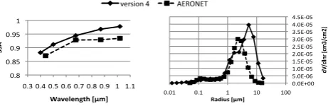
To investigate whether enhanced coarse dust particles and/or cirrus contamination can affect the real SSA retrieval, we an-alyzed SKYNET data at the Pune site (18.616◦N/73.800◦E) in India, which is one of the collocated sites of SKYNET and AERONET radiometers. We used the data for 23 Octo-ber 2008, when cirrus was detected over the Pune site by the CALIPSO lidar, as illustrated in Fig. 10. As shown in Fig. 11, it is found that version 4 retrieved an SDF with an enhanced coarse mode that seems to be a cirrus particle contribution. On the other hand, version 5 gave an SDF without a large coarse mode as an a priori value. Values of SSA from version 4 were larger than those from version 5 for the reason we pro-posed in the preceding section. This result is consistent with the result of numerical experiments on cirrus contaminations, so it is likely that, in this case, the SSA retrieved by ver-sion 4 was overestimated because of cirrus contamination. In the period of cirrus contamination, AERONET consistently eliminates the data through their symmetry check of the two sides of the almucantar scan (Holben et al., 2006), whereas the SKYNET scan only has one side of the almucantar and thus cannot use such symmetry quality check.
Fig. 10. Aerosol detection over Pune by CALIPSO lidar. This panel indicates a cirrus cloud case (23 October 2008, 08:36:00.2 to 08:49:28.9
UTC), for aerosol types of dust (yellow), polluted continental aerosol (red), polluted dust (brown), clean continental aerosol (green), and smoke (black). The data were taken from the NASA CALIPSO web site (http://www-calipso.larc.nasa.gov/products/lidar/browse images/ production/).
!"!#$!!% &"!#'!(% )"!#'!(% *"!#'!(% +"!#'!(% ("!#'!(% ,"!#'!(% -"!#'!(% ."!#'!(% /"!#'!(% &"!#'!+%
!"!&% !"&% &% &!%
!"
#!$%&'()*+#
)*,-''
./!012'(3*-''
!"!#$!!% &"!#'!,% )"!#'!,% *"!#'!,% +"!#'!,% ("!#'!,% ,"!#'!,% -"!#'!,% ."!#'!,% /"!#'!,% &"!#'!(%
!"!&% !"&% &% &!%
!"
#!$%&
'()*+#
)*,-'
./!012'(3*-'
!"-% !"-(% !".% !".(% !"/% !"/(% &%
!"*% !"+% !"(% !",% !"-% !".% !"/% &% &"&%
40%5$6'2)
/76&0%5'/$86!9'
:/;6$/%5<='(3*-'
0123456%+% 0123456%(%
!"-% !"-(% !".% !".(% !"/% !"/(% &%
!"*% !"+% !"(% !",% !"-% !".% !"/% &% &"&%
40%5$6'2)
/76&0%5'/$86!9'
:/;6$/%5<='(3*-'
!"!#$!!% &"!#'!(% )"!#'!(% ("!#'!(% *"!#'!(% +"!#'!,% +"&#'!,% +")#'!,% +"(#'!,%
!"!+% !"+% +% +!%
!"
#!$%&'()*+#
)*,-'
./!012'(3*-'
-./0123%)% -./0123%,% 4#567#8%
Fig. 11. SSA (left panel) and SDF (right panel) at Pune retrieved by
version 4 (solid line) and by version 5 (dashed line) for a cirrus case (23 October 2008, 08:36:00.2 to 08:49:28.9 UTC).
those from SKYNET, consistent with the result of numeri-cal experiments in the previous section. Since cirrus cloud was not detected from the lidar, it is likely that the differ-ence in the two products was caused by the differdiffer-ence in the inversion method. However, we cannot conclude this point, because there are several differences between the AERONET algorithm and SKYRAD.pack, e.g. input parameters such as surface albedo, instrument calibration method and scanning system. Therefore, more studies, including validation of the SDF, will be needed in the future.
3.2 Development of a quality control algorithm
In this section, we mention and suggest an approach to the issue of quality control of observation data and cloud screen-ing.
The present standard process of quality control in SKYNET applies a retrieval error between observations and calculated theoretical values by using retrieval values,σobs,
σobs= s
We X
i
τλi/τ
meas
λi −1 2
+WP
X
i X
j h
Rλi 2j
/Rmeasλ
i 2j
−1
i2
,(12)
Backscattering intensity (532nm) Int1064/Int532
Lidar Observation at Beijing
Depolarization ratio (532nm)
Fig. 12. Lidar observation at Beijing by NIES lidar from 14:00 UTC
to 15:00 UTC on 14 April 2004. The left panel, center panel, and right panel show backscattering intensity at wavelength 0.532 µm, depolarization ratio at wavelength 0.532 µm, and the color ratio of
scattering intensities atλ=1.064 µm and 0.532 µm, respectively.
The arrows indicate the time that we checked the SKYNET data (14 April 2004, 09:06:17 UTC).
where (τλmeas i and R
meas
λi )and (τλi and Rλi)are measured and retrieved observation vectors for the AOT and relative sky radiance defined by Eqs. (1)–(3) at measurement wave-lengths. Now we setWe=WP =1/Ntotal, whereNi,Nj, and Ntotal=Ni+Ni×Njindicate the number of measured wave-lengths, scattering angles, and their total, respectively. In the present standard retrieval process in SKYNET, we remove the data if the value ofσobsis larger than 0.2.
M. Hashimoto et al.: Development of a new data-processing method for SKYNET 2733 !"#$ !"#%$ !"&$ !"&%$ '$
!"($!")$!"%$!"*$!"+$!"#$!"&$ '$ '"'$
!! "# $%&'(')*+,#-./0# !"!#$!!% &"!#'!(% )"!#'!&% )"&#'!&% *"!#'!&% *"&#'!&% +"!#'!&% +"&#'!&% ,"!#'!&% ,"&#'!&%
!"!)% !")% )% )!% )!!%
!" #!$%&'()*+# )*,-' ./!012'(3*-' ,-**$+(."/%)0-/)1"/(! 2)*3&('$+%! !"#$ !"#%$ !"&$ !"&%$ !"'$ !"'%$ ($
!")$ !"%$ !"*$ !"#$ !"&$ !"'$ ($ ("($
!! "# $%&'(')*+,#-./0# 12)'3%(#45%36'# +,-.$ /012345)$ /012345%$
4&*+-"/5!"""67!(
!"#$ !"#%$ !"&$ !"&%$ !"'$ !"'%$ ($
!")$ !"%$ !"*$ !"#$ !"&$ !"'$ ($ ("($
!! "# $%&'(')*+,#-./0# 12)'3%(#45%36'# +,-.$ /012345)$ /012345%$ !"#$ !"#%$ !"&$ !"&%$ !"'$ !"'%$ ($
!")$ !"*$ !"%$ !"+$ !"#$ !"&$ !"'$ ($ ("($ ,-./012$*$ 3456748$
Fig. 13. SSA and SDF in Beijing retrieved by version 4 (solid line;
14 April 2004, 09:00:00 UTC), and by AERONET (dashed line; 14 April 2004, 09:06:17 UTC).
kept in the clear sky data group. Secondly, the spectral depen-dency behaviors of aerosols and cloud, which use a spectral variability cloud screening algorithm (Kaufman et al., 2006) as a reference, are used (Eq. 13). The 15-min data are used.
1τ870 nm−1τ400 nm(τ870 nm/τ400 nm) >0.0075+0.03τ675 nm. (13)
Here,τ is an observation value,1τ is the maximum devi-ation of neighboring data, and the subscript notdevi-ation indi-cates wavelength in nanometers. The numbers “0.0075” and “0.03” correspond to a noise error and the influence of re-fractive humidity, respectively. This criterion is applied to the data in the cloud-affected data group, and the data are regarded as cloud-affected data if the data fail to meet the criterion. Finally, statistical analysis tests in Eq. (14) are performed to remove outliers that pass the first and second checks, in an approach similar to Smirnov et al. (2000). τλ(max)−τλ(min)≥0.02, whenτ <0.7. (14) This process is applied to the triplet data in a minute.
The present cloud screening relies heavily on the global flux test and needs global irradiance data but, almost uni-formly, the observation sites in SKYNET do not conduct an observation of solar irradiance. Furthermore, cirrus contami-nation data are difficult to remove as cloud-affected data.
On the basis of the result of numerical experiments and real data analysis, we develop a quality control (QC) algo-rithm in this subsection to estimate more accurate SSA.
We drop data according to the following three conditions: (C1) the AOT is less than 0.4 at a wavelength of 0.5 µm, us-ing the AERONET Level 2.0 QC algorithm, because the re-trieval error in SSA rapidly increases with decreasing AOT (Dubovik et al., 2000). AERONET uses 0.44 µm as the wave-length for this algorithm, but there is no observation at a wavelength of 0.44 µm in SKYNET. Therefore, instead of AOT(0.44 µm), we use AOT(0.5 µm). (C2) We then reject data with a large deviation of the retrieved observation vector from the measured observation vector by using Eq. (12). We definedσobs=0.07 as a threshold for data rejection, through semi-empirical judgment of measurement errors found in the data analysis of large volume data sets in the past, including instrumental errors and errors in radiative transfer modeling
!"#$ !"#%$!"&$ !"&%$!"'$ !"'%$($
($ )$ *$ +$ %$ ,$ #$ &$ '$ (!$ (($ ()$
!"#$%&'() *+&,"#$'*%-&./' 0/#12' 3&4/,&'(),&&#"#$'567#&8' !"#$ !"#%$!"&$ !"&%$!"'$ !"'%$($
($ )$ *$ +$ %$ ,$ #$ &$ '$ (!$ (($ ()$
!"#$%&'() *+&,"#$'*%-&./' 0/#12' 34&,'(),&&#"#$'-5'678'698'6:';<=#&>' !"#$ !"#%$!"&$ !"&%$!"'$ !"'%$($
($ )$ *$ +$ %$ ,$ #$ &$ '$ (!$ (($ ()$
!"#$%&'() *+&,"#$'*%-&./' 0/#12' 3&4/,&'(),&&#"#$'567#&8' !"#$ !"#%$!"&$ !"&%$!"'$ !"'%$($
($ )$ *$ +$ %$ ,$ #$ &$ '$ (!$ (($ ()$
!"#$%&'() *+&,"#$'*%-&./' 0/#12' 345'')61'789:;<=5'>'9:?'8@6#&5' !"#$ !"#%$!"&$ !"&%$!"'$ !"'%$($
($ )$ *$ +$ %$ ,$ #$ &$ '$ (!$ (($ ()$
!"#$%&'() *+&,"#$'*%-&./' 0/#12' 345')61'&,,'7'89':;6#&5' !"#$ !"#%$!"&$ !"&%$!"'$ !"'%$($
($ )$ *$ +$ %$ ,$ #$ &$ '$ (!$ (($ ()$
!"#$%&'() *+&,"#$'*%-&./' 0/#12' 345')61'7689&.'.:;.%#,'<=6#&5' !"#$ !"#%$!"&$ !"&%$!"'$ !"'%$($
($ )$ *$ +$ %$ ,$ #$ &$ '$ (!$ (($ ()$
!"#$%&'() *+&,"#$'*%-&./' 0/#12' 3&4/,&'(),&&#"#$'567#&8' !"#$ !"#%$!"&$ !"&%$!"'$ !"'%$($
($ )$ *$ +$ %$ ,$ #$ &$ '$ (!$ (($ ()$
!"#$%&'() *+&,"#$'*%-&./' 0/#12' 345'')61'789:;<=5'>'9:?'8@&"A"#$5' !"#$ !"#%$!"&$ !"&%$!"'$ !"'%$($
($ )$ *$ +$ %$ ,$ #$ &$ '$ (!$ (($ ()$
!"#$%&'() *+&,"#$'*%-&./' 0/#12' 3&4/,&'(),&&#"#$'53&"6"#$7' !"#$ !"#%$!"&$ !"&%$!"'$ !"'%$($
($ )$ *$ +$ %$ ,$ #$ &$ '$ (!$ (($ ()$
!"#$%&'() *+&,"#$'*%-&./' 0/#12' 34&,'(),&&#"#$'-5'678'698'6:';<&"="#$>' !"#$ !"#%$!"&$ !"&%$!"'$ !"'%$($
($ )$ *$ +$ %$ ,$ #$ &$ '$ (!$ (($ ()$
!"#$%&'() *+&,"#$'*%-&./' 0/#12' 345')61'7689&.'.:;.%#,'<=&"7"#$5' !"#$ !"#%$!"&$ !"&%$!"'$ !"'%$($
($ )$ *$ +$ %$ ,$ #$ &$ '$ (!$ (($ ()$
!"#$%&'() *+&,"#$'*%-&./' 0/#12' 345')61'&,,'7'89':;&"<"#$5' !"#$ !"#%$!"&$ !"&%$!"'$ !"'%$($
($ )$ *$ +$ %$ ,$ #$ &$ '$ (!$ (($ ()$
!"#$%&'()
*+&,"#$'*%-&./'
0/#12' 3&4/,&'(),&&#"#$'53&"6"#$7'
Fig. 14. Monthly mean and standard deviation of SSA atλ=0.5 µm before (black) and after (white) screening by all conditions of C1, C2, and C3, and after screening by each condition (C1, C2 or C3) individually (each screened result by C1, C2, or C3 are shown by red, blue, and green, respectively). The top panel shows the result at Pune in 2008 and the bottom panel shows the result at Beijing in 2004.
and optical modeling of scatters. (C3) We then pose a condi-tion regarding the magnitude of the coarse mode of the SDF given by Eq. (3c).
Cv×v (2.4 µm) <max{v (7.7 µm) , v (11.3 µm) , v (16.5 µm)}, (15)
whereCvis a threshold coefficient to be determined for opti-mum rejection of cirrus contamination. This condition is set to warn the system that the retrieved SDF from version 4 in-cludes a large volume of coarse mode particles larger than 10 µm. We setCv=2 from the analysis of data at the Pune and Beijing sites, which enables rejection of most cirrus con-tamination cases. There were some dust cases that also have a large coarse mode, but the magnitude of the coarse mode is lower than that of cirrus contamination and can pass through this condition. The value ofCvis determined from one year of data of the Pune and Beijing sites. It will be necessary for future work to determine this value after we collect more dust day data and cirrus contamination data.
!" !#$" !#%" !#&" !#'"
!#("!#(%"!#('"!#()"!#(*"!#*"!#*%"!#*'"!#*)"!#**"!#+"!#+%"!#+'"!#+)"!#+*"$"
!"#$%& !" !#$" !#%" !#&" !#'"
!#("!#(%"!#('"!#()"!#(*"!#*"!#*%"!#*'"!#*)"!#**"!#+"!#+%"!#+'"!#+)"!#+*"$"
'(")(*+(#& !"!## !"$## !"%## !"&## !"'##
!"(#!"(%#!"('#!"()#!"(*#!"*#!"*%#!"*'#!"*)#!"**#!"+#!"+%#!"+'#!"+)#!"+*#
$# !"#$%&'()$*$+,-& !"!## !"$## !"%## !"&## !"'##
!"(#!"(%#!"('#!"()#!"(*#!"*#!"*%#!"*'#!"*)#!"**#!"+#!"+%#!"+'#!"+)#!"+*#
$# .)"/)01)#&'()$*$+,-& !"!!## !"$!## !"%!## !"&!## !"'!##
!"(#!"(%#!"('#!"()#!"(*#!"*#!"*%#!"*'#!"*)#!"**#!"+#!"+%#!"+'#!"+)#!"+*#$#
!"#$%&'()*$ !"!## !"$## !"%## !"&## !"'##
!"(#!"(%#!"('#!"()#!"(*#!"*#!"*%#!"*'#!"*)#!"**#!"+#!"+%#!"+'#!"+)#!"+*#$#
+,-./)0$%&'()*$ !" !#$" !#%" !#&" !#'"
!#("!#(%"!#('"!#()"!#(*"!#*"!#*%"!#*'"!#*)"!#**"!#+"!#+%"!#+'"!#+)"!#+*"$"
!"#$ !" !#$" !#%" !#&" !#'"
!#("!#(%"!#('"!#()"!#(*"!#*"!#*%"!#*'"!#*)"!#**"!#+"!#+%"!#+'"!#+)"!#+*"$"
%&'()*+$ !"#$%&'()*++&,"#$'*%-&./! 0,&12&#)3'."(+,"-2+"/# ! !45678'-&9/,&'(),&&#"#$! !45678'*9+&,'(),&&#"#$! !"!## !"$## !"%## !"&## !"'## !"(## !")##
!"*#!"*%#!"*'#!"*)#!"*+#!"+#!"+%#!"+'#!"+)#!"++#!",#!",%#!",'#!",)#!",+#$# !"!## !"$## !"%## !"&## !"'## !"(## !")##
!"*#!"*%#!"*'#!"*)#!"*+#!"+#!"+%#!"+'#!"+)#!"++#!",#!",%#!",'#!",)#!",+#$# !"!## !"$## !"%## !"&## !"'## !"(## !")##
!"*#!"*%#!"*'#!"*)#!"*+#!"+#!"+%#!"+'#!"+)#!"++#!",#!",%#!",'#!",)#!",+#
$# !"!## !"$## !"%## !"&## !"'## !"(## !")##
!"*#!"*%#!"*'#!"*)#!"*+#!"+#!"+%#!"+'#!"+)#!"++#!",#!",%#!",'#!",)#!",+#
$#
:7;<678!
Fig. 15. Normalized frequency distributions of SSA from SKYNET
and AERONET in May and October at Pune and in April and September at Beijing. Upper and middle panels are for SKYNET SSA before and after data screening, respectively, and lower panel is the figure for AERONET SSA.
Fig. 16. Seven-day back trajectories on 11 May 2008,
12:00:00 UTC at Pune from the AERONET web site (NASA, http://croc.gsfc.nasa.gov/aeronet/).
By applying condition C3, the monthly mean SSA at Pune became lower than before screening, because the SSA val-ues that were very high or close to unity were removed by condition C3. On the other hand, the results at Beijing did not show a similar reduction in high SSA values. More de-tailed investigation of the results shows that the contribution of C2 is larger than those of C1 and C3 at both sites. This result indicates that theσobsvalue is useful for detecting ill-conditioned data caused by cirrus contaminations, horizon-tally and/or temporally inhomogeneous aerosol stratification, and so on.
Figure 15 shows the normalized frequency distribution of SSA values retrieved by the system with and without data screening by all three conditions, and also shows its value from AERONET. It is found from the figure that SSA vari-ability is significantly decreased after data screening. More-over, the frequency of cases of SSA values close to unity was noticeably reduced. In addition, the SSA values after data screening become closer to the values from AERONET than they were before the data screening.
!"#$ !"#%$ !"&$ !"&%$ '$
!"($ !")$ !"%$ !"*$ !"+$ !"#$ !"&$ '$ '"'$
!! "# $%&'(')*+,#-./0# !"!#$!!% &"!#'!(% )"!#'!&% )"&#'!&%
!"!)% !")% )% )!%
!" #!$%&'()*+# )*,-' !./!012'(3*-' !"#$ !"#%$ !"&$ !"&%$ !"'$ !"'%$ ($
!")$ !"*$ !"%$ !"+$ !"#$ !"&$ !"'$ ($ ("($ ,-./012$*$ 3456748$ !"#$ !"#%$ !"&$ !"&%$ '$
!"($ !")$ !"%$ !"*$ !"+$ !"#$ !"&$ '$ '"'$
!! "# $%&'(')*+,#-./0# !"!#$!!% &"!#'!(% )"!#'!&% )"&#'!&%
!"!)% !")% )% )!%
!" #!$%&'()*+# )*,-' !./!012'(3*-' !"#$ !"#%$ !"&$ !"&%$ '$
!"($ !")$ !"%$ !"*$ !"+$ !"#$ !"&$ '$ '"'$
!! "# $%&'(')*+,#-./0# !"!#$!!% &"!#'!(% )"!#'!&% )"&#'!&%
!"!)% !")% )% )!%
!"
#!$%&'()*+#
)*,-'
!./!012'(3*-'
Fig. 17. SSA (left panel) and SDF (right panel) retrieved
by SKYNET (solid lines) and AERONET (broken lines) on 11 May 2008, 10:27:00 UTC.
!"#$ !%#$ !&#$ !'#$ !(#$ !)#$ !*#$ !+#$ #$
,-./$ 0/121.3$ ,-./$ 0/121.3$
456$ 7891:$ ;<=>?/9$ @/8=/A?/9$
!"#$%&'(
")%*+,-./%
@BCDEF$?/G>9/$H<9//.1.3$ @BCDEF$5I/9$H<9//.1.3$ 7EJ;DEF$
!"#$ !%#$ !&#$ !'#$ !(#$ !)#$ !*#$ !+#$ #$
,-./$ 0/121.3$ ,-./$ 0/121.3$
456$ 7891:$ ;<=>?/9$ @/8=/A?/9$
!"#$%&'
(
")%*+,-./%
@BCDEF$?/G>9/$H<9//.1.3$ @BCDEF$5I/9$H<9//.1.3$ 7EJ;DEF$
!"#$ !%#$ !&#$ !'#$ !(#$ !)#$ !*#$ !+#$ !,#$#$
-./0$ !"! -./0$ !"!
!"#$
%&'
(
")%
#*+,-./################"0102.!
!"#$ !%#$ !&#$ !'#$ !(#$ !)#$ !*#$ !+#$ !,#$#$
-./0$ !"! -./0$ !"!
!"#$&3(
")%
DARFsfc! DARFtoa!
Beijing!
Beijing! Beijing!
Beijing!
!SKYNET before screening !SKYNET after screening !AERONET! !"#$ !%#$ !&#$ !'#$ !(#$ !)#$ !*#$ !+#$ #$
,-./$ 0/121.3$ ,-./$ 0/121.3$
456$ 7891:$ ;<=>?/9$ @/8=/A?/9$
!"#$%&'
(
")%*+,-./%
@BCDEF$?/G>9/$H<9//.1.3$ @BCDEF$5I/9$H<9//.1.3$ 7EJ;DEF$
!"#$ !%#$ !&#$ !'#$ !(#$ !)#$ !*#$ !+#$ !,#$#$
-./0$ !"! -./0$ !"!
!"#$
%&'
(
")%
#*+,-./################"0102.!
!"#$ !%#$ !&#$ !'#$ !(#$ !)#$ !*#$ !+#$ !,#$#$
-./0$ !"! -./0$ !"!
!"#$&3(
")%
DARFsfc! DARFtoa!
Beijing!
Beijing! Beijing!
Beijing!
!SKYNET before screening !SKYNET after screening !AERONET!
Fig. 18. Values of Direct Aerosol Radiative Forcing (DARF)
de-rived by SKYNET before and after screening, and by AERONET in spring and autumn at Pune (May and October) and at Beijing (April and September) at the top of atmosphere (TOA) and the bottom of atmosphere (BOA).
4 Discussion
From the analyses in the preceding sections, the re-trieved SSA values from SKYNET at the Pune and Bei-jing sites became closer in agreement with those from AERONET after the data screening. We used Level 2 AERONET retrievals with that cloud screening. Using the results shown in Fig. 15, we calculated the differ-ence in the SSA values between SKYNET and AERONET
1SSA=
s
N
P
i=1
SSASKYNET,i−SSAAERONET,i
2 /N
!
differences in the spring SSA at Pune in May and Beijing in April were 0.073 and 0.008, respectively, and the differences in the autumn SSA at Pune in October and Beijing in Septem-ber were 0.017 and 0.043, respectively. In order to investigate why the SSA difference in the spring at Pune is as large as 0.073, we made a case study of a dust storm phenomenon on 11 May 2008. Such dust storms are frequently observed in the spring at Pune. As shown in Fig. 16, a backward tra-jectory analysis revealed that the dust particles were trans-ported from the Arabian Peninsula. Figure 17 shows that the SKYNET SDF on 11 May 2008, had more large coarse par-ticles over 10 µm than that of AERONET, similar to the case of Beijing shown in Fig. 13. From the figure, this difference in SDFs causes a difference in the SSA in the dust season at Pune. It should be stressed that such dust cases seldom arise in observations and that most of the SSA corrections were needed to address cirrus contamination that passed through an insufficient SKYNET cloud screening process.
On the basis of the aerosol parameters obtained by us-ing the new data screenus-ing algorithm, we calculated monthly mean of Direct Aerosol Radiative Forcing (DARF), as shown in Fig. 18, by using the approximate formulae of Nakajima et al. (2007) for DARF at the top of atmosphere (TOA) and the bottom of the atmosphere (BOA), as a simple test of how the screened data can approach the AERONET results. The figure shows that the DARF values approach those from AERONET, indicating the new data screening algorithm is effective for SKYNET to improve their SSA retrievals to at-tain enough accuracy for aerosol forcing estimation. In the case of a large difference in SSA (1SSA=0.073) in May at the Pune site, the difference in DARF between the two networks was 5 W m−2at BOA and 10 W m−2at TOA, even though the difference in AOT between the two networks was about 0.01 at a wavelength of 0.7 µm. We need, therefore, more work in the future to identify the cause of the large SSA difference in the dust storm case to enable better DARF estimation.
5 Conclusions
We found five sources of possible errors to explain SSA over-estimation within the over-estimation process itself or when com-paring values with those of AERONET. These sources are (1) an underestimation of SVA; (2) an underestimation of ground surface albedo; (3) the amount of aerosols in the at-mosphere, i.e., low AOT condition; (4) cirrus contamination; and (5) the effect due to dust particles larger than 10 µm. In the low AOT condition, the result corresponds to Dubovik et al. (2000). For the first two sources, it was found that errors of ±5 % in the SVA or ±0.1 in the ground surface albedo result in errors of about ±3.0 % in the SSA. How-ever, reported uncertainties in the SSA retrieval are about
±0.05 (present study; Loeb and Su, 2010) and, furthermore, such error sources can produce not only overestimation but
also underestimation in SSA, making it difficult to explain why the SSA is consistently overestimated. We then found that the cirrus cloud contamination cases can be screened by three conditions (C1, C2, C3) given in Sect. 3.2. This screen-ing algorithm brought SKYNET SSA and DARF values into close agreement with those of AERONET, within less than 5 W m−2and 10 W m−2at TOA and BOA, respectively. One exception occurred for some data at the Pune and Beijing sites, when coarse mode dust particles prevailed at the obser-vation sites. It is found that the version 5 of SKYRAD.pack with posing a constraint of suppressed coarse mode particles of radius larger than 10 µm causes the overestimation of SSA in the dust case with significant concentration of over 10 µm particles. We need more studies to conclude this is the cause of the SSA difference between AERONET and SKYNET in the case of dust case, because there are many other differ-ences between two networks. We reserve more careful in-vestigation of this exception for future work. Nonetheless, it will be beneficial for the two networks to establish suitable a priori SDFs for the cases of enhanced coarse particles larger than 10 µm. There are past reports (e.g. Zhang et al., 1998; Mikami et al., 2006; Feng et al., 2007; and Formenti et al., 2011) that show measured SDFs of soil particles with an ex-tended tail for sizes larger than 10 µm, though these cases are not quite so common in dust cases (e.g. Reid et al., 2003, 2008; and Johnson and Osborne, 2011). We need to accumu-late a priori SDF information for dust cases.
Acknowledgements. We are grateful to N. Sugimoto for
pro-viding us NIES lidar data for Beijing. We thank NASA for providing us with the AERONET and CALIPSO data used in the present study. Some authors were supported by projects of JAXA/EarthCARE, MEXT/VL for Climate System Diagnostics, MOE/Global Environment Research Fund A-1101, NIES/GOSAT, and MEXT/RECCA/SALSA.
Edited by: M. King
References
Badarinath, K. V. S., Goto, D., Kharol, S. K., Mahalakshmi, D. V., Sharma, A. R., Nakajima, T., Hashimoto, M., and Take-mura, T.: Influence of natural and anthropogenic emissions on aerosol optical proper ties over tropical urban site – a study us-ing sky radiometer and satellite data, Atmos. Res., 100, 111–120, doi:10.1016/j.atmosres.2011.01.003, 2011.
Campanelli, M., Nakajima, T., and Olivieri, B.: Determination of the solar calibration constant a sun-sky radiometer: Proposal of an in-situ procedure, Appl. Optics., 43, 651–659, 2004. Campanelli, M., Estell´es, V., Tomasi, C., Nakajima, T., Malvestuto,
V., and Martinez-Lozano, J. A.: Application of the SKYRAD im-proved Langley plot method for the in situ calibration of CIMEL sun-sky photometers, Appl. Optics, 46, 2688–2702, 2007. Campanelli, M., Lupi, A., Nakajima, T., Malvestuto, V., Tomasi, C.,