https://doi.org/10.5194/amt-10-4895-2017 © Author(s) 2017. This work is distributed under the Creative Commons Attribution 4.0 License.
Variability of the Brunt–Väisälä frequency at the OH* layer height
Sabine Wüst1, Michael Bittner1,2, Jeng-Hwa Yee3, Martin G. Mlynczak4, and James M. Russell III5
1Deutsches Fernerkundungsdatenzentrum (DFD), Deutsches Zentrum für Luft- und Raumfahrt (DLR), Oberpfaffenhofen,
Germany
2Institut für Physik, Universität Augsburg, Augsburg, Germany
3Applied Physics Laboratory, The Johns Hopkins University, Laurel, Maryland, USA 4NASA Langley Research Center, Hampton, Virginia, USA
5Center for Atmospheric Sciences, Hampton, Virginia, USA
Correspondence:Sabine Wüst ([email protected]) Received: 19 June 2017 – Discussion started: 13 July 2017
Revised: 26 September 2017 – Accepted: 1 October 2017 – Published: 14 December 2017
Abstract.In and near the Alpine region, the most dense sub-network of identical NDMC (Network for the Detection of Mesospheric Change, https://www.wdc.dlr.de/ndmc/) instru-ments can be found: five stations are equipped with OH* spectrometers which deliver a time series of mesopause tem-perature for each cloudless or only partially cloudy night. These measurements are suitable for the derivation of the density of gravity wave potential energy, provided that the Brunt–Väisälä frequency is known.
However, OH* spectrometers do not deliver vertically re-solved temperature information, which is necessary for the calculation of the Brunt–Väisälä frequency. Co-located mea-surements or climatological values are needed.
We use 14 years of satellite-based temperature data (TIMED-SABER, 2002–2015) to investigate the inter- and intra-annual variability of the Brunt–Väisälä frequency at the OH* layer height between 43.93–48.09◦N and 5.71– 12.95◦E and provide a climatology.
1 Introduction
The Brunt–Väisälä frequency (BV frequency) is an impor-tant parameter in gravity wave theory. It is not only the high-est possible frequency for gravity waves, it is also necessary when calculating different gravity wave parameters such as the density of wave potential energy averaged over a specific time period (e.g. Wüst et al., 2016)
Epot
T02, T ,dT
dz
=1
2
g2T02
N2 , (1)
whereNis the BV frequency,gthe acceleration due to grav-ity,T the temperature, andT02the mean squared normalized
temperature fluctuation, i.e. the mean squared temperature fluctuation relative to the background temperature. It is cal-culated as follows:
T02=1
n
n
X
i=1
T02i, (2)
with the normalized temperature fluctuationT0i at time step
iofntime steps in total.
of 5/3, which is expected following linear gravity wave the-ory.
Also the BV frequency is not constant with height since it varies with the temperature and its vertical gradient as the following formula shows (e.g. Andrews, 2000):
N
T ,dT
dz
=
s
g T
dT dz −0d
, (3)
where0dis the dry adiabatic lapse rate defined as the vertical
adiabatic temperature decrease with a value of 9.8 K km−1. This formula refers to the angular BV frequency. Even if not explicitly mentioned in the following, the term BV frequency always denotes the angular value.
Many measurement techniques suitable for the investiga-tion of gravity waves provide vertical temperature profiles; this allows the direct calculation of the BV frequency and the density of wave potential energy (see e.g. Kramer et al., 2015; Mzé et al., 2014; Rauthe et al., 2008, to mention just a few). For OH* observation techniques, the situation is dif-ferent: OH* spectrometers deliver information about temper-ature, also horizontally resolved – if operated in a scanning mode (see e.g. Wachter et al., 2015) – but vertically averaged over the OH* layer. OH* imaging systems provide brightness maps (e.g. Sedlak et al., 2016, and Hannawald et al., 2016, who address a small part of the sky and Garcia et al., 1997, who operate an all-sky system); they do not provide tempera-ture information for the majority of instruments. This is only possible when using narrow-band filters (see Pautet et al., 2014).
In order to deduce the density of wave potential energy from OH* spectrometer measurements, one needs to rely on temperature climatologies or complementary measurements for the derivation of the BV frequency. While the latter might be of higher accuracy in most cases, lack of coincidence in ei-ther time or space of the complementary measurement with the passage of a wave could result in unrepresentative BV values (see Wendt et al., 2013, for the quantification of typi-cal temperature differences due to mistime and misdistance). In our preceding publication Wüst et al. (2016), we used TIMED-SABER (Thermosphere Ionosphere Meso-sphere Energetics Dynamics, Sounding of the AtmoMeso-sphere using Broadband Emission Radiometry) measurements for this purpose with the focus on three mid-European and one northern-European NDMC (Network for the Detection of Mesospheric Change, https://www.wdc.dlr.de/ndmc/) sta-tion. The BV (angular) frequency derived for the OH* layer height for the midlatitude station Haute-Provence (43.93◦N, 5.71◦E, OHP), France, is 0.022 s−1 (yearly average) with a standard deviation of 0.002 s−1 showing a minimum in winter and a maximum in summer. With a yearly mean of 0.021 s−1 and the same standard deviation as for OHP, it is slightly lower for the high-latitude station ALOMAR (69.28◦N, 16.01◦E), Norway. For measurements at the Urbana Atmospheric Observatory (40◦N, 88◦W), United
States of America, over a 6-month period from January through June 1991, Bills and Gardner (1993) report a BV period 2π/N near 90 km height of 5.2 min (≈0.020 s−1)
during the winter months and 4.3 min (≈0.024 s−1)during spring and early summer. She et al. (1991) compute a BV fre-quency of 2.12×10⁻²s−1(≈4.9 min) and 2.29×10⁻²s−1 (≈4.6 min) averaged between 86 and 100 km for two nightly measurements in 1990 at Fort Collins (40.6◦N, 105◦W), United States of America.
Error propagation shows that an error of 10 % in the BV frequency leads to an error of 20 % in the density of wave potential energyEpot:
±
∂Epot
∂N 1N
(1)
= ±
−2·g
2T02
N3 ·1N
(4)
= ±
g2T02
N2 ·2
1N N
= ±
Epot·2
1N N
.
Since at least to our knowledge a temperature sounding satel-lite addressing the mesosphere is not planned for the time af-ter TIMED-SABER and in situ measurements are rare and not available at every NDMC station, a climatology of the BV frequency is therefore very valuable for our purposes. Of course, gravity waves themselves influence the BV fre-quency, too. However, due to the thickness of the OH* layer, small-scale variations cancel out (see e.g. Wüst et al., 2016). Furthermore, we plan to use this climatology for the calcu-lation of thenightly averagedgravity wave potential energy density based on NDMC measurements. So, the spatial aver-aging is accompanied by a temporal one which motivates the use of a climatology in this case.
2 Data and analysis
2.1 Data
The TIMED satellite was launched on 7 December 2001 and the on-board limb sounder SABER soon started to de-liver vertical profiles of kinetic temperature on a routine ba-sis from approximately 10 km to more than 100 km altitude with a vertical resolution of about 2 km (Mertens et al., 2004; Mlynczak, 1997). The high vertical resolution is suitable for the investigation of gravity wave activity. About 1200 tem-perature profiles are available per day. The latitudinal cover-age on a given day extends from about 52◦latitude in one hemisphere to 83◦ in the other (Russell et al., 1999). Due to 180◦yaw manoeuvres of the TIMED satellite this viewing geometry alternates once every 60 days (Russell et al., 1999). An overview of the large number of SABER publications is available at http://saber.gats-inc.com/publications.php.
SABER temperatures are determined from measurements of infrared emission from carbon dioxide in the 15 µm spec-tral interval. A comprehensive forward radiance model incor-porating dozens of vibration–rotation bands of CO2,
includ-ing isotopic and hot bands, and solvinclud-ing the full set of coupled radiative transfer equations under non-local thermodynamic equilibrium (LTE), is the basis for the SABER temperature retrievals. One of the main challenges in estimating kinetic temperature values from the CO2brightness temperatures in
the mesosphere and upper levels is certainly non-LTE condi-tions (NLTE), i.e. condicondi-tions that depart from local thermo-dynamic equilibrium. NLTE algorithms for kinetic tempera-ture were employed in the SABER temperatempera-ture retrieval from version 1.03 on (Lopez-Puertas et al., 2004; Mertens et al., 2004, 2008). Comparisons with reference data sets generally confirm good quality of SABER temperatures (Remsberg et al., 2008).
We use TIMED-SABER temperature and OH-B channel data (volume emission rates, VERs) in its latest version (2.0) for the years 2002 to 2015. It was downloaded from the SABER home page (http://saber.gats-inc.com/). The OH-B channel covers the wavelength range from 1.56 to 1.72 µm, which includes mostly the OH (4–2) and OH (5–3) vibra-tional transition bands. The mean height difference of the OH (4–2) and OH (3–1) emission, which is addressed by the OH* spectrometers at the Alpine NDMC stations mentioned above, is approximately 500 m (von Savigny et al., 2012) and therefore negligible compared to the FWHM.
According to Noll et al. (2016) and references therein, the total uncertainties for single temperature profiles are about 5 K at 90 km height including systematic uncertainties of ca. 3 K.
As mentioned above, we focus on NDMC stations in or near the Alps. Therefore, we use TIMED-SABER data between 43.93–48.09◦N and 5.71–12.95◦E. Since the OH* spectrometers allow only measurements during night,
we additionally require SABER measurements between 17:00 UTC and 05:00 UTC.
2.2 Analysis
The squared BV frequencyNi2is calculated for each SABER height levelibetween 70 and 100 km altitude wheremheight levels exist in this height range. Information about the OH* layer is determined from TIMED-SABER OH-VER profiles. We obtain the maximum VER (in the following denoted as OH* layer height) and the FWHM from the SABER data file which are then used for the calculation of the Gaussian-weighted squared BV frequencyN2T ,dT
dz
. The assump-tion of a Gaussian-shaped OH* layer is certainly simplified. In most cases, the OH* layer follows a slightly asymmet-ric form with a positive skewness. That means the centroid height is a little bit higher (for example, ca. 0.7 km averaged over the first half of the year 2004) than the height of the maximum VER. Due to these small differences and the aver-aging which is applied afterwards to the Gaussian-weighted squared BV frequency, this simplified approach can be justi-fied.
In the following, the Gaussian-weighted squared BV quency is referred to as squared OH*-equivalent BV fre-quency
N2
T ,dT dz
= 1
m−1 P
i=1 fi
m−1 X
i=1
fi· 2·g
Ti+Ti+1
1T 1z
i
−0
| {z }
N2i
, (5)
wherefis the vector of Gaussian weights for a mean equal to the maximum VER and a standard deviationσ as it is related to the FWHM by
FWHM=2 √
2 ln 2σ ≈2.4σ. (6)
This was also the approach presented and discussed in Wüst et al. (2016, 2017).
It is also possible to first calculate the Gaussian-weighted temperature and its gradient over the OH* layer and to use these values afterwards for deriving a squared BV fre-quencyN2
T ,dTdz
. The latter can be slightly different from
N2T ,dT dz
With the selection criteria mentioned above, the number of data sets per year ranges between 509 (for the year 2002) and 590 (for the year 2011) although a matching profile is not available for every day.
3 Results and discussion
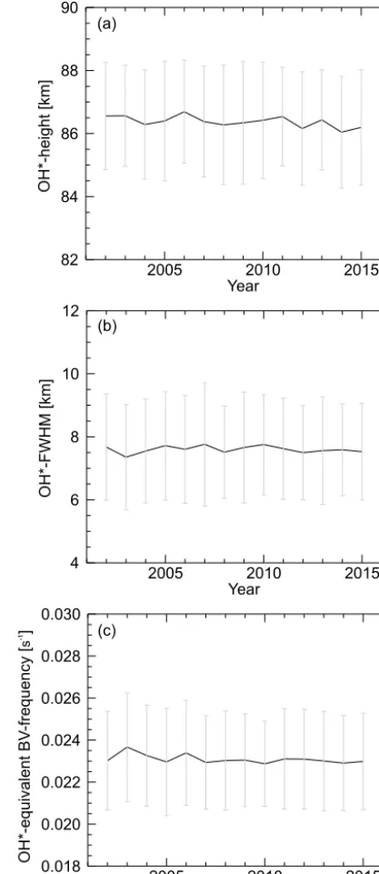
The yearly means of the three parameters, OH* layer height, FWHM, and OH*-equivalent BV frequency, show nearly no variations for the years 2002–2015 (black line in Fig. 1a– c). They reach ca. 86.5 and 7.5 km for the OH* layer height and the FWHM, and 0.023 s−1 for the OH*-equivalent BV frequency.
However, the yearly means of these parameters are accom-panied by varying standard deviations (grey bars in Fig. 1a– c), which range between approximately 2 % for the OH* layer height, 10 % for the OH*-equivalent Brunt–Väisälä fre-quency, and 20–30 % for the FWHM. They are due to char-acteristic intra-annual variations of the parameters.
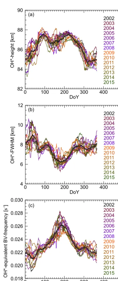
The yearly course of the OH* layer height averaged over the years 2002–2015 varies between ca. 85 and 87.5 km (thick line in Fig. 2a). The minimum is reached for the days of the year (DoY) 1–10 (January) and 320–366 (November– December), the maximum around DoY 90 and 220 (March– April and August). The mean FWHM has a minimum be-tween 6 and 6.5 km around DoY 180, and maxima at 9, 8, and 8 km approximately for DoY 40 (February), 110 (April), and 285 (October), respectively (thick line in Fig. 2b). The mean OH*-equivalent BV frequency ranges between 0.021 s−1 for DoY 40 (February) and 0.026 s−1 for DoY 185 (July), approximately (Fig. 2c, thick line). The coloured lines in Fig. 2a–c refer to the individual years and show 30-point run-ning means.
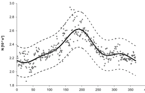
So, one can say the following: the intra-annual variabil-ity dominates the inter-annual one by far. This provides the possibility of giving an analytic description for the OH*-equivalent BV frequency, which is identical for every year. The yearly course of the BV frequency is dominated by a minimum at the beginning of the year and a maximum in the middle of the year looking quite symmetric (see Fig. 2c), which suggests the use of a spectral analysis. Therefore, we apply harmonic analysis (all-step approach) to the daily mean data (diamonds in Fig. 3). The harmonic analysis provides amplitude, phase, and period of the oscillations which ex-plain the data variability best (see Bittner et al., 1994, or Wüst and Bittner, 2006, for further information about the method). When searching for three oscillations, the annual, semi-annual, and ter-annual mode are found (information about amplitude and phases are given in Table 1). The an-nual mode dominates the other two modes by a factor of 2–3. The semi-annual and the ter-annual mode are approx-imately of the same amplitude. The superposition of these three sinusoidals (solid line in Fig. 3) explains ca. 74 % of the data variability. The data deviate 16 % at maximum from
2005 2010 2015
Year 82
84 86 88 90
OH*-height [km]
2005 2010 2015
Year 4
6 8 10 12
OH*-FWHM [km]
2005 2010 2015
Year 0.018
0.020 0.022 0.024 0.026 0.028 0.030
OH*-equivalent BV
-frequency [
]
s
-1
(a)
(b)
(c)
Figure 1.The yearly means of the height of the maximal OH-VER (denoted as OH* height, see a), the FWHM (b), and the OH*-equivalent BV frequency(c)are nearly constant from 2002 to 2015 (black curve) but show comparatively large standard devia-tions (grey bars) for each year.
oscil-Table 1. Period, amplitude, and phase of the three oscilla-tions which explain the variability of the daily OH*-equivalent BV frequency values (averaged over all years) best. They os-cillate around a constant value of 2.32×10⁻²s−1. The OH*-equivalent BV frequency [s−1] can be estimated by 2.32×10⁻²+
3 P
i=1 Aisin
2π
Ti ·DoY−ϕi
. Due to leap years, the total number of
days for one year is set to 366, which means 1 March is DoY 61 for every year.
“Annual” “Semi-annual” “Ter-annual” oscillation oscillation oscillation
PeriodT[d] 364.7 182.4 121.3
AmplitudeA[10−2s−1] 0.19 0.07 0.05
Phaseϕ[rad] 1.70 −1.69 2.36
lation is probably not a geophysical period but may result in-stead from the local time sampling of the satellite or the fact that it performs a yaw manoeuvre once every 60 days (rotat-ing through 180◦) to keep SABER viewing away from the sun. Therefore, we propose to use three sinusoidals with the parameters mentioned in Table 1 to approximate the yearly course of the OH*-equivalent BV frequency with an uncer-tainty interval of±5 or±10 % to include ca. 84 or 98 % of the data.
As mentioned above, the total uncertainties for single SABER temperature profiles are about 5 K at 90 km height with systematic uncertainties of ca. 3 K. Since we calculate a mean of the OH*-equivalent BV frequency for every DoY using data of 14 years and approximate these values by a su-perposition of harmonic oscillations, we argue that we only have to pay attention to systematic uncertainties. Assuming that the systematic uncertainties change only slightly from one height step to the next one, then they mainly influence the absolute temperature value but not the temperature gradi-ent. Assuming a “true” temperature T1=200 K and a
mea-sured temperature T2=203 K, then the difference between
the “true” squared BV frequencyN12and the measured one
N22relative toN12is
N12−N22 N12
= g T1
dT dz −0
− g
T2
dT dz −0
g T1
dT dz −0
(7)
= 1 T1−
1 T2
1 T1
=T2−T1
T2
≈1.5 %.
For the (non-squared) BV frequency, the difference is ca. 0.75 %. That means an uncertainty of ca. 3 K in temperature leads to a relative uncertainty of ca. 1.5 % (0.75 %) in the (non-)squared BV frequency. This is negligible when using the superposition of the annual, semi-annual, and ter-annual mode with an uncertainty interval of ±5 or ±10 % for the approximation of the OH*-equivalent BV frequency.
2002 2003 2004 2005 2006 2007 2008 2009 2010 2011 2012 2013 2014 2015
0 100 200 300 400 500
DoY 82 84 86 88 90 OH*-height [km] 2002 2003 2004 2005 2006 2007 2008 2009 2010 2011 2012 2013 2014 2015
0 100 200 300 400 500
DoY 4 6 8 10 12 OH*-FWHM [km] 2002 2003 2004 2005 2006 2007 2008 2009 2010 2011 2012 2013 2014 2015
0 100 200 300 400 500
DoY 0.018 0.020 0.022 0.024 0.026 0.028 0.030 OH*-equivalent BV -frequency [ ] s -1 (a)
(b)
(c)
Figure 2.OH* height(a), FWHM(b), and OH*-equivalent BV fre-quency(c)show characteristic variations during the year (coloured lines: 30-point running means of the daily mean values with mir-rored edge points for the beginning of 2002 and the end of 2015). The values of the individual years deviate most from the mean over all years (black line) during winter and especially at the beginning of the year. This might be due to enhanced atmospheric dynamics which is for example represented by stratospheric warming events and its effects on the mesopause.
A larger effect is caused by the height dependence ofg, which also influences0. According to Wüst et al. (2017),gat mesopause height (in the following denoted withghd, hd for
1.8 2.0 2.2 2.4 2.6 2.8 3.0
0 50 100 150 200 250 300 350 400
N [
10
-²s -1]
DoY
Figure 3. The superposition of the annual, semi-annual, and ter-annual oscillation (solid line) explains ca. 74 % of the variability of the daily OH*-equivalent BV frequency values averaged over all years (diamonds). 97.8 % of the data are located in a±10 % interval (dashed lines) around the curve.
its surface value. Following CIRA-86, the temperature gradi-ent at the mesopause ranges between ca. 1.4 and 2.9 K km−1 (see Fig. 4). The straightforward calculation according to
N2 Nhd2
= g
ghd ·
dT dz −
g cp dT dz −
ghd
cp
(8)
shows that squared BV frequencyNhd2 is ca. 7 % lower com-pared to the case of constantg.
The dependence of the BV frequency on temperature and its vertical gradient causes the variability during the year. Due to the meridional circulation, the mesopause temper-ature is high in winter and low in summer. Since the in-verse temperature is needed for the calculation of the BV frequency, the latter becomes low in winter and high in sum-mer. This behaviour has been reported previously by Bills and Gardner (1993) and Wüst et al. (2016). Figure 5 of Wüst et al. (2016) shows the OH*-equivalent BV frequency for the years 2012/2013 above the station OHP based on TIMED-SABER and CIRA data. In contrast to the approach presented here, the OH* height and its FWHM are kept constant (86.2 and 7.9 km calculated for July 2012 to June 2013) there. Nev-ertheless, the SABER-based OH*-equivalent BV frequency is systematically higher than the one based on CIRA (0.019– 0.022 s−1) regardless of the calculation method employed here or in Wüst et al. (2016).
The OH*-emission height (and in some instances the FWHM of the OH* layer) was already investigated on a case study basis about 30–40 years ago mostly relying on rocket-borne or lidar measurements (Good, 1976; von Zahn et al., 1987; Baker and Stair, 1988). The investigation of the OH* layer on a multi-year data basis started with the launch of WINDII (Wind Imaging Interferometer) on board UARS (Upper Atmosphere Research Satellite) in September 1991. Due to the latitudinal range of 42◦ in one hemisphere to
83 84 85 86 87 88 89 90
180 230 280 330 380 430 480 530
Hei
gh
t
[km]
Temperature, shifted [K]
January February March April May June July August September October November December
Figure 4.The temperature gradient based on CIRA-86 data for 45◦N between 83 and 90 km height is negative during the whole year. The steepest gradient is reached in March and September (ca. 20 K/7 km); it differs least from zero in summer (June–July, ca. 10 K/7 km). The temperature values are offset by+30 K per month for all months except January.
72◦in the other alternating every 36 days (e.g. Shepherd et al., 2006), publications using this data set, like for example Zhang and Shepherd (1999), focus on the tropics and low midlatitudes and are thus not suitable for a comparison with our results.
For SCIAMACHY (SCanning Imaging Absorption spec-troMeter for Atmospheric CHartographY) on board EN-VISAT (ENVironmental SATellite), von Savigny (2015) pub-lished a mean OH (3–1) emission altitude for 40–50◦N of 85.9 km (January 2003–December 2011, see his Table 3). Due to the latitudinal coverage of SCIAMACHY, these val-ues refer to September–March. For these months and the addressed latitudinal range (43.93–48.09◦N), the emission altitude of the SABER OH-B channel presented in our Fig. 2a (thick line) reaches 84.5–87.5 km and shows reason-able agreement with a mean value of ca. 86 km. In contrast to our analysis, von Savigny (2015) refers to the centroid al-titude, while we show the altitude of maximum VER. These values differ if the OH-VER profile is asymmetric. Further-more, remaining tidal effects due to different overpass times of both satellites and vertical shifts between the different Meinel bands may also play a role. So, considering these pos-sible sources of inconsistencies, the agreement is even quite good.
OH-VER profiles are also broadened when the OH-OH-VER peak descends. This fits qualitatively to the yearly development of the FWHM and OH* height (see Fig. 2a and b).
The latter seems to descend between 2002 and 2015. If one calculates the mean error of the yearly mean OH* height, which is the standard deviation (grey bars in Fig. 2a) divided by the square root of the number of data points used per year (between 509 and 590, see Sect. 2.2), the result reaches ca. 0.07 km (standard deviation of 1.5 km divided by
√ 509). In Fig. 2a, the OH* height descends ca. 0.25 km in 14 years (ca. 0.02 km year−1), which is significant within the error bars. This value lies in the same range as the ones derived by Bre-mer and Peters (2008) for low-frequency reflection heights (ca. 80–83 km) and by Teiser and von Savigny (2017) for the OH(3–1) centroid altitude based on SCIAMACHY mea-surements. Unfortunately, the SCIAMACHY results refer to latitudes between 5◦S and 30◦N; higher northern latitudes are not covered. Bremer and Peters (2008) investigated the annual means of the low-frequency reflection heights mea-sured at a constant solar angle with midpoint of the transmis-sion path at 50.71◦N and 6.61◦E between 1959 and 2006. After elimination of the solar and geomagnetically induced signal, the authors deduce a trend of−0.032 km year−1. For the development of the OH*-equivalent BV frequency, this is currently not of importance: at least between 2007 and 2015, the OH*-equivalent BV frequency stayed constant (Fig. 1c). For the integration of a possible long-term development, it is therefore too early. However, it shows that this question needs to be revisited in a couple of years.
4 Summary and outlook
We investigate the OH* layer height, FWHM, and OH*-equivalent BV frequency based on 14 years of TIMED-SABER data for 43.93–48.09◦N and 5.71–12.95◦E.
Their annual means reach ca. 86.5 km, 7.5 km, and 2.35× 10⁻²s−1and are nearly stable during 2002–2015. The char-acteristic intra-annual variations of the parameters lead to standard deviations of approximately 2 % for the OH* layer height, 10 % for the OH*-equivalent BV frequency, and 20– 30 % for the FWHM.
Since the intra-annual variability dominates the inter-annual one by far, we can provide an analytic description for the mean OH*-equivalent BV frequency, which is identical for every year. The superposition of an annual, semi-annual, and ter-annual oscillation explains ca. 74 % of the data vari-ability. Ca. 85 or 98 % of the data are located in a±5 % or ±10 % interval around the mean curve.
Similar investigations are planned for other NDMC sta-tions in order to facilitate the estimation of the nightly mean density of wave potential energy independent of co-located measurements which deliver vertical temperature profiles.
Data availability. The SABER data are available at the SABER homepage http://saber.gats-inc.com/data.php.
Competing interests. The authors declare that they have no conflict of interest.
Acknowledgements. The work of Sabine Wüst was funded by the Bavarian State Ministry for the Environment and Consumer Protec-tion (VAO project LUDWIG, project number TUS01 UFS-67093).
The article processing charges for this open-access publication were covered by a Research
Centre of the Helmholtz Association.
Edited by: Sheila Kirkwood
Reviewed by: Christian von Savigny and one anonymous referee
References
Andrews, D. G.: An introduction to atmospheric physics, Cam-bridge University Press, 2000.
Baker, D. J. and Stair Jr., A. T.: Rocket measurements of the altitude distributions of the hydroxyl airglow, Phys. Scr., 37, 611–622, 1988.
Bills, R. E. and Gardner, C. S.: Lidar observations of the mesopause region temperature structure at Urbana, J. Geophys. Res., 98, 1011–1021, https://doi.org/10.1029/92JD02167, 1993.
Bittner, M., Offermann, D., Bugaeva, I. V., Kokin, G. A., Koshelkov, J. P., Krivolutsky, A., Tarasenko, D. A., Gil-Ojeda, M., Hauchecorne, A., Lübken, F.-J., de la Morena, B. A., Mourier, A., Nakane, H., Oyama, K. I., Schmidlin, F. J., Soule, I., Thomas, L., and Tsuda, T.: Long period/large scale oscilla-tions of temperature during the DYANA campaign, J. Atmos. Terr. Phys., 56, 1675–1700, 1994.
Bremer, J. and Peters, D.: Influence of stratospheric ozone changes on long-term trends in the meso- and lower thermosphere, J. At-mos. Sol.-Terr. Phys., 70, 1473–1481, 2008.
Committee on Space Research; NASA National Space Sci-ence Data Center: COSPAR International ReferSci-ence At-mosphere (CIRA-86): Global Climatology of Atmospheric Parameters, NCAS British Atmospheric Data Centre, 7 March 2017, available at: http://catalogue.ceda.ac.uk/uuid/ 4996e5b2f53ce0b1f2072adadaeda262, 2006.
Garcia, F. J., Taylor, M. J., and Kelley, M. C.: Two-dimensional spectral analysis of mesospheric airglow image data, Appl. Opt., 36, 7374–7358, 1997.
Good, R. E.: Determination of atomic oxygen density from rocket borne measurement of hydroxyl airglow, Planet. Space Sci., 24, 389–395, 1976.
Hannawald, P., Schmidt, C., Wüst, S., and Bittner, M.: A fast SWIR imager for observations of transient features in OH airglow, At-mos. Meas. Tech., 9, 1461–1472, https://doi.org/10.5194/amt-9-1461-2016, 2016.
cyclones and cold fronts, J. Atmos. Sol.-Terr. Phys. 128, 8–23, https://doi.org/10.1016/j.jastp.2015.03.001, 2015.
Liu, G. and Shepherd, G. G.: An empirical model for the altitude of the OH nightglow emission, Geophys. Res. Lett., 33, L09805, https://doi.org/10.1029/2005GL025297, 2006.
López-Puertas, M., Garcia-Comas, M., Funke, B., Picard, R. H., Winick, J. R., Wintersteiner, P. P., Mlynczak, M. G., Mertens, C. J., Russell III, J. M., and Gordley, L. L.: Evidence for an OH (v) excitation mechanism of CO24.3 µm nighttime emission from SABER/TIMED measurements, J. Geophys. Res., 109, D09307, https://doi.org/10.1029/2003JD004383, 2004.
Lu, X., Liu, A. Z., Swenson, G. R., Li, T., Leblanc, T., and McDer-mid, I. S.: Gravity wave propagation and dissipation from the stratosphere to the lower thermosphere, J. Geophys. Res., 114, D11101, https://doi.org/10.1029/2008JD010112, 2009. Lu, X., Chu, X., Fong, W., Chen, C., Yu, Z., Roberts, B.
R., and McDonald, A. J.: Vertical evolution of potential en-ergy density and vertical wave number spectrum of Antarc-tic gravity waves from 35 to 105 km at McMurdo (77.8◦ S, 166.7◦E), J. Geophys. Res.-Atmos., 120, 2719–2737, https://doi.org/10.1002/2014JD022751, 2015.
Mertens, C. J., Schmidlin, F. J., Goldberg, R. A., Remsberg, E. E., Pesnell, W. D., Russell III, J. M., Mlynczak, M. G., López-Puertas, M., Wintersteiner, P. P., Picard, R. H., Winick, J. R., and Gordley, L. L.: SABER observations of mesospheric tempera-tures and comparisons with falling sphere measurements taken during the 2002 summer MaCWAVE campaign, Geophys. Res. Lett., 31, L03105, https://doi.org/10.1029/2003GL018605, 2004. Mertens, C. J., Fernandez, J. R., Xu, X., Evans, D. S., Mlynczak, M. G., and Russell III, J. M.: A new source of auroral infrared emission observed by TIMED/SABER, Geophys. Res. Lett., 35, 17–20, 2008.
Mlynczak, M. G.: Energetics of the mesosphere and lower thermo-sphere and the SABER experiment, Adv. Space Res. 20, 1177– 1183, https://doi.org/10.1016/S0273-1177(97)00769-2, 1997. Mulligan, F. J., Dyrland, M. E., Sigernes, F., and Deehr, C.
S.: Inferring hydroxyl layer peak heights from ground-based measurements of OH(6-2) band integrated emission rate at Longyearbyen (78◦N, 16◦E), Ann. Geophys., 27, 4197–4205, https://doi.org/10.5194/angeo-27-4197-2009, 2009.
Mzé, N., Hauchecorne, A., Keckhut, P., and Thétis, M.: Vertical distribution of gravity wave potential energy from long-term Rayleigh lidar data at a northern mid-dle latitude site, J. Geophys. Res., 119, 12069–12083, https://doi.org/10.1002/2014JD022035, 2014.
Noll, S., Kausch, W., Kimeswenger, S., Unterguggenberger, S., and Jones, A. M.: Comparison of VLT/X-shooter OH and O2 rota-tional temperatures with consideration of TIMED/SABER emis-sion and temperature profiles, Atmos. Chem. Phys., 16, 5021– 5042, https://doi.org/10.5194/acp-16-5021-2016, 2016. Pautet, P.-D., Taylor, M., Pendleton, W., Zhao, Y., Yuan, T., Esplin,
R., and McLain, D.: Advanced mesospheric temperature map-per for high-latitude airglow studies, Appl. Opt., 53, 5934–5943, 2014.
Placke, M., Hoffmann, P., Gerding, M., Becker, E., and Rapp, M.: Testing linear gravity wave theory with simultaneous wind and temperature data from the mesosphere, J. Atmos. Sol.-Terr. Phys. 93, 57–69, https://doi.org/10.1016/j.jastp.2012.11.012, 2013.
Rauthe, M., Gerding, M., and Lübken, F.-J.: Seasonal changes in gravity wave activity measured by lidars at mid-latitudes, J. At-mos. Chem. Phys., 8, 13741–13773, https://doi.org/10.5194/acp-8-6775-2008, 2008.
Remsberg, E. E., Marshall, B. T., Garcia-Comas, M., Krueger, D., Lingenfelser, G. S., Martin-Torres, J., Mlynczak, M. G., Russell III, J. M., Smith, A. K., Zhao, Y., Brown, C., Gordley, L. L., Lopez-Gonzalez, M. J., Lopez-Puertas, M., She, C.-Y., Taylor, M. J., and Thompson, R. E.: Assessment of the quality of the Ver-sion 1.07 temperature versus pressure profiles of the middle at-mosphere from TIMED/SABER, J. Geophys. Res., 113, D17101, https://doi.org/10.1029/2008JD010013, 2008.
Russell III, J. M., Mlynczak, M. G., Gordley, L. L., Tansock Jr., J. J., and Esplin, R. W.: Overview of the SABER experiment and preliminary calibration results, Proc. SPIE 3756, Optical Spectroscopic Tech. Instrum, Atmos. Space Res. III, 277–288, https://doi.org/10.1117/12.366382, 1999.
Sedlak, R., Hannawald, P., Schmidt, C., Wüst, S., and Bittner, M.: High-resolution observations of small-scale gravity waves and turbulence features in the OH airglow layer, Atmos. Meas. Tech., 9, 5955–5963, https://doi.org/10.5194/amt-9-5955-2016, 2016. She, C. Y., Yu, J. R., Huang, J. W., Nagasawa, C., and
Gard-ner, C. S.: Na temperature lidar measurements of grav-ity wave perturbations of wind, densgrav-ity and temperature in the mesopause region, Geophys. Res. Lett., 18, 1329–1331, https://doi.org/10.1029/91GL01517, 1991.
Shepherd, G. G., Cho, Y.-M., Liu, G., Shepherd, M. G., and Roble, R. G.: Airglow variability in the context of the global meso-spheric circulation, J. Atmos. Sol.-Terr. Phys., 68, 2000–2011, https://doi.org/10.1016/j.jastp.2006.06.006, 2006.
Teiser G. and von Savigny, C.: Variability of OH(3-1) and OH(6-2) emission altitude and volume emission rate from 2003 to 2011, J. Atmos. Sol.-Terr. Phys., 161, 28–42, 2017.
Tsuda, T., Nishida, M., Rocken, C. H., and Ware, R. H.: A global morphology of gravity wave activity in the stratosphere revealed by the GPS occultation data (GPS/MET), J. Geophys. Res., 105, 7257–7273, https://doi.org/10.1029/1999JD901005, 2000. von Savigny, C.: Variability of OH(3-1) emission altitude from 2003
to 2011: Long-term stability and universality of the emission rate-altitude relationship, J. Atmos. Sol.-Terr. Phys., 127, 120– 128, https://doi.org/10.1016/j.jastp.2015.02.001, 2015.
von Savigny, C., McDade, I. C., Eichmann, K.-U., and Bur-rows, J. P.: On the dependence of the OH* Meinel emis-sion altitude on vibrational level: SCIAMACHY observations and model simulations, Atmos. Chem. Phys., 12, 8813–8828, https://doi.org/10.5194/acp-12-8813-2012, 2012.
von Zahn, U., Fricke, K. H., Gerndt, R., and Blix, T.: Mesospheric temperatures and the OH layer height as derived from ground-based lidar and OH* spectrometry, J. Atmos. Terr. Phys., 49, 863–869, 1987.
Wachter, P., Schmidt, C., Wüst, S., and Bittner, M.: Spatial grav-ity wave characteristics obtained from multiple OH(3-1) airglow temperature time series, J. Atmos. Sol.-Terr. Phys., 135, 192– 201, https://doi.org/10.1016/j.jastp.2015.11.008, 2015
Wüst, S. and Bittner, M.: Non-linear resonant wave-wave interac-tion (triad): Case studies based on rocket data and first appli-cation to satellite data, J. Atmos. Sol.-Terr. Phys., 68, 959–976, https://doi.org/10.1016/j.jastp.2005.11.011, 2006.
Wüst, S., Wendt, V., Schmidt, C., Lichtenstern, S., Bittner, M., Yee, J.-H., Mlynczak, M. G., and Russell III, J. M.: Derivation of gravity wave potential energy density from NDMC measurements, J. Atmos. Sol.-Terr. Phys., 138, 32–46, https://doi.org/10.1016/j.jastp.2015.12.003, 2016.
Wüst, S., Schmidt, C., Bittner, M., Price, C., Silber, I., Yee, J.-H., Mlynczak, M. G., and Russell III, J. M.: First ground-based observations of mesopause temperatures above the Eastern-Mediterranean Part II: OH*-climatology and grav-ity wave activgrav-ity, J. Atmos. Sol.-Terr. Phys., 155, 104–111, https://doi.org/10.1016/j.jastp.2017.01.003, 2017.