* Corresponding author
E-mail: [email protected] (M. Granada-Echeverri)
2019 Growing Science Ltd. doi: 10.5267/j.ijiec.2018.6.003
International Journal of Industrial Engineering Computations 10 (2019) 295–308
Contents lists available at GrowingScience
International Journal of Industrial Engineering Computations
homepage: www.GrowingScience.com/ijiec
A mixed integer linear programming formulation for the vehicle routing problem with backhauls
Mauricio Granada-Echeverria*, Eliana M. Torob and Jhon Jairo Santac
aProgram of Electrical Engineering, Universidad Tecnológica de Pereira, Pereira, Colombia
bFaculty of Industrial Engineering, Universidad Tecnológica de Pereira, Pereira, Colombia
cProgram of Physical Engineering, Universidad Tecnológica de Pereira and Universidad Libre Seccional Pereira
C H R O N I C L E A B S T R A C T
Article history: Received March 9 2018 Received in Revised Format March 16 2018
Accepted June 14 2018 Available online June 14 2018
The separate delivery and collection services of goods through different routes is an issue of current interest for some transportation companies by the need to avoid the reorganization of the loads inside the vehicles, to reduce the return of the vehicles with empty load and to give greater priority to the delivery customers. In the vehicle routing problem with backhauls (VRPB), the customers are partitioned into two subsets: linehaul (delivery) and backhaul (pickup) customers. Additionally, a precedence constraint is established: the backhaul customers in a route should be visited after all the linehaul customers. The VRPB is presented in the literature as an extension of the capacitated vehicle routing problem and is NP-hard in the strong sense. In this paper, we propose a mixed integer linear programming formulation for the VRPB, based on the generalization of the open vehicle routing problem; that eliminates the possibility of generating solutions formed by subtours using a set of new constraints focused on obtaining valid solutions formed by Hamiltonian paths and connected by tie-arcs. The proposed formulation is a general-purpose model in the sense that it does not deserve specifically tailored algorithmic approaches for their effective solution. The computational results show that the proposed compact formulation is competitive against state-of-the-art exact methods for VRPB instances from the literature.
© 2019by the authors; licensee Growing Science, Canada Keywords:
Arborescence Backhaul
Integer linear programming Linehaul
Vehicle routing problem
1. Introduction
inside the vehicles at each delivery point. The pickups and deliveries of goods in a mixed order, or simultaneously, cause difficulties due to the rearrangements of goods on board. The VRPB adequately represents this strategic need and must satisfy the following conditions:
Each vertex must be visited exactly once by a single route. That is, each vertex is grade 2. Each route starts and _nishes at the depot.
Each customer must be fully attended when visited. All customers are serviced from a single depot.
The vehicle capacity should never be exceeded in both the linehaul and backhaul route and all vehicles have the same capacity.
In each circuit the linehaul vertices precede the backhaul vertices, if any. That is:
o A circuit of only BCs is not allowed.
o The last customer of a linehaul route is always connected with the depot or with BC who is starting a backhaul route.
o The last BC of a backhaul route is always connected with the depot.
o The precedence constraint is also justi_ed by the need to attend to LCs with higher priority than BCs.
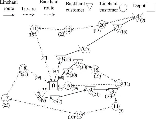
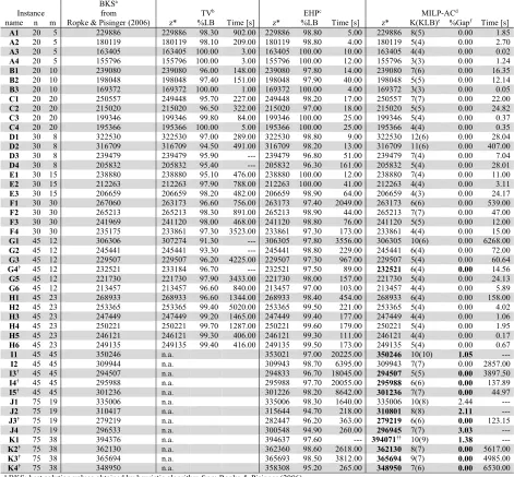
Fig. 1 shows the optimal solution of a VRPB example with 20 customers; in which the first 10 customers are LCs and the other 10 are BCs. For this case, the capacity of all vehicles is the same and equal to Q = 60. The minimum number of vehicles needed to serve all the linehaul and backhaul customers is known in advance and is indicated by KL and KB, respectively. These values can be obtained by solving the bin-packing problem instances associated with the corresponding customer subset, which calls for the determination of the minimum number of bins, each with capacity Q, needed to serve all customers (Toth & Vigo, 2002). To ensure feasibility, we assume that the number of vehicles needed K must be greater than or equal to the maximum value between KL and KB, i.e., K = max {KL, KB}. Thus, in this example, the minimum number of vehicles needed to serve all the linehaul and backhaul customers is KL=KB = 3.
Linehaul route
Backhaul
route Backhaul customer
Tie-arc Linehaul customer Depot
7
(16)4
(9) 20(15)
5
(7) 12(23)
10 (15)
[47] 11
(19)
[57]
0
2
(30)[60]
6
(30) 15 (19)
13(11) 16(29)
[59]
8
(9)
[53]
1
(7)9
(21) (16)
3
14 (5) 19
(10) (23)
17
18 (21)
[59]
M. Granada-Echeverri et al.
The demands of each customer are shown in the figure with the notation (·), and the incoming and outgoing flow of goods at each depot are shown with the notation [·]. The depot is denoted with a rectangle, the LCs with triangles, and the BCs with circles. Table 1 shows the coordinates of all vertices and their respective demands.
Because the VRPB is NP-hard in the strong sense, it can be solved as a matching problem (Toth & Vigo, 2002); it has two types of routes and has a precedence constraint, so many heuristic processes are appropriate and efficient for the solution. Therefore, most existing literatures on the VRPB are related to heuristics and metaheuristics methodologies with high quality results. A comprehensive review of metaheuristic techniques for VRPB is found in Ropke and Pisinger (2006). Two literature reviews cover the main works about VRPB: the first, presented by Toth and Vigo (2002), presents the existing work up to 2002 and second, by Irnich et al. (2014a,b), focuses on complementing the review up to 2013.
Table 1
Coordinates and loads for 20 customers
X coord. Y coord. Demand
0 25 32 0
1 25 25 7
Produ
ct to
be d
eliv
er
ed
2 30 40 30
3 50 30 16
4 60 70 9
5 37 52 7
6 35 45 30
7 52 64 16
8 20 26 9
9 40 30 21
10 28 47 15
11 17 63 19
Produ
ct
to
be co
llected
12 31 62 23
13 52 33 11
14 51 21 5
15 42 41 19
16 31 32 29
17 5 25 23
18 12 42 21
19 36 16 10
20 45 65 15
Concerning the exact approaches, few jobs have been proposed (Toth & Vigo, 2014). In our review, only two works were found: the first exact method is reported by Toth and Vigo (1997), in which an effective Lagrangian bound is introduced that extends the methods previously proposed for the capacitated VRP (CVRP). The resulting Branch-and-Bound algorithm is able to solve problems with up to 70 customers in total. The second exact method is proposed by Mingozzi et al. (1999), in which a set-partitioning-based approach is presented and the resulting mixed integer linear programming (MIP) is solved through a complex procedure. The results show that the approach is capable of solving undirected problems with up to 70 customers. Toth and Vigo state that no exact approaches have been proposed for VRPB during the last decade (Toth & Vigo, 2014). In our review, we have reached the same conclusion and new proposals for unified exact models of VRPB were not found, since the only two existing proposals are used to derive the relaxations on which the exact approaches are based (Toth & Vigo, 1997).
very different; direct comparisons between the problems serving pickups and deliveries in a mixed order or simultaneously with problems that deliver first and pick-up second should not be performed, since they are addressing different requirements. The VRPB is a problem with a special structure of the routes that consist of two distinct parts; a delivery and a pickup segment. A complete review of these two types of problems can be found in Ropke and Pisinger (2006), Wade and Salhi (2003) and Parragh et al. (2008).
More recently, Chávez et al. (2016) proposed a Pareto ant colony algorithm to solve a multi-objective variant of the multidepot VRPB where the aim is to minimize distance, travel time and energy consumption. A random fixed speed between 30 km/h and 90 km/h was assigned to each arc, and the function considered by Bektaş and Laporte (2011) was used to compute energy consumption. The algorithm is based on the idea of Doerner et al. (2004) which uses three matrices of pheromones for each objective function. The method was tested on new instances based on those of Salhi and Nagy (1999). In Chávez et al. (2018) a heuristic algorithm based on Tabu Search Approach for solving the VRPB is proposed. The proposed algorithm considers intensification of local information and the proper exploitation of local search procedures combined with exploratory stochastic strategies. The solution strategy considers the design of separate routes for both delivery and collection of goods.
A metaheuristic algorithm based on the ant colony optimization was presented by Chávez et al. (2015), to solve the multi-depot vehicle routing problem with delivery and collection of package. Each performed route consists of one sub-route in which only the delivery task is done, in addition to one sub-route in which only the collection process is performed. The proposed algorithm tries to find the best order to visit the customers at each performed route.
A recent survey paper with interesting conclusions and research perspectives on the VRPB, including models, exact and heuristic algorithms, variants, industrial applications and case studies, are identified in Koç and Laporte (2017). In this review, the authors highlight the importance of using matheuristic algorithms that allow the interoperation of metaheuristic and mathematical programming techniques. Additionally, they identify the need for new studies focused on developing effective and powerful exact methods to solve all available standard VRPB instances to optimality. The authors also conclude that no electric vehicle version has yet been studied for the VRPB.
In VRPB the precedence constraint, which stipulates that in each circuit the linehaul vertices precede the backhaul vertices, difficult to build an exact model from the traditional viewpoint of the CVRP. This is because traditional restrictions for the elimination of sub-tours perfectly fit into VRPs with a unique set of vertices, where the evaluation of constraints of degree or conservation of flow can be evaluated in a general way on all vertices. Adapting these restrictions to the VRPB involves special cases such as vertices at the end of a linehaul route, vertices at the start of a backhaul route and routes with linehaul customers only.
M. Granada-Echeverri et al.
In practice, the OVRP formulation represents situations such as: home delivery of packages and newspapers, school bus routing, routing of coal mines material, and the shipment of hazardous materials (Braekers et al., 2015). Thus, the VRPB structure can be seen as OVRPs of linehaul and backhaul routes connected by tie-arcs. The proposed model is a general-purpose model in the sense that it does not deserve specifically tailored algorithmic approaches for their effective solution and can be solved by an integer-programming solver. The main contributions of this paper can be summarized as follows:
A unified and compact model for the VRPB is proposed, which can be a starting point for the generalization of problems shortly discussed in the literature, as are the multi-depot VRPB and the location VRPB.
This paper presents a contribution to the discussion on VRPB and its feature from a new approach based on arborescence, which allows the best advantage of the structure of the problem. The proposed model can be used to derive new relaxations on which the exact approaches are based. The proposed formulation allows to solve the symmetric and asymmetric VRPB and it is able to
minimize the number of used vehicles.
The rest of the paper is organized as follows: in Section 2 we first describe the problem formulation, presenting the nomenclature for the variables and parameters used in the mathematical model. We then introduce the new mixed integer linear programming (MILP) formulations based on the arborescence condition (MILP-AC) for the VRPB. We describe how the arborescence constraints operate on the different structures of the problem. In Section 3 we present a computational study performed on 142 test instances. Finally, the conclusions in Section 4 are presented.
2. Problem formulation
2.1. Nomenclature
The nomenclature for the variables and parameters of the proposed model for the VRPB is summarized next.
Sets:
L Set of linehaul customers. L = {1,...,n}.
B Set of backhaul customers. B = {n + 1,...,n + m}.
L0 Set of linehaul customers and the depot, L0 = {0} ∪L. Vertex 0 corresponds to the depot. B0 Set of backhaul customers and the depot, B0 = {0} ∪B.
CU Set of linehaul and backhaul customers, CU = L ∪B.
V Parameters:
Set of nodes V = {0} ∪CU.
Cij Cost of traveling between nodes I and j.
Dj Nonnegative quantity of product to be delivered or collected (demand) of the customer j
∈CU.
KL, KB Minimum number of vehicles needed to serve all the linehaul and backhaul customers,
respectively.
Q Capacity of the vehicles (identical vehicles).
Variables:
sij Binary variable for the use of the path between nodes i, j ∈V.
ξij Binary variable for the use of the path between nodes i ∈L and j ∈B0 ( tie-arcs ).
2.1. The VRP with Backhauls
Note that in the optimal solution shown in Fig. 1 the linehaul routes, excluding the tie-arcs, constitute a subproblem that has a radial configuration (arborescence) starting from the depot, spanning all the linehaul vertices and ending up at a client. This subproblem we have named linehaul open vehicle routing problem (LOVRP). Similarly, the backhaul routes also have a radial configuration, entering the depot and spanning all the backhaul vertices; this sub-problem is named backhaul open vehicle routing problem (BOVRP). Thus, the arborescence characteristics allow to handle the VRPB as the solution of two open routing subproblems (ORPs) connected through a tie-arc. In the OVRP context, the necessary condition for obtaining a minimum spanning tree is that the number of arcs be equal to the number of customer nodes, which is given by the cardinality of the sets L and B for the case of the LOVRP and BOVRP, respectively. However, this condition is necessary but not sufficient because two situations can be presented: i) there may be customer nodes with a degree greater than two and ii) disconnected solutions can be obtained. To avoid the first situation, it must be considered that a spanning tree becomes a sub-graph formed only by Hamiltonian paths if each customer node has a degree less than or equal to two. Concerning the second situation, the addition of a balance condition of the demand flow by each customer node avoids getting disconnected solutions. These situations are considered in the model presented below.
2.3. Proposed Model for the VRPB
The two-index vehicle flow formulation for the VRPB is defined as follows:
∈
∈ ∈∈
(1)
S.t.
∈ ∈
| | (2)
∈ ∈
∀ ∈ (3)
∈ 1
∀ ∈ (4)
∈ ∈ ∈
∀ ∈ (5)
⋅ ∀ ∈ ∀ ∈ (6)
∈
∈ , (7)
∈ ∈
| | (8)
∈ ∈
∀ ∈ (9)
∈ 1
∀ ∈ (10)
∈ ∈ ∈
M. Granada-Echeverri et al.
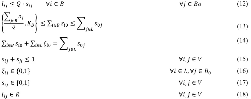
⋅ ∀ ∈ ∀ ∈ (12)
∈ , ∑
∈
∈ (13)
∑∈ ∑∈
∈
(14)
1 ∀ , ∈ (15)
∈ 0,1 ∀ ∈ , ∀ ∈ (16)
∈ 0,1 ∀ , ∈ (17)
∈ ∀ , ∈ (18)
The objective function (1) minimizes operating costs, which correspond to the sum of the total travelling cost of the routes used to deliver and collect the goods to the customers and the total travelling cost associated with use of the tie-arcs connecting the last customer of a linehaul route with the first customer of a backhaul route or with the depot. The set of constraints (2)-(7) model the LOVRP, where (2) and (3) impose the arborescent connectivity requirements. More precisely, these two constraints allow configuring one shortest spanning arborescence linehaul with fixed indegree KL at the depot vertex. In the optimal solution of the LOVRP, each route has an arborescent configuration formed by a minimum spanning tree; starting from the depot, spanning all the nodes, and ending at a customer. A comprehensive discussion on the application of concepts of graph theory for the formulation of spanning tree constraints is found in works related to optimizing the operation of distribution systems (DS) of electric power, which has been an active topic for years, with recent emphasis on smart grid initiatives. Distribution systems are most commonly operated in radial configurations in order to keep the system operation as simple as possible. In this context, a radial configuration is equivalent to a spanning tree, where there is only one path between the electrical substation and final consumers. The resulting subgraph must be connected, without cycles and with a number of arcs that is equal to the number of demand nodes. A brief review of existing approaches for imposing spanning tree constraints in the operation of the DS, can be found in Ahmadi and Martí (2015). Thus, several of the concepts of graph theory used in DS can be used in the LOVRP since both problems are quite similar.
(a) Constraint (2). (b) Constraints (2), (4) and (5). (c) Constraints (2)-(5).
Fig. 2. Impact of the spanning tree constraints in the LOVRP subgraph
the outdegree constraints (5) impose that exactly one arc leaves each customer, except for those customers who are at the end of the route where the tie-arcs emerging from LC to a BC or to the depot should be considered. However, the addition of these degree constraints in directed graphs may not represent a spanning tree, because a disconnected graph can be obtained, as shown in Fig. 2(b). The addition of flow balance constraint by each customer node avoids getting disconnected solutions, since an infeasible solution is obtained when the goods leaving the depot can not reach the customers. Thus, the set of constraints reported in (3) guarantees network connectivity through the balance of the demand flow by each customer so that they are fully served when visited, and also ensures that the remaining demand of a vehicle is zero after the vehicle has serviced its last customer. The impact of these constraints is shown in Figure 2(c), where the demands of each customer are shown with the notation (∙) and the amount of goods owing through the arcs are shown with the notation [∙]. Thus, the constraints (2)-(5) allow obtaining a linehaul arborescence structure as shown in Fig. 2(c), whose main characteristic is that each vertex is of degree 2 when tie-arcs are considered. Constraint (6) and (7) impose both the vehicle and depot capacity requirements, respectively, associated with the linehaul routes only. The first is an upper limit defined by the capacity of the vehicle to transport a given quantity of product on any linehaul-arc, while the second is a lower limit to the number of routes out of the depot to supply linehaul customers, which is determined by the ratio between the total demand to be collected and the vehicle capacity. Constraint (7) limits the minimum number of vehicles used on linehaul routes. When there is a choice of set partitioning or set covering as a formulation, set covering is preferred (Barnhart et al. 1998).
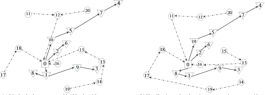
(a) Linehaul arborescence and backhaul antirborescence. (b) Hamiltonian paths when degree constraints are considered. Fig. 3. Arborescence paths for 20 customers example
Similarly, the set of constraints (8) - (13) model the BOVRP, were (8) and (9) impose the antiarborescent connectivity requirements. Note that (9) guarantees the balance of demand flow in each BC, so that the product is fully collected when the customer is visited. Out-degree constraint (10) imposes that exactly one arc leave each vertex associated with a BC. In Figure 3(a), an example of the shortest spanning arborescence linehaul, with fixed indegree KL at the depot vertex, is shown in solid lines. Similarly, the
shortest spanning antiarborescence backhaul, with fixed indegree KB at the depot vertex, is shown in
dashed lines. In Figure 3(b), in solid lines, the impact of constraints (2)-(5) is shown, allowing generating a linehaul arborescence structure. In dashed lines, the impact of constraints (8)-(10) is shown, allowing generating a backhaul antiarborescence structure.
M. Granada-Echeverri et al.
problems (LOVRP and BOVRP) through the tie-arcs and to ensure the characteristic of precedence. Because the symmetric and asymmetric versions of VRPB are considered, the uni-directional constraint (15) ensures that only one of the two variables sij or sji must be used. Finally, constraints (16) and (17)
define all binary decision variables, and constraint (18) defines the real variable.
Table 2
Computational results for the VRPB cases from Goetschalckx and Jacobs-Blecha (1989), the Euclidean distances were rounded to one decimal and the final result was rounded to an integer
BKSa
Instance from TVb EHPc MILP-ACd
name n m Ropke & Pisinger (2006) z* %LB Time [s] z* %LB Time [s] z* K(KLB)e %Gapf Time [s]
A1 20 5 229886 229886 98.30 902.00 229886 98.80 5.00 229886 8(5) 0.00 1.85
A2 20 5 180119 180119 98.10 209.00 180119 98.80 4.00 180119 5(4) 0.00 2.70
A3 20 5 163405 163405 100.00 3.00 163405 100.00 10.00 163405 4(4) 0.00 0.02
A4 20 5 155796 155796 100.00 3.00 155796 100.00 12.00 155796 3(3) 0.00 1.24
B1 20 10 239080 239080 96.00 148.00 239080 97.80 14.00 239080 7(6) 0.00 16.35
B2 20 10 198048 198048 97.40 151.00 198048 97.90 40.00 198048 5(5) 0.00 12.14
B3 20 10 169372 169372 100.00 1.00 169372 100.00 4.00 169372 3(3) 0.00 0.05
C1 20 20 250557 249448 95.70 227.00 249448 98.20 17.00 250557 7(7) 0.00 22.00
C2 20 20 215020 215020 96.50 322.00 215020 97.00 18.00 215020 5(5) 0.00 24.82
C3 20 20 199346 199346 99.80 84.00 199346 100.00 25.00 199346 5(4) 0.00 0.37
C4 20 20 195366 195366 100.00 5.00 195366 100.00 25.00 195366 4(4) 0.00 0.35
D1 30 8 322530 322530 97.00 289.00 322530 98.80 9.00 322530 12(6) 0.00 28.04
D2 30 8 316709 316709 94.50 491.00 316709 98.20 13.00 316709 11(6) 0.00 407.00
D3 30 8 239479 239479 95.90 --- 239479 96.80 51.00 239479 7(4) 0.00 7.04
D4 30 8 205832 205832 95.40 --- 205832 96.30 161.00 205832 5(4) 0.00 28.01
E1 30 15 238880 238880 95.10 476.00 238880 100.00 12.00 238880 7(4) 0.00 11.00
E2 30 15 212263 212263 97.90 788.00 212263 100.00 41.00 212263 4(4) 0.00 3.11
E3 30 15 206659 206659 98.20 482.00 206659 98.90 64.00 206659 4(3) 0.00 24.17
F1 30 30 267060 263173 96.60 756.00 263173 97.40 2049.00 263173 6(6) 0.00 539.00
F2 30 30 265213 265213 98.30 891.00 265213 98.90 44.00 265213 7(7) 0.00 47.00
F3 30 30 241969 241120 98.00 468.00 241120 98.80 76.00 241120 5(5) 0.00 12.00
F4 30 30 235175 233861 97.30 3523.00 233861 97.30 173.00 233861 4(4) 0.00 15.00
G1 45 12 306306 307274 91.30 --- 306305 97.80 3556.00 306305 10(6) 0.00 6268.00
G2 45 12 245441 245441 93.30 --- 245441 98.80 229.00 245441 6(4) 0.00 72.00
G3 45 12 229507 229507 96.20 4225.00 229507 97.30 967.00 229507 5(4) 0.00 60.64
G4† 45 12 232521 233184 96.70 --- 232521 97.50 89.00 232521 6(4) 0.00 14.56
G5 45 12 221730 221730 97.90 3433.00 221730 98.00 157.00 221730 5(4) 0.00 24.13
G6 45 12 213457 213457 96.60 840.00 213457 97.00 103.00 213457 4(4) 0.00 5.89
H1 45 23 268933 268933 96.60 1344.00 268933 98.40 454.00 268933 6(4) 0.00 158.00
H2 45 23 253365 253365 99.40 5020.00 253365 99.50 221.00 253365 5(4) 0.00 4.02
H3 45 23 247449 247449 99.20 1465.00 247449 99.40 177.00 247449 4(4) 0.00 1.06
H4 45 23 250221 250221 99.70 1287.00 250221 99.60 179.00 250221 5(4) 0.00 1.95
H5 45 23 246121 246121 99.30 406.00 246121 99.30 111.00 246121 4(4) 0.00 0.17
H6 45 23 249135 249135 99.40 416.00 249135 99.50 173.00 249135 5(4) 0.00 0.67
I1 45 45 350246 n.a. 353021 97.00 20225.00 350246 10(10) 1.05 ---
I2 45 45 309944 n.a. 309943 98.70 6395.00 309943 7(7) 0.00 2857.00
I3† 45 45 294507 n.a. 294833 96.70 18045.00 294507 5(5) 0.00 3897.50
I4† 45 45 295988 n.a. 295988 97.70 20055.00 295988 6(6) 0.00 137.89
I5† 45 45 301236 n.a. 301226 98.20 8642.00 301236 7(7) 0.00 44.97
J1 75 19 335006 n.a. 335006 98.30 1640.00 335006 10(8) 2.44 ---
J2 75 19 310417 n.a. 315644 94.70 218.00 310801 8(8) 2.11 ---
J3† 75 19 279219 n.a. 282447 96.20 363.00 279219 6(6) 0.00 123.15
J4 75 19 296533 n.a. 300548 94.90 260.00 296945 7(7) 3.03 ---
K1 75 38 394376 n.a. 394637 97.60 --- 394071†† 10(9) 1.38 ---
K2† 75 38 362130 n.a. 362360 98.60 2618.00 362130 8(7) 0.00 5617.00
K3† 75 38 365694 n.a. 365693 98.50 3812.00 365694 9(7) 0.00 4985.00
K4† 75 38 348950 n.a. 358308 95.20 265.00 348950 7(6) 0.00 6530.00
a BKS: best solution values obtained by heuristic algorithm from Ropke & Pisinger (2006).
b TV: exact algorithm proposed by Toth & Vigo (1997). Computing times in Pentium 60 MHz. Time limit of 6,000 seconds. c EHP: exact algorithm proposed by Mingozzi et al. (1999). Computing times in SGI 200 MHz. Time limit of 25,000 seconds.
d MILP-AC: proposed mixed integer linear programming with radility condition formulation. Computing times in PC intel i3/3.3 GHz. Time limit of
6600 seconds.
e K(KLB): K is the specified number (given in advance) of vehicles to use and KLB is the number of vehicles performing routes conformed by linehaul
and backhaul customers. Thus, K − KLB is the number of vehicles performing routes conformed by linehaul customers exclusively. z*: value of the best solution found by the earlier algorithms.
LB(%): percentage error of the lower bound (LB) computed at the root node. It is calculated as the ratio of the LB divided by the best z* and multiplied by 100.
f Gap (%): percentage gap is calculated as (CPLEX − LB)/LB.
†: optimality proven for the first time. ††: new BKS.
Time: overall computing time expressed in CPU seconds.
To reduce the number of binaries and to speed up computational time we apply the preconditioning valid constraints (19), (20) and (21) to remove unfeasible arcs.
∈ ∈
0 (19)
∈
0 (20)
∈ ∈
0 (21)
The constraint (19) guarantees that there is no connection from one BC to a LC. The beginning of a route cannot be through a BC, because a route consisting exclusively of BCs is not allowed, which is ensured through (20). Finally, constraint (21) ensures that the tie-arcs linking a LCi with a BCj or with the depot
should only be handled by the variable ξij.
3. Computational results for the exact algorithms
Two datasets of scenarios are used in order to show the operation and effectiveness of the proposed formulation. The first dataset, denoted as GJ dataset, was proposed by Goetschalckx & Jacobs-Blecha (1989) and contains 62 instances with a range between 20 and 150 customers. Details on how these scenarios were generated can be consulted in Toth & Vigo (2002). The second dataset, denoted as TV dataset, was proposed by Toth & Vigo (1997) and contains 33 instances between 21 and 100 customers. The proposed model corresponds to a MIP formulation and were implemented in AMPL (Fourer et al., 2002) and solved with GUROBI 6.5 (called with the optimality gap option equal to 0%), on an Intel Core i3 computer; 3.3 GHz, 3.8 GB of RAM.
In Tables 2 and 3, the results for the VRPB using the GJ and TV datasets, respectively, are compared with those obtained by exact methods proposed by Toth and Vigo (1997) and Mingozzi et al. (1999). Additionally, the best-known solutions (BKS) reported by the heuristic method proposed by Ropke & Pisinger (2006) is presented in the fourth column of each table, which are the state of the art of heuristic methods for VRPB instances from the literature. In Table 2, we give in columns 1-3: the problem name, the number of LCs and the number of BCs, respectively. Column 4 presents the BKS obtained by a heuristic procedure (Ropke & Pisinger, 2006). In columns 5-7 and 8-10 the results are presented for TV and EHP algorithms, respectively.
For each of these algorithms the table reports two types of information: i) the value of the best solution found by the algorithm, z*, and ii) the overall computing time expressed in CPU seconds. The Euclidean distances were rounded to one decimal and the final result was rounded to an integer. Finally in columns 9-12 the characteristics of the solution for each problem are presented, using the proposed formulation in this paper (computing times in PC Intel i3/3.3 GHz and time limit of 6600 seconds).
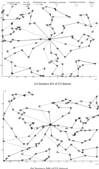
The optimality for the GJ dataset was proved for the first time for 8 instances. One new best-known solutions was found considering both heuristic methods and exact methods and 12 new BKS were found in the tests considering a comparison between exact methods only. Optimality was achieved in 42 of the 47 scenarios. As an example, in Figure 3a the optimal solution for the instance K4 is shown.
M. Granada-Echeverri et al.
Table 3
Computational results for the VRPB cases from Toth & Vigo (1997)
BKSa
Instance from TVb EHPc MILP-ACd
name n m Ropke & Pisinger (2006) z* %LB Time [s] z* %LB Time [s] z* K(KLB)e %Gapf Time [s]
EIL2250A 11 10 371 371 100.00 3.00 371 100.00 6.00 371 3(3) 0.00 0.01
EIL2266A 14 7 366 366 100.00 6.00 366 100.00 3.00 366 3(3) 0.00 0.01
EIL2280A 17 4 375 375 98.90 55.00 375 99.20 6.00 375 3(3) 0.00 0.01
EIL2350A 11 11 682 682 100.00 2.00 682 100.00 1.00 682 2(2) 0.00 0.01
EIL2366A 15 7 649 649 98.80 65.00 649 99.40 7.00 649 2(2) 0.00 0.01
EIL2380A 18 4 623 623 98.10 36.00 623 98.70 9.00 623 2(2) 0.00 0.01
EIL3050A 15 14 501 501 100.00 3.00 501 100.00 8.00 501 2(2) 0.00 0.01
EIL3066A 20 9 537 537 98.50 119.00 537 97.60 17.00 537 3(3) 0.00 0.30
EIL3080A 24 5 514 514 100.00 13.00 514 97.90 31.00 514 3(3) 0.00 0.30
EIL3350A 16 16 738 738 98.40 292.00 738 100.00 46.00 738 3(2) 0.00 0.14
EIL3366A 22 10 750 750 94.80 1338.00 750 100.00 27.00 750 3(2) 0.00 0.38
EIL3380A 26 6 736 736 93.90 1655.00 736 99.30 44.00 736 3(3) 0.00 7.31
EIL5150A 25 25 559 559 99.30 441.00 559 99.60 66.00 559 3(3) 0.00 1.80
EIL5166A 34 16 548 548 97.80 2754.00 548 99.30 68.00 548 4(4) 0.00 2.01
EIL5180A 40 10 565 565 98.00 4436.00 565 98.10 691.00 565 4(3) 0.00 26.11
EILA7650A 37 38 739 739 98.20 15931.00 739 99.20 884.00 739 6(6) 0.00 64.21
EILA7666A 50 25 768 768 95.40 13464.00 768 99.00 1205.00 768 7(6) 0.00 743.00
EILA7680A 60 15 781 781 90.50 --- 781 97.70 596.00 781 8(5) 0.99 ---
EILB7650A 37 38 801 801 97.60 16345.00 801 99.30 124.00 801 8(7) 0.00 40.96
EILB7666A 50 25 873 873 91.20 12990.00 873 99.00 2918.00 873 10(8) 0.94 ---
EILB7680A 60 15 919 919 85.20 10414.00 919 99.50 821.00 933 12(6) 3.92 ---
EILC7650A 37 38 713 713 98.90 10343.00 713 98.90 16659.00 713 5(5) 0.00 8.64
EILC7666A 50 25 734 734 97.60 --- 734 99.20 952.00 734 6(6) 0.00 185.00
EILC7680A 60 15 733 733 93.70 --- 733 97.80 --- 733 7(5) 1.50 ---
EILD7650A 37 38 690 690 99.70 401.00 690 99.70 197.00 690 4(4) 0.00 6.03
EILD7666A† 50 25 715 715 98.50 --- 715 98.60 5023.00 715 5(5) 0.00 32.54
EILD7680A† 60 15 694 703 96.80 --- 694 99.00 20148.00 694 6(4) 0.00 845.00
EILA10150A† 50 50 831 843 96.30 --- 843 96.30 364.00 831 4(4) 0.00 938.00
EILA10166A 67 33 846 846 99.20 10913.00 846 99.60 434.00 846 6(6) 0.00 6.00
EILA10180A 80 20 857 916 9.30 --- 908 91.70 431.00 859 7(6) 0.82 ---
EILB10150A† 50 50 925 n.a. 933 95.60 --- 923†† 7(7) 0.00 792.00
EILB10166A 67 33 989 n.a. 1056 89.10 293.00 971†† 10(8) 2.99 --- EILB10180A 80 20 1008 n.a. 1022 97.20 20199.00 1013 11(9) 1.46 --- The nomenclature of this table is the same as that presented in Table 2.
Time limits were 18000, 25000 and 1000 seconds for methods TV, EHP and MILP-AC, respectively.
Table 4
Examples of results minimizing the number of vehicles
Instance MILP-AC (number of vehicles given in advance) MILP-AC (number of vehicles given in advance)
name n z*m K(KLB)e Time %Gapf z*[s] K(KLB)e Time %Gapf [s]
C3 20 20 199346 5(4) 0.00 0.37 195367 4(4) 0.00 2.06
G4 1245 232521 6(4) 0.00 14.56 229507 5(4) 0.00 111.00
G5 45 12 221730 5(4) 0.00 24.13 218485 4(4) 0.00 77.00
conditions and this can be exploited in future works using heuristics techniques or to formulate new relaxations in exact approaches based in branch-and-bound techniques. For example, the solution of the BOVRP, which is simpler than the LOVRP under the above conditions, could be an interesting starting point for a more elaborate methodology. As can be seen from the computational results, the proposed model produces high quality results, obtaining equal or better upper bounds in all instances, and the final lower bounds prove stronger than those obtained by earlier methods.
Fig. 3. Examples of VRPB optimal solutions
0.2 0.4 0.6 0.8 1 1.2 1.4 1.6 1.8 2 2.2
x 104
0.5 1 1.5 2 2.5
x 104
0 1 2 3 4 5 6 7 8 9 10 11 12 13 14 15 16 17 18 19 20 21 22 23 24 25 26 27 28 29 30 31 32 33 34 35 36 37 38 39 40 41 42 43 44 45 46 47 48 49 50 51 52 53 54 55 56 57 58 59 60 61 62 63 64 65 66 67 68 69 70 71 72 73 74 75 76 77 78 79 80 81 82 83 84 85 86 87 88 89 90 91 92 93 94 95 96 97 98 99 100 101 102 103 104 105 106 107 108 109 110 111 112 113 114 115 116 117 118 119 120 121 122 123 124 125
(b) Instance M4 of GJ dataset
0.2 0.4 0.6 0.8 1 1.2 1.4 1.6 1.8 2 2.2
x 104
0.5 1 1.5 2 2.5
x 104
0 1 2 3 4 5 6 7 8 9 10 11 12 13 14 15 16 17 18 19 20 21 22 23 24 25 26 27 28 29 30 31 32 33 34 35 36 37 38 39 40 41 42 43 44 45 46 47 48 49 50 51 52 53 54 55 56 57 58 59 60 61 62 63 64 65 66 67 68 69 70 71 72 73 74 75 76 77 78 79 80 81 82 83 84 85 86 87 88 89 90 91 92 93 94 95 96 97 98 99 100 101 102 103 104 105 106 107 108 109 110 111 112 113
M. Granada-Echeverri et al.
Table 5
Computational results for the VRPB cases from Goetschalckx & Jacobs-Blecha (1989) with the Euclidean distances rounded to integers
Instance Heuristic algorithm MILP-AC (number of vehicles given in advance)
name n m BKSa Referenceb z* K(KLB)e %Gapf Time [s]
A1 20 5 229884 TV 229884 8(5) 0.00 6.01
A2 20 5 180117 TV 180117 5(4) 0.00 1.43
A3 20 5 163403 TV 163403 4(4) 0.00 0.56
A4 20 5 155795 TV 155795 3(3) 0.00 0.03
B1 20 10 239077 TV 239077 7(6) 0.00 3.33
B2 20 10 198045 TV 198045 5(5) 0.00 0.74
B3 20 10 169368 TV 169368 3(3) 0.00 0.01
C1 20 20 250557 TV 250557 7(7) 0.00 22.39
C2 20 20 215019 TV 215019 5(5) 0.00 11.00
C3 20 20 199344 TV 199344 5(4) 0.00 0.41
C4 20 20 195365 TV 195365 4(4) 0.00 0.67
D1 30 8 322533 TV 322533 12(6) 0.00 16.33
D2 30 8 316711 TV 316711 11(6) 0.00 405.03
D3 30 8 239482 TV 239482 7(4) 0.00 57.44
D4 30 8 205834 TV 205834 5(4) 0.00 95.00
E1 30 15 238880 TV 238880 7(4) 0.00 16.63
E2 30 15 212262 TV 212262 4(4) 0.00 5.43
E3 30 15 206658 TV 206658 4(3) 0.00 2.85
F1 30 30 263175 TV 263175 6(6) 0.00 485.00
F2 30 30 265214 TV 265214 7(7) 0.00 32.35
F3 30 30 241121 OW 241121 5(5) 0.00 15.41
F4 30 30 233861 TV 233861 4(4) 0.00 11.27
G1 45 12 306304 OW 306304 10(6) 0.53
---G2 45 12 245441 TV 245441 6(4) 0.00 53.73
G3 45 12 229506 OW 229506 5(4) 0.00 14.58
G4 45 12 232519 LNS 232519 6(4) 0.00 42.49
G5 45 12 221731 OW 221731 5(4) 0.00 19.44
G6 45 12 213457 TV 213457 4(4) 0.00 2.61
H1 45 23 268933 OW 268933 6(4) 0.00 396.00
H2 45 23 253366 TV 253366 5(4) 0.00 3.81
H3 45 23 247449 TV 247449 4(4) 0.00 2.22
H4 45 23 250221 TV 250221 5(4) 0.00 2.09
H5 45 23 246121 TV 246121 4(4) 0.00 1.64
H6 45 23 249136 TV 249136 5(4) 0.00 1.22
I1 45 45 350248 LNS 350248 10(10) 0.00 12911.00
I2 45 45 309946 LNS 309946 7(7) 0.00 794.00
I3 45 45 294509 OW 294509 5(5) 0.00 1539.00
I4 45 45 295988 TV 295988 6(6) 0.00 64.58
I5 45 45 301238 LNS 301238 7(7) 0.00 43.73
J1 75 19 335004 LNS 335478 10(8) 1.84
---J2 75 19 310417 LNS 311969 8(8) 2.25
---J3 75 19 279220 LNS 279220 6(6) 0.00 77.00
J4 75 19 296533 LNS 297088 7(6) 2.84
---K1 75 38 394369 LNS 394068†† 10(9) 1.41
---K2 75 38 362128 LNS 362128 8(7) 0.00 3925.00
K3 75 38 365693 LNS 365693 9(7) 0.00 4520.00
K4 75 38 348947 LNS 348947 7(6) 0.00 3210.00
L1 75 75 426014 LNS 426014 10(10) 3.90
---L2 75 75 401231 LNS 401231 8(8) 1.60
---L3 75 75 402681 LNS 402681 9(9) 1.30
---L4 75 75 384635 LNS 384635 7(7) 0.00 12834.00
L5 75 75 387563 LNS 387563 8(7) 0.00 4479.00
M1 100 25 400085 LNS 403267 11(7) 4.65
---M2 100 25 397448 LNS 398430 10(8) 3.23
---M3 100 25 377093 LNS 377429 9(8) 3.49
---M4 100 25 348530 LNS 348138†† 7(6) 0.00 11077.00
N1 100 50 408921 OW 408097†† 11(10) 0.34
---N2 100 50 409275 OW 408062†† 10(10) 0.71
---N3 100 50 396162 OW 394334†† 9(9) 0.94
---N4 100 50 394785 LNS 394,785 10(9) 0.97
---N5 100 50 373471 LNS 373,471 7(7) 0.00 5774.00
N6 100 50 373752 LNS 373,752 8(7) 0.00 4749.00
aBKS: best solution values obtained by heuristic algorithm and reported in Ropke & Pisinger (2006).
bReference: the heuristic algorithm reporting the result is indicated in this column. TV refers to the heuristic algorithm by Toth & Vigo (1999), OW refers to
the heuristic by Osman & Wassan (2002) and LNS refers to the heuristic by Ropke & Pisinger (2006).
†† : new BKS.
References
Barnhart, C., Boland, N. L., Clarke, L. W., Johnson, E. L., Nemhauser, G. L., & Shenoi, R. G. (1998). Flight
string models for aircraft fleeting and routing. Transportation Science, 32(3), 208-220.
Bektaş, T., & Laporte, G. (2011). The pollution-routing problem. Transportation Research Part B:
Bodin, L. D., Golden, B. L., Assad, A., & Ball, M. 0.(1983) Routing and scheduling of vehicles and crews:
The state of the art. Computers and Operations Research, 10, 63-21.
Braekers, K., Ramaekers, K., & Van Nieuwenhuyse, I. (2016). The vehicle routing problem: State of the art
classification and review. Computers & Industrial Engineering, 99, 300-313.
Chávez, J., Escobar, J., & Echeverri, M. (2016). A multi-objective Pareto ant colony algorithm for the
Multi-Depot Vehicle Routing problem with Backhauls. International Journal of Industrial Engineering
Computations, 7(1), 35-48.
Chávez, J., Escobar, J., Echeverri, M., & Meneses, C. (2018). A heuristic algorithm based on tabu search for
vehicle routing problems with backhauls. Decision Science Letters, 7(2), 171-180.
Doerner, K., Gutjahr, W. J., Hartl, R. F., Strauss, C., & Stummer, C. (2004). Pareto ant colony optimization:
A metaheuristic approach to multiobjective portfolio selection. Annals of Operations Research, 131(1-4),
79-99.
Fourer, R., Gay, D. M., & Kernighan, B. W. (1990). A modeling language for mathematical
programming. Management Science, 36(5), 519-554.
Goetschalckx, M., & Jacobs-Blecha, C. (1989). The vehicle routing problem with backhauls. European
Journal of Operational Research, 42(1), 39-51.
Irnich, S., Schneider, M., & Vigo, D. (2014a). Chapter 9: Four Variants of the Vehicle Routing Problem.
In Vehicle Routing: Problems, Methods, and Applications, Second Edition (pp. 241-271). Society for
Industrial and Applied Mathematics.
Irnich, S., Toth, P., & Vigo, D. (2014b). Chapter 1: The family of vehicle routing problems. In Vehicle
Routing: Problems, Methods, and Applications, Second Edition (pp. 1-33). Society for Industrial and Applied Mathematics.
Koç, Ç., & Laporte, G. (2017). Vehicle Routing with Backhauls: Review and Research
Perspectives. Computers & Operations Research.
Mingozzi, A., Giorgi, S., & Baldacci, R. (1999). An exact method for the vehicle routing problem with
backhauls. Transportation Science, 33(3), 315-329
Osman, I. H., & Wassan, N. A. (2002). A reactive tabu search meta‐heuristic for the vehicle routing problem
with back‐hauls. Journal of Scheduling, 5(4), 263-285.
Parragh, S. N., Doerner, K. F., & Hartl, R. F. (2008). A survey on pickup and delivery problems. Journal für
Betriebswirtschaft, 58(1), 21-51
Ropke, S., & Pisinger, D. (2006). A unified heuristic for a large class of vehicle routing problems with
backhauls. European Journal of Operational Research, 171(3), 750-775.
Santa Chávez, J. J., Echeverri, M. G., Escobar, J. W., & Meneses, C. A. P. (2015). A Metaheuristic ACO to
Solve the Multi-Depot Vehicle Routing Problem with Backhauls. International Journal of Industrial
Engineering and Management (IJIEM), 6(2), 49-58.
Salhi, S., & Nagy, G. (1999). A cluster insertion heuristic for single and multiple depot vehicle routing
problems with backhauling. Journal of the operational Research Society, 50(10), 1034-1042.
Schrage, L. (1981). Formulation and structure of more complex/realistic routing and scheduling
problems. Networks, 11(2), 229-232.
Toth, P., & Vigo, D. (1997). An exact algorithm for the vehicle routing problem with
backhauls. Transportation Science, 31(4), 372-385.
Toth, P., & Vigo, D. (1999). A heuristic algorithm for the symmetric and asymmetric vehicle routing problems
with backhauls. European Journal of Operational Research, 113(3), 528-543.
Toth, P., & Vigo, D. (Eds.). (2002). The vehicle routing problem. Society for Industrial and Applied
Mathematics.
Wade, A., & Salhi, S. (2003). An ant system algorithm for the mixed vehicle routing problem with backhauls. In Metaheuristics: computer decision-making (pp. 699-719). Springer, Boston, MA.