Performance Analysis of Mixed Logit Models for Discrete Choice Models

for Discrete Choice Models

Jaka Nugraha

Department of Statistics

Universitas Islam Indonesia, Indonesia jnugraha@uii.ac.id

Abstract

Mixed Logit model (MXL) is generated from Multinomial Logit model (MNL) for discrete, i.e. nominal, data. It eliminates its limitations particularly on estimating the correlation among responses. In the MNL, the probability equations are presented in the closed form and it is contrary with in the MXL. Consequently, the calculation of the probability value of each alternative get simpler in the MNL, meanwhile it needs the numerical methods for estimation in the MXL. In this study, we investigated the performance of maximum likelihood estimation (MLE) in the MXL and MNL into two cases, the low and high correlation circumstances among responses. The performance is measured based on differencing actual and estimation value. The simulation study and real cases show that the MXL model is more accurate than the MNL model. This model can estimates the correlation among response as well. The study concludes that the MXL model is suggested to be used if there is a high correlation among responses.

Keywords: Logit; Maximum Likelihood; Monte Carlo simulation; Utility model

Introduction

Discrete choice models (DCM) describe decision maker’s choices among alternatives. The decision makers can be people, households, firms, or any other decision-making unit, and the alternatives might represent competing products, courses of action, or any other options or items over which choices must be made. Multinomial Probit Model (MNP), MNL and Mixed Logit Model (MXL) are part of DCM. These models are often used to analyze the discrete choices made by individuals recorded in survey data. These models have been applied in marketing, transportation, political research, energy, housing etc. (Camminatiello and Lucadamo, 2010; Yang, 2010; Lovreglio et al., 2016; Merkert and Beck, 2017).

Each model has advantages and disadvantages. The advantage of MNL is to have a simpler form of equation in estimating the model. The weakness of MNL is that the model is prepared by using irrelevant alternative independence (IIA). Meanwhile, MNP was developed to overcome MNL weakness in terms of IIA. However MNP has an open form of equation, so its model estimation requires simulation and iteration methods such as Newton-Raphson.

procedure to represent the distribution of the random parameter model (Train, 2016). However it raises the next issue on how accurate the MXL compared to MNL.

This paper, the profile of MXL for detecting the correlation among alternatives on utilities models is studied. Model was constructed and applied for simulation data on several rank of dependency (correlation) among alternatives and R.3.1.1 software was adopted to run the computational work. Parameters in MXL and MNL are estimated by using the MLE method which has good properties for large samples, especially asymptotically efficient and asymptotic bias in simulated maximum likelihood estimation (Lee, 1995; Horowitz, and Savin, 2001; Lee, 1992). Based on these properties, the estimator accuracy can be measured by using the distance between the estimator and of the parameters at various levels of correlation.

Aim of study is to evaluate the effect of correlation among choice on MXL and MNL models. In order to organize the scheme of study, the specification of MNL and MXL, how to perform parameter estimation using MLE and accuracy of parameters estimation in the MNL and MXL using simulation data are presented. Some examples of the application of MNL and MXL in real cases are also described.

Utility Model

To fit in a discrete choice framework, the set of alternatives, called the choice set, needs to exhibit three characteristics. First, the alternatives must be mutually exclusive from the decision maker’s perspective. The decision maker chooses only one alternative from the choice set. Second, the choice set must be exhaustive, in that all possible alternatives are included. The decision maker necessarily chooses one of the alternatives. Third, the number of alternatives must be finite. A decision maker (respondent), denoted as i was faced with a choice among J alternatives. The respondent has a certain level utility (or profit) for each alternative j. Uij for j=1,...,J is the utility that respondent i obtain from

alternative j and the real value of Uij that is unkonwn by researcher. The decision maker

chooses the alternative that provides the greatest utility. Researcher did not know the value of utility for respondents in each option and looked at the attributes, is denoted Zij, that

exist for each choice and respondents attribute is denoted Xi.

A function that relates these observed factors to the decision maker’s utility is denoted Vij

and is often called representative utility,

𝑉_𝑖𝑗 = 𝛼_𝑗+ 𝛽_𝑗𝑋_𝑗 + 𝛾_𝑗𝑍_𝑖𝑗 (1)

where i=1,...,n and j=1,...,J. Vij is assigned as representative utility. Equation (1) is a model

constructed and reported by Boulduc (1999). Due to the unkown value of Uij , therefore

𝑈𝑖𝑗 = 𝑉𝑖𝑗 + 𝜀𝑖𝑗 . (2)

𝜺_𝑖 = (𝜀_𝑖1, … , 𝜀_𝑖𝐽)′ is a random variable having density of 𝑓(𝜺_𝑖), where Vij is observed factor and 𝜀_𝑖𝑗 is unobserved factor in utility. The density 𝑓(𝜺_𝑖) is the distribution of the unobserved portion of utility within the population of people who face the same observed portion of utility. Different choice models are derived under different specifications of the density of unobserved factors, 𝑓(𝜺𝑖).

Multinomial Logit Model (MNL)

MNL model is derived under the assumption that 𝜀𝑖𝑗 is independent and identically

𝑓(𝜀_𝑖𝑗) = exp(−𝜀_𝑖𝑗) . exp (−exp (−𝜀_𝑖𝑗) . (3) Mean and the variance from this distribution are 0.5772 and 𝜋2/6, respectively. Cummulative distribution of Extreme Value type I is

𝐹(𝜀_𝑖𝑗) = exp (−exp (−𝜀_𝑖𝑗) . (4)

The Extreme Value distribution and the Standard Normal distribution can be shown in Figure 1.

Figure 1: Extreme Value and Standard Normal distribution

Based on Figure 1, it can be seen that the Extreme Value distribution is almost symmetrical distribution with a standard normal distribution. Though this distribution has a thicker or heavy tail compared to the normal distribution. The probability of decision maker i choice k alternative is stated as:

𝜋𝑖𝑘 =_∑ exp (𝑉_{exp (𝑉}𝑖𝑘) 𝑖𝑗) 𝐽

𝑗=1

. (5)

This formula is assigned as logit probability (Train, 1998). Parameters (𝛼_𝑗, 𝛽_𝑗, 𝛾) can be estimated by using MLE.

Mixed Logit Model (MXL)

Mixed logit assumes that the unobserved portions of utility are a mixture of an independent and identically distributed (iid) extreme value term and another multivariate distribution selected by the researcher. This general specification allows MXL to avoid imposing the IIA property on the choice probabilities. Further, MXL is a flexible tool for examining heterogeneity in responden behavior through random coefficients specifications. Mixed Logit is a very flexible model that can be approached by several random utility models (McFadden and Train, 2000). In Equation (2), if a 𝛿_𝑗 random variable having density 𝑓(𝛿_𝑗) is added then utility model can served in the following form:

𝑈_𝑖𝑗 = 𝑉_𝑖𝑗 + 𝛿_𝑗+ 𝜀_𝑖𝑗. (6)

Generally, the assumption of 𝑓(𝛿𝑗) in standard normal distribution is used, 𝛿𝑗~𝑁(0,1) and 𝜹 = (𝛿₁, … , 𝛿₁)~𝑁(𝟎,).

It is assumed that 𝜀𝑖𝑗 has an extreme value distribution and is independent to 𝛿𝑗. The MXL

is a standard integral Logit in respect to density 𝜹. The probabily of i-th respondent chooses the k-th alternative can be formulated into:

where 𝑔_𝑖𝑘(𝜹)is logit probability that can be writen as:

𝑔𝑖𝑘(𝜹) =_∑ exp (𝑉_{exp (𝑉}𝑖𝑘+𝛿𝑘) 𝑖𝑗+𝛿𝑖𝑗) 𝐽

𝑗=1

(8)

The probability in MXL is a weighted mean to the logit by using weighting density function

𝑓(𝜹). The MXL is a mixed form of logit function and density function 𝑓(𝜹) and the value of probability in Equation (8) can be approached/computed by using simulation. The steps of simulation are as following (Train, 2003) :

a. Take a value of 𝜹 from density 𝑓(𝜹) and label it as 𝛿(𝑟). At the first take r=1. b. Calculate the logit probability 𝑔_𝑖𝑘(𝛿(𝑟)) from equation (8).

c. Repeate the steps 1 and 2 for R–times and evaluate the average 𝜋̃_𝑖𝑘 =_𝑅1∑𝑅 𝑔_𝑖𝑘(𝛿(𝑟)₎

𝑟=1 (9)

Maximum Likelihood Estimation (MLE) on Multinomial Distribution Let Y1,Y2,...,Yn be random variables having pooled density:

𝑓(𝒚|𝜽) = 𝑓(𝑦1, … , 𝑦𝑛|𝜃1, … , 𝜃𝐽) (10)

These functions depend on parameters 𝜽 = (𝜃1, … , 𝜃𝐽). As Yi is independent each other,

then we have

𝑓(𝒚|𝜽) =



(  (11)

The Likelihood function, labeled 𝐿(𝜽|𝒚), is a function of the parameters of a statistical model given data, is

𝐿(𝜽|𝒚) =



( (12)

Suppose  that is a probable/possible set of values for vector parameter 𝜽 and is also assigned as parameter space. In another experiment. it was defined that MLE for 𝜽, denoted as 𝜽̂_𝑀𝐿𝐸 is value of 𝜽 which maximizes the likelihood function 𝐿(𝜽|𝒚) on data y

(Greene, 2005).

𝜽̂𝑀𝐿𝐸 = argmaxL(;y)

 (13)

If Y1, Y2,...,Yn are random samples having multinomial density, then 𝑓(𝑦_𝑖|𝜋₁, … , 𝜋_𝐽) = 𝜋₁𝑦𝑖1_{… 𝜋}

𝐽 𝑦𝑖𝐽

for i=1,...,n.

The 𝜋_𝑖𝑗 is the probability of the i-th decision maker choose the j-th alternative as in the equations (5) and (7) that obtained parameter 𝜽. Therefore, 𝜋𝑖𝑗 = 𝜋𝑖𝑗(𝜽).The Likelihood

function for parameter 𝜽 can be constructed as:

𝐿(𝜽) = ∏ 𝜋_𝑖1𝑦𝑖1_{… 𝜋}

𝑖𝐽 𝑦𝑖𝐽 𝑛

𝑖=1

The log-likelihood function is

𝑙𝑜𝑔 𝐿(𝜽) =





1 1 1

i( ) log[ ]

log   (14)

MLE is the value of 𝜽 that maximizes the log 𝐿(𝜽) function or

In MXL model, 𝜋_𝑖𝑗 is a double integral that can be calculated/computed by using/implementing the simulation method. For example 𝜋̃_𝑖𝑗 is the value of 𝜋_𝑖𝑗 that was calculated by using the simulation in Equation (9). The simulated likelihood function was obtained by subtituting the 𝜋_𝑖𝑗 value into log-likehood function in Equation (14) by simulating the 𝜋̃_𝑖𝑗 value.

𝑠𝑖𝑚𝑙𝑜𝑔 𝐿(𝜽) =





1 1 1

] ~ log[ )

(

simlog  

The 𝜽̂_𝑀𝑆𝐿 is the 𝜽 value which maximizes the 𝑠𝑖𝑚𝑙𝑜𝑔 𝐿(𝜽).

𝜽̂_𝑀𝑆𝐿 =



  (15)

Simulation Studies

In order to detect the influence of correlation among alternatives, the multinomial data was generated for J=3. Three alternatives were chosen as representative for the correlation structure among alternatives for J case in general. First, there is a correlation between alternative j and j’, meanwhile there is no correlation among them. Therefore, conclusion from the simulation at case J=3 can be generalized for all value of J. It is assumed that there is a correlation among the first and the second, but there is no correlation for the third alternative.

For example an application in the selection of the mode of transport, there are three alternatives: private car, taxi, and public transport. Taxi is probably related to the private car, in a sense that for someone has no private car then taxi will be chosen and vice versa. Furthermore, the simulated data is generated using the following utility model:

𝑈𝑖1 = 𝑉𝑖1+ 𝛿𝑖1+ 𝜀𝑖1;𝑈𝑖2 = 𝑉𝑖2+ 𝛿𝑖2+ 𝜀𝑖2;𝑈𝑖3 = 𝑉𝑖3+ 𝜀𝑖3 (16)

where 𝜀_𝑖𝑗~Extreme Value type I, 𝛿_𝑖1~𝑁(0,1),𝛿_𝑖2~𝑁(0,1),𝜹 = (𝛿₁, 𝛿₂)~𝑁(𝟎,)i=1,...,n;

j=1,2,3 and = _

     1 1 12 12   .

It is assumed that 𝑉_𝑖𝑗 = 𝛼_𝑗+ 𝛽_𝑗𝑋_𝑗+ 𝛾𝑍_𝑖𝑗.Xi is a characteristic individual/decision maker

and Zij is the attribute of the alternative. Third alternative was assumed as a baseline, 𝛼3 = 𝛽3 = 0. Data was generated on parameter 𝛼1 = −1 , 𝛼2 = 1, 𝛽1 = 0.5, 𝛽2 = −0.5,𝛾 = 1 and on several value of 𝜎₁₂. Based on these simulation data was estimated by using MNL and MXL. Furthermore, based on several values of 𝜎12, estimators obtained on MXL are

compared to those were obtained by MNL. Results and Discussion

It is clear from Equation (3) that 𝑉𝑎𝑟(𝜀_𝑖𝑗) = 𝜋2/6 and is assumed that 𝜀_𝑖𝑗 and 𝛿_𝑖𝑗 are independent. Therefore, the covariance among alternatives on Equation (16) is

𝐶𝑜𝑣(𝑈𝑖) =                 + + 6 0 0 0 6 0 6 2 2 12 12 12 2 12        (17)

𝜌 = 𝐶𝑜𝑟(𝑈𝑖1, 𝑈𝑖2) = 0

6

2

12

12 

+

 

and 𝜎₁₂ =

) , ( 1

6 ). , (

2 1

2

2 1

i i

i i

U U Cor

U U Cor

−



(18)

The equation (18) shows a relationship between covarians (𝜎₁₂) to the correlation (𝜌) value. Data were generated on several values , and they are served in Table 1.

Table 1: Relationship between covarians (𝝈𝟏𝟐) to the correlation (𝝆) value.

No. 𝝈𝟏𝟐 𝝆 No. 𝝈𝟏𝟐 𝝆 No. 𝝈𝟏𝟐 𝝆 No. 𝝈𝟏𝟐 𝝆

1 0.1 0.06 6 2 0.55 11 7 0.81 16 12 0.88

2 0.2 0.11 7 3 0.65 12 8 0.83 17 13 0.89

3 0.3 0.15 8 4 0.71 13 9 0.85 18 14 0.89

4 0.5 0.23 9 5 0.75 14 10 0.86 19 15 0.90

5 1 0.38 10 6 0.79 15 11 0.87

Packages of R.3.1.1 software were employed to generate data and estimate the parameter. Some packages in R software are:

a. randtoolbox : to generate Halton series that can be used to calculate normal density integral,

b. micEcon : to calculate MLE on MNL model, c. mnormt : to generate multivariate normal data,

d. adapt : to evaluate maximum point from log-likelihood function on Mixed Logit model.

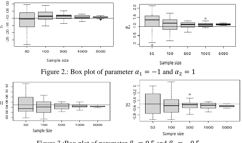
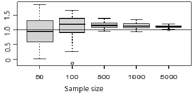
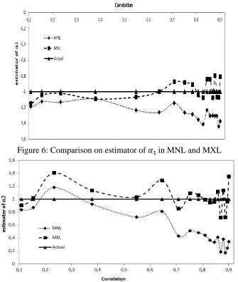
Before simulation using correlation structure as presented in Table 1, it is important to conduct simulation to observe the influence of sample size towards parameter estimation value. The observation on the effect of sample size to the estimator was conducted for the independent structure 𝜎₁₂ = 0 or 𝜌 = 0 for n=50, n=100, n=500, n=1000 and n=5000. The parameter estimation was perforemd by using geepack packages in R software. The estimation results are presented in Figure 2 – 4.

Figure 2.: Box plot of parameter 𝛼₁ = −1 and 𝛼₂ = 1

Figure 4. : Box plot of parameter 𝛾 = 1

From Figure 2-4 it is seen that for the sample size less than 100, the big variance is resulted. This is due to the wide deviation which resulted from some samples. It is concluded that for n=50 and 100 the resulted estimators are instable. Moreover, the estimator resulted from n=500, 1000 and 5000 are stable enough which there is no such wide deviation from the targeted value. The bigger sample size, the obtained estimator approaching and fit to the real values. Morever, the bigger n, the more stable estimator or the variance of each estimator is smaller.

Eventhough n is big enoughr (n=5000), the bias is still available. The reasons are, first, the generated data are in normal distribution (not from the extreme value distribution), which the normal and extreme value distribution have different variances. Mean and the variance from distribution of Extreme Value type I are 0.5772 and π2/6, respectively Generalized estimating equation (GEE) model, as utilized for geepack packages is based on the Extreme Value distribution.

Furthermore, the simulation was performed in order to evaluate the influence of towards estimator of all parameters with the sample size, n=1000. The actual correlation value and its estimation value are presented in Figure 5.

Figure 5: Plot of actual and estimate correlation

From Figure 5., it can be seen that MXL could estimate the correlation parameter, particularly on the correlation value more than 0.4. By using the hypothesis H0 :

𝜌𝑎𝑐𝑡𝑢𝑎𝑙=𝜌𝑒𝑠𝑡𝑖𝑚𝑎𝑡𝑒, it can be concluded that there is insignificant correlation among actual

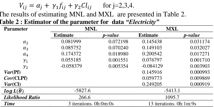
Further the bias of each parameter (𝛼₁, 𝛼₂, 𝛽₁, 𝛽₂, 𝛾) are illustrated in Figure 6 to Figure 10.

Figure 6: Comparison on estimator of 𝛼₁in MNL and MXL

Figure 7: Comparison on estimator of 𝛼₂in MNL and MXL

According to Figures 6 and 7, the 𝛼 estimator in MNL has a great bias is proportional to the magnitude of the correlation between the response. At the level of correlation is high (more than 0.7), the magnitude of the bias in 𝛼 estimator reaches more than 50%. Meanwhile, MXL is not affected by the correlation between the response. The estimators in MNL always smaller than the MXL. On the actual parameter 𝛼1 = −1, the mean of

estimator in both MNL and MXL are -1.2560 and -0.9873 respectively. By using hypothesis H0: 𝛼1 = −1, the significant difference among actual and estimated value was

observed in MNL, with the p-value of 4.011x10-9_{. Meanwhile, MXL gives the insignificant}

result among them at the p-value of 0.626.

For the actual parameter 𝛼₂ = 1, the estimator mean in MNL and MXL are 0.5578 and 1.0333 respectively. By using hypothesis H0: 𝛼₂ = 1, insignificant values of the actual

Figure 8: Comparison on estimator of 𝛽₁in MNL and MXL

Based on Figure 8, 𝛽₁ estimator in the model MNL and MXL is the same mean of 0.5488 and 0.5557 respectively. By the actual value 𝛽1 = 0.5, it can be concluded that there is

no significant difference between actual and estimated values.

On the 𝛽₂ = −0.5, the almost similar result is obtained with whose observed on the parameter , MNL gives significant difference of estimator among significant and actual values with p-value5.659x10-5_{. The mean of estimator 𝛽}

2 on MNL model is -0.3759, while

insignificant estimator among both values is observed in the MXL with p-value of 0.415. Mean of estimator 𝛽₂ on model MNL is -0.4800.

The results is in line with the parameter  that has actual value of 1 in that the MNL model produces the predictor value of 0.7347 that gives significantly difference among actual and estimated values (p-value of 3.508x10-7), meanwhile the MXL model gives the estimator value of 1.0115, insignificant difference with actual value. P-value of MXL model is 0.566.

Figure 10: Comparison on estimator of 𝛾in MNL and MXL

Figures 9 and 10 illustrate that the 𝛽₂ estimator and 𝛾 estimator in MNL have a great bias is proportional to the magnitude of the correlation between (or among) the response. Meanwhile, MXL is not affected by the correlation between (or among) the response. These results are similar to those seen in the 𝛼 parameter.

Some conclusions which can be derived from Figures 5 to 10 are: a. Correlation parameters can be well estimated by MXL.

b. In general the bias on MNL model is higher than on MXL.

c. For the intercept parameters (i.e : 𝛼₁, 𝛼₂). In case of the high correlation (more than 0.7) presents then the MNL produces a higher bias in comparison to the MXL.

d. For coefficient parameter X (i.e : 𝛽₁). bias from MNL model is relatively equal to MXL. For coefficient parameter Z (i.e : 𝛾). In case of high correlation (more than 0.5) then MNL produces a higher bias than MXL.

Applications in Real Cases

In this section, we apply the MNL and MXL in real problems. There are two cases, each represents the state of the low and high correlation circumstances. The first case represents a weak correlation is taken from data “Electricity” and the second one represents a high

correlation, is taken from the data “Heating”. Both of them are from mlogit package in

R.3.1.1

Case 1. Data “Electricity” are taken from mlogit package in R.3.1.1. A sample of residential electricity customers were asked a series of choice experiments. In each experiment, four hypothetical electricity suppliers were described. The person as asked which of the four suppliers he/she would choose (j=1,2,3,4). In the experiments, the characteristics of each supplier were stated. Pf is fixed price at a stated cents per kWh for each choice (electricity suppliers). Cl is the length of contract that the supplier offered, in years (such as 1 year or 5 years).

𝑉_𝑖𝑗 = 𝛼_𝑗+ 𝛾₁𝑓_𝑖𝑗+ 𝛾₂𝐶𝑙_𝑖𝑗 forj=2,3,4.

The results of estimating MNL and MXL are presented in Table 2.

Table 2 : Estimator of the parameter for data “Electricity”

Parameter MNL MXL

Estimate p-value Estimate p-value

𝛼2 0.081999 0.072198 0.145438 0.031174

𝛼3 0.085752 0.070240 0.149103 0.032027

𝛼4 0.174372 0.018980 0.200542 0.017271

𝛾1 0.055185 0.001551 0.076797 0.001710

𝛾2 -0.058379 0.005354 -0.084129 0.003903

Var(Pf) 0.145916 0.000993

Cov(Cl.Pf) 0.059773 0.009869

Var(Cl) 0.249205 0.000919

𝒍𝒐𝒈 𝑳(𝜽̂) -5827.6 -5413.1

Likelihood Ratio 266.6 1095.7

Time 3 iterations. 0h:0m:0s 13 iterations. 0h:1m:9s

Based on the results in Table 2, the correlation values obtained is

𝜌̂ =_{√𝑉𝑎𝑟(𝑃𝑓)𝑉𝑎𝑟(𝐶𝑙)}𝐶𝑜𝑣(𝐶𝑙.𝑃𝑓) = 0.313453

The value of this correlation still include low correlation, so that the MNL and MXL relatively the same. The calculation process in the MXL takes longer than the MNL.

The Likelihood Ratio statistic (LR) is an alternative for testing hypotheses about  defined by

𝐿𝑅 = −2𝑙𝑜𝑔𝐿(𝜃0)

𝐿(𝜃̂) (19)

where 𝜃̂ denotes the MLE of 𝜃 and 𝜃₀ denotes the restriction that H0 is true. H0 states that

all parameters 𝜽 = 𝟎. L(𝜃̂) is the value of the likelihood function at the estimated parameters dan L(0) is its value when all parameters are set equal to zero. Statistic LR is

Chi Square distributed with the degree of freedom equal to tested parameters. The value of

LR on MXL model is 1095.7 which is higher compared to that of derived by MNL model (266.6). This means that MXL model give more reliable conclusion compared with MNL model. Similar pattern is also obtained from partial test in that the p-value of MXL model is less that 0.04 while MNL model gives p-value of 𝛼₂ and 𝛼₃more are higher than 0.07 parameter.

Train (2003) reported that likelihood ratio index can be utilized for measure the fitness of model and data. The likelihood index is defined as

𝑅2 _{= 1 −} 𝐿𝑜𝑔 𝐿(𝜃̂)

𝐿𝑜𝑔 𝐿(𝜃0) (20)

R2 of MXL is 0.092 which is larger than the MNL which is 0.022. Its means that MXL model better than MNL model.

Case 2. Data “Heating” are taken from mlogit package in R.3.1.1

annual operating cost for the 5 alternatives. As type ec is stated as base line, representative utility models can be expressed as:

𝑉𝑖𝑗 = 𝛼𝑗+ 𝛾1𝐼𝑐 + 𝛾2𝑂𝑐𝑖𝑗 for j=2,3,4,5.

From 900 observations, the results of estimating MNL and MXL are presented in Table 3.

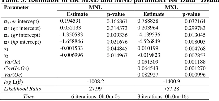
Table 3. Estimator of the MXL and MNL parameter for Data “Heating”

Parameter MNL MXL

Estimate p-value Estimate p-value

2 (er intercept) 0.194591 0.166861 0.788838 0.032164

3 (gc intercept) 0.052133 0.314373 0.203964 0.299783 4 (gr intercept) -1.350583 0.039336 -4.139536 0.013045 5 (hp intercept) -1.658846 0.021676 -4.526849 0.008003

1 -0.001533 0.044845 0.010199 0.004768

2 -0.006996 0.014967 -0.019823 0.007853

Var(Ic) 0.051509 0.001188

Cov(Ic.Oc) 0.064543 0.001270

Var(Oc) 0.082927 0.000996

log L(𝜃̂) -1008.2 -1400.9

Likelihood Ratio 27.99 757.28

Time 6 iterations. 0h:0m:0s 3 iterations. 0h:0m:16s

The correlation values obtained

𝜌̂ =_{√Var(Ic)Var(Oc)}Cov(Ic.Oc) = 0.987545

Therefore the MXL model is recommended.

The LR value on MXL model is 757.28 which is higher compared with that of derived by MNL model (27.99). It means that MXL model gives more reliable conclusion rather than the MNL model. The R2 of MXL model (0.213) is higher than the MNL model (R2=0.014) means that the MXL model is better than the MNL model. Based on these two examples, the estimator on MXL model is always higher compared to the estimator on MNL model,

|𝜃𝑀𝑋𝐿| > |𝜃𝑀𝑁𝐿|.

Conclusions

Based on data simulation, the conclusions obtained are: MXL can be used to estimate the correlation parameter properly (small bias) and MXL is better than MNL especially for alternatives of the correlation presents among alternatives. Some suggestions for further research are: a) for practitioners who will use the discrete responses in modelling and there is a correlation among alternatives, then the MXL is more appropriate than MNL. If there is no correlation among alternatives then the MNL can be used. b) Statistician can improve the computational method: where the Mixed Logit model requires a long time calculation than MNL model and other estimation methods can also be developed.

Acknowledgement

The author would like to thanks to Universitas Islam Indonesia through Hibah Percepatan Profesor, and Ministry of Research, Technology and Higher Education, Republic of Indonesia for supporting this research.

References

1. Agresti, A. (2002). Categorical Data Analysis. John Wiley & Sons.

3. Camminatiello, I. and Lucadamo, A. (2010). Estimating multinomial logit model with multicollinear data. Asian Journal of Mathematics and Statistics, 3(2), 93–100. 4. Greene W. (2005). Econometrics Analysis. 5 Editions, Prentice Hall.

5. Horowitz, J.L., and Savin, N.E. (2001). Binary response models : logits, probits and semiparametrics. Journal of Economic Perspectives, 15(4), 43–45.

6. Jain, D.C., Vilcassim, N.J., and Chintagunta, P.K. (1994). A random-coefficients logit brand-choice model applied to panel data. Journal of Business and Economic Statistics, 12(3), 317–328.

7. Lee, L. (1992). On the efficiency of methods of simulated moments and simulated likelihood estimation of discrete choice models. Econometric Theory, 8, 518–552. 8. Lee, L. (1995). Asymptotic bias in simulated maximum likelihood estimation of

discrete choice models. Econometric Theory, 11, 437–483.

9. Lovreglio, R.A., Fonzone, A.B., and Dell’Olio, L.C. (2016). A mixed logit model for predicting exit choice during building evacuations. Transportation Research Part A: Policy and Practice, 92, 59–75.

10. McFadden, D. and Train K. (2000). Mixed MNL models for discrete response. Journal of Applied Econometrics, 15(5), 447-470.

11. Merkert, R., and Beck, M. (2017). Value of travel time savings and willingness to pay for regional aviation. Transportation Research Part A: Policy and Practice, 96, 29–42.

12. Revelt, D., and Train, K. (1998). Mixed logit with repeated choices: households choice of appliance efficiency level. Review of Economics and Statistics, 80(4), 647–657.

13. Rodríguez, G. (2001). Generalized Linear Models. Pricenton University.

14. Ruud, P.A. (1996). Approximation and simulation of multinomial probit model: an analysis of covariance matrix estimation. Working Paper, University of California, Berkeley.

15. Train, K. (2003). Discrete Choice Methods with Simulation. Cambrige: UK Press. 16. Train, K. (2016). Mixed logit with a flexible mixing distribution. Journal of Choice

Modelling, 19, 40–53.