Manipulation-based ranked set sampling scheme

Azhar Mehmood Abbasi

Department of Statistics, Quaid-i-Azam university, Pakistan [email protected]

Mohammad Yousaf Shahd

Department of Statistics, Quaid-i-Azam university, Pakistan [email protected]

Abstract

Cost-effective and efficient sampling methods are of main concern in many social, biological and environmental studies. In this article, an efficient sampling scheme, named manipulation-based ranked set sampling (MBRSS) scheme is introduced with its properties for estimating population mean and median. The MBRSS is a mixture of simple random sampling (SRS), ranked set sampling (RSS) and median ranked set sampling (MRSS) schemes and is applicable in the situation when ordinary RSS cannot be conducted. It is shown that the proposed scheme provides unbiased mean estimator provided underlying distribution is symmetric. For asymmetric distributions, a weighted mean is proposed, where optimal weights are computed using Shannon's entropy. Monte Carlo simulation is used to ascertain effectiveness of the proposed mean and median estimators in the presence of outliers. We also compared the efficiency of MBRSS and truncation-based ranked set sampling (TBRSS) scheme with respect to SRS under the situation of perfect and imperfect ranking i.e error in rankings with respect to variable of interest. It is observed, on the basis of theoretical and numerical studies that MBRSS is more efficient than SRS. Further, a real data set is used to illustrate the proposed MBRSS scheme.

Subject Classification: MSC2010-62D05

Keywords: simple random sample, ranked set sampling, median ranked set sampling, truncation-based ranked set sampling, perfect ranking, imperfect ranking.

1. Introduction

ranking based on concomitant variable see Zamanzade and Mohammadi (2016), Zamanzade & Vock (2015) and references therein.

In this paper, we proposed a manipulation-based ranked set sampling (MBRSS) scheme for estimating population mean and median. It provides flexibility to the experimenter in selecting more representative sample by adopting SRS, RSS and MRSS schemes. It consumes less units than truncation-based ranked set sampling (TBRSS) and provides efficient estimates than conventional SRS scheme. The rest of the paper is organized as follows: In Section 2, RSS, MRSS, TBRSS and the proposed MBRSS are described. Estimation of population mean and its efficiency is investigated in Section 3. Median estimation with its efficiency is elaborated in Section 4. The weighted mean estimators for skewed distribution are included in Section 5. Monte Carlo simulation to ascertain effectiveness of the proposed mean estimator in the presence of outliers is given in Section 6. TBRSS and MBRSS with concomitant variable are studied in Section 7. Illustration of proposed MBRSS with real data set and its comparison with TBRSS is given in Section 8. Finally, concluding remarks are included in Section 9.

2. Sampling Methods

In this Section we describe the RSS, MRSS, TBRSS and MBRSS sampling methods.

2.1 Rank Set Sampling (RSS)

RSS can be described as: For selection of munits, identify _m2 _{units from target}

population and arrange them into msamples each of size mand rank the units within each sample with respect to variable of interest by any cost free method. From the ith

(i = 1, 2,3,. . ., m) sample, select the ith smallest ranked unit for actual measurement. The whole procedure can be repeated rtimes, if needed, to get a RSS sample of size mr.

2.2 Median rank Set Sampling (MRSS)

MRSS is described as: draw msimple random samples each of size mfrom target population and rank the units within each sample with respect to variable of interest by any cost free method. If mis odd, select ((m +1) / 2)th smallest ranked unit from each sample. If mis even, select from first (m / 2) samples (m / 2)th smallest ranked unit from the last (m / 2) samples ((m + 2) / 2)th smallest ranked unit. The whole procedure can be repeated r times, if needed, to get a MRSS sample of size mr.

2.3 Truncation Based Ranked Set Sampling (TBRSS)

TBRSS can be described as: draw msimple random samples each of size mfrom target population and rank the units within each sample with respect to variable of interest by any cost free method. Define a coefficient k = α m

 

 

2.4 The proposed MBRSS sampling scheme

In many practical situation the ordinary RSS cannot be carried out due to scarcity of resources or lack of large population elements. In such situation MBRSS scheme provides opportunity to the experimenter to select a sample by applying SRS, RSS and MRSS schemes. Thus, MBRSS is more economical and flexible than ordinary RSS and TBRSS schemes. A manipulation-based ranked set sample of size mcan be selected by adopting the following steps:

Step-1: Define a constant k = α m1

 

 

Step-2: Select the remaining k = (m - k )2 1 units by applying MRSS defined in Section 2.2.

This completes one cycle for selection of a sample of size m = k + k1 2 units under MBRSS. The above steps 1 2 can be repeated r times, if needed, to obtain a sample of size mr units. It is pertinent to mention that MBRSS utilizes 1 1

2 2

(m - k ) + k units, which are always less than equal to _m2 _{units consumed by ordinary RSS and TBRSS schemes,}

to get a sample of size m. Note that for k = 01 , MBRSS reduces to MRSS.

3. Estimation of Population Mean

Let the variable of interest X has probability density function (pdf) f(x) and cumulative

distribution function F(x) with mean μ and variance _{σ .}2

Let X , X , X ,. . ., X1 2 3 m be a SRS of size mfrom f(x). The SRS estimator of population meanμ if sampling is repeated r times, is defined as 1 r m

j=1 i=1 SRS mr ij

X =   X with its variance 2 σX2 X_SRS mr

σ = Let

i1 i2 i3 im

X , X , X ,. . ., X (i = 1, 2,3,. . ., m) denote m _{SRS each of size} m. Suppose,

i(1:m) i(2:m) i(m:m)

X , X ,. . ., X denote order statistics of the ith sample.Then,

1(1:m) 2(2:m) m(m:m)

X , X ,. . ., X is called RSS of size m.

Let g_(i:m)(x) be pdf of ith order statistic i.e.X_(i:m) (i = 1, 2,3,. . ., m), then it can be shown that:

m-1

i-1 m-i (i:m)

i-1

g (x) = m _{ }(F(x)) (1- F(x)) f(x) -< x <

  (1)

The mean and variance of X(i:m) respectively are given by

(i:m) - (i:m)

μ = xg__ (x)dx

and

2 2

(i:m) - (i:m) (i:m)

σ =__(x - μ ) g (x)dx

for detail see David and Nagaraja (2003).The RSS estimator of population mean, sayμ, is defined as _RSS r m _i(i:m)j

j=1i=1

1

X = X

and its variance is given by 2

m m

X

2 2

RSS ₂ (i:m) ₂ (i:m) X

i=1 i=1

1 σ 1

Var(X ) = σ = - (μ - μ )

m r mr m r (3)

The MRSS estimator of population mean for even mis defined as r m/ 2 r m

MRSSe i(m/ 2:m)j i((m+2)/ 2:m)j j=1 i=1 j=1i=m/ 2+1

1

X = ( X + X )

mr     (4)

and its variance is given by





MRSSe (m/ 2:m) ((m+2)/ 2:m)

1

Var(X ) = (σ + σ )

2mr (5)

The MRSS estimator of population mean for odd m is defined as r m

MRSSo i((m+1)/ 2:m)j j=1i=1

1

X = ( X )

mr  (6)

and its variance is given by





MRSSo ((m+1)/ 2:m)

1

Var(X ) = σ

mr (7)

The TBRSS estimator of population mean is defined as

r k r m-k r m

TBRSS i(1:m)j i(i:m)j i(m:m)j j=1i=1 j=1i=k+1 j=1i=m-k+1

1

X = ( X + X + X )

mr      (8)

and its variance is given by





2 2 2

TBRSS ₂ (1:m) (m:m) (i:m) i=k+1

1

Var(X ) = k(σ + σ ) + σ

m r  (9)

3.1 Estimation of population mean using MBRSS

The MBRSS estimator of population mean for even k2 can be defined as

1 2 2

1 2 2 2 2

2 k

k k / 2

r r r

MBRSSe i(i:k )j i((k / 2):k )j i((k +2)/ 2):k )j j=1i=1 j=1 i=1 j=1i=(k +2)/ 2

1

X = ( X + X + X )

mr      (10)

and its variance is given by

1

2

1 2 2 2 2

k

2 2 2

MBRSSe ₂ (i:k ) (k / 2:k ) (k +2)/ 2:k ) i=1

1 k

Var(X ) = σ + (σ + σ )

m r 2

_ 

 

  (11)

The MBRSS estimator of population mean for odd k2 can be defined as

1 2

1 2 2

k k

r r

MBRSSo i(i:k )j i(((k +1)/ 2):k )j j=1i=1 j=1i=1

1

X = ( X + X )

mr   (12)

and its variance is given by





2

1 2 2

k

2 2

MBRSSo ₂ (i:k ) (((k +1)/ 2):k ) i=1

1

Var(X ) = σ + k σ

m r  (13)

Proof.1 Let E(Xi(i:k )j_h ) = μ(i:k )_h and

2 i(i:k )j_h (i:k )_h

Var(X ) = σ ,h =1,2. Then, from Eq(10) for

even k₂, we have

1 2 2

1 2 2 2 2

2

1 2 2

1 2 2 2 2

2

k k / 2 k

r r r

MBRSSe (i:k ) ((k / 2):k ) ((k +2)/ 2):k ) j=1i=1 j=1 i=1 j=1i=(k +2)/ 2

k k / 2 k

(i:k ) ((k / 2):k ) ((k +2)/ 2):k ) i=1 i=1 i=(k +2)/ 2

1

E(X ) = ( μ + μ + μ )

mr 1 = ( μ + μ + μ ) m 1 =         1 2

1 2 2 2 2

k

(i:k ) ((k / 2):k ) ((k +2)/ 2):k ) i=1

k

( μ + (μ + μ ))

m  2

For symmetric distribution, we have μ + μ_{i n-i+1}= 2μ. Further,it is easy to write n

i=1 (i:m)μ = nμ

  1 2 1 2 MBRSSe 1

E(X ) = (k μ + k μ)

m

= μ Qk + k = m

Now considering Eq(12) for odd k2, we have

1 2

1 2 2

1 2

1 2 2

1 2

k k

r r

MBRSSo (i:k ) ((k +1)/ 2:k ) j=1i=1 j=1i=1

k k

(i:k ) ((k +1)/ 2:k ) i=1 i=1

1

E(X ) = ( μ + μ )

mr 1

= ( μ + μ )

m 1

= (k μ + k μ) m

= μ

 

 

Proof.2 Consider Eq(11) 1

2

1 2 2 2 2

k

2 2 2

MBRSSe ₂ (i:k ) (k / 2:k ) (k +2)/ 2:k ) i=1

1 k

Var(X ) = σ + (σ + σ )

m r 2

 



 

 

Note that t 2 k 2 t-k 2 t 2 i=1σ =i i=1σ +i i=k+1σ +i i=t-k+1σi

    and 2 t 2 t 2

i=1 i=1

X i i X

tσ = σ + (μ - μ ) . Further, in

case of symmetric distribution 2 2 i n-i+1

σ = σ









1

1 1 2 2 2

1

1 1 2

1 1

k

2 2 2

MBRSSe ₂ X (i:k ) X (k / 2:k )

i=1 k

2 2 2 2 2

X (i:k ) X X X(j:n) X

2

i=1

2 _k

X 2

(i:k ) X 2

i=1

1

Var(X ) = k σ - (μ - μ ) + k σ m r

1

k σ - (μ - μ ) + k σ σ σ m r

σ 1

- (μ - μ ) mr m r



  

 

Q

Since the second term on right hand side is non negative and

2 X SRS

σ

Var(X ) =

mr. Hence,

MBRSSe SRS

Var(X )Var(X )

Similarly, considering Eq(13), we have





1 1 2 2 2

k

2 2

MBRSSo ₂ X (i:k ) X (((k +1)/ 2):k )

i=1

1

Var(X ) = k σ - (μ - μ ) + k σ





k

2 2 2 2 2

X (i:k ) X X X(j:n) X

2

i=1

1

k σ - (μ -μ ) + k σ σ σ

m r

  Q 

1 ₁

2 _k

X 2

(i:k ) X 2

i=1

σ 1

- (μ - μ )

mr m r

 

Since the second term on right hand side is non-negative and

2 X SRS

σ

Var(X ) =

mr. This

completes the proof.

If the underlying distribution is asymmetric, the mean square error (MSE) of the mean estimators based on MBRSS and TBRSS, are given by

1

2

1 2 2 2 2

k

2 2 2 2

MBRSSe ₂ (i:k ) (k / 2:k ) (k +2)/ 2:k ) MBRSSe i=1

1 k

MSE(X ) = σ + (σ + σ ) + E(X - μ)

m r 2

 



 

  (14)





1 2 2

k

2 2 2

MBRSSo ₂ (i:k ) 2 ((k +1)/ 2:k ) MBRSSo

i=1

1

MSE(X ) = σ + k σ + E(X - μ)

m r  (15)





2 2 2 2

TBRSS ₂ (1:m) (m:m) (i:m) TBRSS

i=k+1

1

MSE(X ) = k(σ + σ ) + σ + E(X - μ)

m r  (16)

It may be noted that the MSE and Bias of any estimator T( ) of population parameter μ

are defined as _{MSE(T( )) = Var(T( )) + (Bias)}  2 _{and Bias = E(T( ) - μ)}

For symmetric distribution, the RE of X_MBRSS and X_TBRSS with respect to X_SRS is defined as

SRS J SRS

J

Var(X )

RE(X , X ) = J = MBRSS,TBRSS

Var(X ) (17)

For asymmetric distribution, the RE of X_MBRSS and X_TBRSS with respect to X_SRS is given by

SRS J SRS

J

Var(X )

RE(X , X ) = J = MBRSS,TBRSS

MSE(X ) (18)

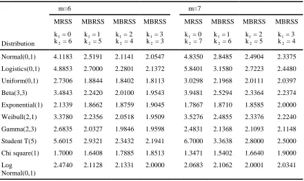
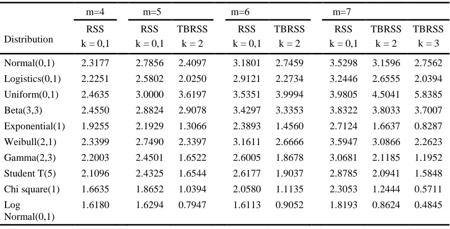
The REs of mean estimators are reported in Tables1-3. Calculation were done using Eqs (17) and (18) for different values of k₁ and k for MBRSS and TBRSS respectively with

m = 4,5,6,7. The results advocate the efficiency of MBRSS over SRS for estimating

superior to MBRSS in most of the considered symmetric distributions, except logistc(0,1). But this loss in efficiency decreases as m increases with minimum loss occurs when k = 1.₁ Therefore, it can be concluded that in the situation of scarcity of resources the experimenter should prefer MBRSS.

Table 1: RE of MBRSS vs SRS for estimating population mean for m = 4,5

m=4 m=5

MRSS MBRSS MBRSS MRSS MBRSS MBRSS

Distribution

1 2

k = 0

k = 4 12

k = 1

k = 3 12

k = 2

k = 2 12

k = 0

k = 5 12

k = 1

k = 4 12

k = 2 k = 3

Normal(0,1) 2.8000 1.7160 1.5000 3.5063 2.0557 1.8242

Logistics(0,1) 3.1680 1.8136 1.4343 4.1903 2.2191 1.9657

Uniform(0,1) 2.0894 1.4245 1.5025 2.2876 1.7087 1.6128

Beta(3,3) 2.5000 1.6144 1.5094 3.0000 1.8960 1.7254

Exponential(1) 2.3751 1.7000 1.3496 2.2354 1.9165 1.7777

Weibull(2,1) 2.5348 1.6549 1.4860 3.0000 1.9577 1.8010

Gamma(2,3) 2.5593 1.7037 1.4000 2.6143 1.9259 1.8000

Student T(5) 3.6000 2.0000 1.4198 4.6853 2.3575 2.0000

Chi square(1) 2.3753 1.7276 1.2357 1.9000 1.8795 1.7584

Log Normal(0,1) 3.2091 2.2177 1.2309 2.7809 2.3147 1.8651

Table 2: RE of MBRSS vs SRS for estimating population mean for m = 6, 7

m=6 m=7

MRSS MBRSS MBRSS MBRSS MRSS MBRSS MBRSS MBRSS

Distribution

1 2

k = 0

k = 6 12

k = 1

k = 5 12

k = 2

k = 4 12

k = 3

k = 3 12

k = 0

k = 7 12

k = 1

k = 6 12

k = 2

k = 5 12

k = 3 k = 4

Normal(0,1) 4.1183 2.5191 2.1141 2.0547 4.8350 2.8485 2.4904 2.3375

Logistics(0,1) 4.8853 2.7000 2.2801 2.1372 5.8401 3.1580 2.7223 2.4480

Uniform(0,1) 2.7306 1.8844 1.8402 1.8113 3.0298 2.1968 2.0111 2.0397

Beta(3,3) 3.4843 2.2420 2.0100 1.9543 3.9481 2.5294 2.3364 2.2374

Exponential(1) 2.1339 1.8662 1.8759 1.9045 1.7867 1.8710 1.8585 2.0000

Weibull(2,1) 3.3780 2.2356 2.0518 1.9509 3.5276 2.4855 2.3376 2.2240

Gamma(2,3) 2.6835 2.0327 1.9846 1.9598 2.4831 2.1368 2.1093 2.1148

Student T(5) 5.6015 2.9321 2.3432 2.1941 6.7000 3.3638 2.8000 2.5000

Chi square(1) 1.7000 1.6408 1.7885 1.8513 1.3471 1.5402 1.6640 1.9000

Log Normal(0,1)

Table 3: RE of TBRSS vs SRS for estimating population mean for m = 4,5, 6, 7

Distribution

m=4 m=5 m=6 m=7

RSS

k = 0,1

RSS

k = 0,1

TBRSS

k = 2

RSS

k = 0,1

TBRSS

k = 2

RSS

k = 0,1

TBRSS

k = 2

TBRSS k = 3

Normal(0,1) 2.3177 2.7856 2.4097 3.1801 2.7459 3.5298 3.1596 2.7562

Logistics(0,1) 2.2251 2.5802 2.0250 2.9121 2.2734 3.2446 2.6555 2.0394

Uniform(0,1) 2.4635 3.0000 3.6197 3.5351 3.9994 3.9805 4.5041 5.8385

Beta(3,3) 2.4550 2.8824 2.9078 3.4297 3.3353 3.8322 3.8033 3.7007

Exponential(1) 1.9255 2.1929 1.3066 2.3893 1.4560 2.7124 1.6637 0.8287

Weibull(2,1) 2.3399 2.7490 2.3397 3.1611 2.6666 3.5947 3.0866 2.2623

Gamma(2,3) 2.2003 2.4501 1.6522 2.6005 1.8678 3.0681 2.1185 1.1952

Student T(5) 2.1096 2.4325 1.6544 2.6177 1.9037 2.8785 2.0941 1.5848

Chi square(1) 1.6635 1.8652 1.0394 2.0580 1.1135 2.3053 1.2444 0.5711

Log Normal(0,1)

1.6180 1.6294 0.7947 1.6113 0.9052 1.8193 0.8624 0.4845

4. Estimation of population median

Median is reliable measure of center tendency when underlying distribution is asymmetric or highly skewed. We define median estimators based on SRS, TBRSS and MBRSS. An extensive simulation study is also conducted to compare the efficiency of the median estimators based on TBRSS and MBRSS relative to conventional estimator based on SRS. Let X , X , X ,. . ., X1 2 3 m be a SRS of size m. Then SRS estimator of population median, say, is defined as

((m+1)/ 2:m)

((m/ 2):m) (((m+2)/ 2):m) SRS

X if m is odd

X + X

θ =

if m is even 2

ˆ _



The population median estimator under TBRSS is defined by

i(1:k) i(i:m-k) TBRSS

i((m:m)

X

i = 1, 2,. . ., k

X i = k +1, k + 2,. . ., m - 2k

θ = Median

X i = m - 2k +1,. . ., m

ˆ

    

Similarly, Suppose that k2 is even and

k2 k2 k2 k2

1 1 1 1 1 _{2 2 2}

2 2 2 2

1(1:k ) 2(2:k ) k (k :k ) _{1( :k ) 2( :k ) ( :k )}

X , X ,. . ., X , X , X ,. . ., X ,

2 2 2 2 2 2

(k +2)/2((k +2)/2:k ) k ((k +2)/2:k )

X ,. . ., X be

MBRSSe of size m. Then the population median estimator is given by

1

1 2 2 2

2 2

2 2 2

i(i:k )

k i(k / 2:k ) ₂ MBRSSe

k k

i((k +2)/ 2:k ) 2 2

X _{i = 1, 2,. . ., k}

X i = 1, 2,. . .,

θ = Median

X i = ( ) +1 + ( ) + 2,. . ., k

ˆ

Suppose that k₂ is odd and X1(1:k )₁ , X2(2:k )₁ ,. . ., Xk (k :k )_{1 1 1} , X2((k +1)/2:k )_{2 2} ,. . ., Xk ((k +1)/2:k )_{2 2 2} be MBRSSo of size m. Then the population median estimator is given by

1 1

2 2 2

i(i:k ) MBRSSo i((k +1)/ 2:k )

i = 1, 2,. . ., k X

θ = Median X i = 1,2,. . .,k

ˆ 



The REs of θˆMBRSS and θˆTBRSSwith respect to θˆSRS are defined as

 

SRS MBRSS SRS

MBRSS SRS TBRSS SRS

TBRSS

MSE(θ )

eff(θ ,θ ) = 19

MSE(θ )

MSE(θ )

eff(θ ,θ ) =

MSE(θ )

ˆ

ˆ ˆ

ˆ

ˆ

ˆ ˆ

ˆ 20 

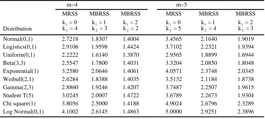
REs of the median based on MBRSS and TBRSS with respect to the median estimator based on SRS are presented in Tables4 6 under both symmetric and asymmetric distributions. REs are calculated using Eq(19) and Eq(20). The simulated median and its

MSE based on 4

4×10 simulation are defined as:

40000 40000

2

S S,i S S,i

i=1 i=1

1 1

θ = θ MSE(θ ) = (θ - θ) S = SRS,TBRSS,MBRSS

40000 40000

ˆ _ ˆ ˆ _ ˆ

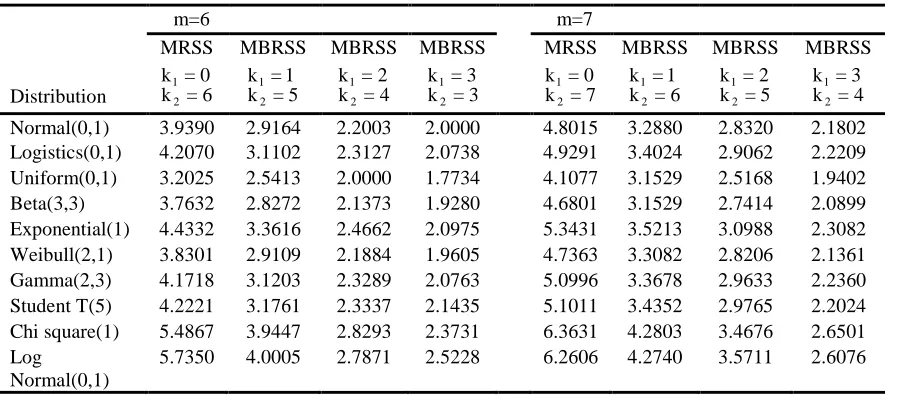
We can see from Tables4 5 that a substantial gain in efficiency is obtained by using MBRSS relative to SRS for estimating median for symmetric and asymmetric distributions. RE increases with increase in m. However, maximum gain in efficiency is obtained at k = 01 . The Table6 reflects efficiency of TBRSS for estimating population median. It can be seen from Tables4-6 that the proposed MBRSS is superior to TBRSS for estimating population median for both symmetric and asymmetric distributions. For instance, RE of median estimator under MBRSS for m=5 at k = 1₁ is 2.1640, while it is 1.5330 under TBRSS for the case of normal distribution (0,1). Therefore, the results suggest that MBRSS is economical and efficient alternative to TBRSS for estimating population median.

Table 4: RE of MBRSS vs SRS for estimating population median for m= 4,5

m=4 m=5

MRSS MBRSS MBRSS MRSS MBRSS MBRSS

Distribution 12

k = 0

k = 4 1₂

k = 1

k = 3 1₂

k = 2

k = 2 1₂

k = 0

k = 5 1₂

k = 1

k = 4 1₂

k = 2 k = 3

Normal(0,1) 2.7218 1.8307 1.4004 3.4565 2.1640 1.9019

Logistics(0,1) 2.9106 1.9598 1.4424 3.7102 2.2321 1.9394

Uniform(0,1) 2.2222 1.6140 1.3870 2.9565 1.8899 1.6944

Beta(3,3) 2.5547 1.7800 1.4031 3.3204 2.0850 1.8048

Exponential(1) 3.2580 2.0646 1.4061 4.0571 2.3748 2.0345

Weibull(2,1) 2.6284 1.8388 1.4035 3.5132 2.1184 1.8738

Gamma(2,3) 2.8860 1.9246 1.4207 3.7487 2.2507 1.9615

Student T(5) 3.0245 2.0007 1.4722 3.6789 2.2673 1.9304

Chi square(1) 3.8056 2.5000 1.4188 4.9024 2.6796 2.3289

Table 5: RE of MBRSS vs SRS for estimating population median for m = 6, 7

m=6 m=7

MRSS MBRSS MBRSS MBRSS MRSS MBRSS MBRSS MBRSS

Distribution 12

k = 0

k = 6 1₂

k = 1

k = 5 1₂

k = 2

k = 4 1₂

k = 3

k = 3 1₂

k = 0

k = 7 1₂

k = 1

k = 6 1₂

k = 2

k = 5 1₂

k = 3 k = 4

Normal(0,1) 3.9390 2.9164 2.2003 2.0000 4.8015 3.2880 2.8320 2.1802

Logistics(0,1) 4.2070 3.1102 2.3127 2.0738 4.9291 3.4024 2.9062 2.2209

Uniform(0,1) 3.2025 2.5413 2.0000 1.7734 4.1077 3.1529 2.5168 1.9402

Beta(3,3) 3.7632 2.8272 2.1373 1.9280 4.6801 3.1529 2.7414 2.0899

Exponential(1) 4.4332 3.3616 2.4662 2.0975 5.3431 3.5213 3.0988 2.3082

Weibull(2,1) 3.8301 2.9109 2.1884 1.9605 4.7363 3.3082 2.8206 2.1361

Gamma(2,3) 4.1718 3.1203 2.3289 2.0763 5.0996 3.3678 2.9633 2.2360

Student T(5) 4.2221 3.1761 2.3337 2.1435 5.1011 3.4352 2.9765 2.2024

Chi square(1) 5.4867 3.9447 2.8293 2.3731 6.3631 4.2803 3.4676 2.6501

Log Normal(0,1)

5.7350 4.0005 2.7871 2.5228 6.2606 4.2740 3.5711 2.6076

Table 6: RE of TBRSS vs SRS for estimating population median for m = 4,5, 6, 7

Distribution

m=4 m=5 m=6 m=7

RSS

k = 0,1

RSS

k = 0,1

TBRSS

k = 2

RSS

k = 0,1

TBRSS

k = 2

RSS

k = 0,1

TBRSS

k = 2

TBRSS k = 3

Normal(0,1) 2.1963 2.0775 1.5330 2.7458 2.2223 2.5118 2.1181 1.3169

Logistics(0,1) 2.2450 2.1804 1.5555 2.8337 2.3288 2.5905 2.2001 1.3184

Uniform(0,1) 1.9933 1.8778 1.4129 2.4304 2.1036 2.2164 1.9441 1.2532

Beta(3,3) 2.1335 2.0048 1.6021 2.6048 2.3500 2.4562 2.0521 1.5021

Exponential(1) 2.3033 2.3185 1.6350 2.9416 2.2449 2.6840 2.3080 1.3609

Weibull(2,1) 2.1986 2.0819 1.5059 2.5761 2.2387 2.4261 2.1567 1.3116

Gamma(2,3) 2.2174 2.1531 1.7526 2.4321 2.1427 2.5868 2.2331 1.3021

Student T(5) 2.3249 2.1971 1.5695 2.8289 2.2796 2.5331 2.2219 1.3300

Chi square(1) 2.4542 2.6091 1.7705 2.1814 2.3845 3.1269 2.6386 1.4534

Log Normal(0,1)

2.6950 2.6776 1.7754 3.2401 2.4455 3.1572 2.6809 1.4262

5. Weighted MBRSS for skewed distribution

To improve the efficiency of MBRSS scheme in estimating population mean when underlying distribution is asymmetric, a weighted MBRSS for even k₂ is defined as

k 2

1 2 2

k

i1 1 11 2 ₂ 21 2 2

2 ₂

k k

wMBRSSe i(i:k ) _{i( :k )} i((k +2)/ 2):k ) i=1 i=1 i=(k +2)/ 2

X = ( w X +w X +  w X ) (21)

Similarly, a weighted MBRSS for odd k2 is defined as

1 2

i2 1 12 2 2

k k

wMBRSSo i(i:k ) i(((k +1)/ 2):k )

i=1 i=1

X = ( w X + w X ) (22)

estimator. The optimal weights, which provide a measure of uncertainty, can be found by using entropy measure from information theory. Entropy is considered as a measure of uncertainty. A simple choice of this measure is Shannon's entropy:

m

i1 i1 i=1

H(w) = - w ln(w ) (23)

where m

i=1w ln(w ) = 0i1 i1 w = 0i1

 and H(w) reaches at maximum when

11 21 31 m1

1

w = w = w = = w =

m

L . Then maximizing Eq(23) subject to the constraints

m i=1w = 1i1

 leads to optimal solution. This problem can be expressed as a nonlinear system m

i1 i1 i=1

Maximize - w ln(w )

subject to the constraints

1. 1 2 k

i1 11 2 21 ₂ 2

k

i ((k +2)/ 2)

i=1 _{( )}

k

w μ + (w μ + w μ ) = μ

2  



2. m i=1w = 1i1

 where 2 j1 11 2 2 j1 21 k 2 k k 2 2 2

w = w j = 1, 2,3,. . .,

w = w j = ( ) +1, ( ) + 2,. . ., k

  

  

To find weights, the Lagrange function is formulated as 1

2

i1 i1 i1 11 ₂ 21 ₂ i1

k

m m

*

1 i (k / 2) ((k +2)/ 2) 2

i=1 i=1 i=1

k

L = - w ln(w ) + λ (μ - w μ - (w μ + w μ )) + λ (1- w )

2  

  

Solving the first order conditions, the solution leads to

1 ₂

11 ₁

1 1

2 2 2 1 i

1 ₂ 21

1

1 1

2 2 2 1 i

1 j

1

1 1

2 2 2 1 i

-λ μ(k /2)

k -λ μ -λ μ

k (k / 2) ((k +2)/ 2) -λ μ 2

i=1 -λ μ ((k +2)/2)

k -λ μ -λ μ

k (k / 2) ((k +2)/ 2) -λ μ 2

i=1 -λ μ

i1 _k 1

-λ μ -λ μ

k (k / 2) ((k +2)/ 2) -λ μ 2

i=1

e w =

(e + e ) + e

e w =

(e + e ) + e

e

w = , j = 1, 2,. . ., k

(e + e ) + e

ˆ ˆ ˆ     

where λ1 is Lagrangian multiplier. Then the unbiased estimator will be recovered through the estimated weights by

1 2 2

i1 ₁ 11 ₂ 21 _{2 2}

2

k k / 2 k

wMBRSSe i(i:k ) i((k / 2):k )₂ i((k +2)/ 2):k )

i=1 i=1 i=(k +2)/ 2

X = ( w Xˆ + w Xˆ +  w Xˆ )

and its associated weighted variance is given by

1

2

i1 1 11 2 2 21 2 2 k

2 2 2

wMBRSSe ₂ (i:k ) ₂ (k / 2:k ) (k +2)/ 2:k ) i=1

1 k

Var(X ) = w σ + (w σ + w σ )

We, now, find weights for the estimator X_wMBRSSo defined above. where w12 and

i2 1

w ,i = 1, 2,. . ., k are non negative weights to be chosen such that X_wMBRSSo is unbiased estimator. In this case, the problem can be expressed as a nonlinear system

m

i2 i2 i=1

Maximize - w ln(w )

subject to the constraints

1. 1

i2 2 12 2 k

i ((k +1)/2)

i=1w μ + k w μ = μ



2. i2 m

i=1w = 1



where w = w j = 1, 2,. . ., kj2  12 2

To find weights, the Lagrange function is formulated as

1

i2 i2 1 i2 2 12 ₂ 2 i2

k

m m

*

i ((k +1)/ 2)

i=1 i=1 i=1

L = - w ln(w ) + λ (μ - w μ - k w μ& ) + λ (1- w )

Solving the first order conditions, the solution leads to

1 ₂ 12

1 1 2+1 1 i

1 1 1 2+1 1 i

-λ μ(k +1/2) k -λ μ_{(k / 2) -λ μ} k 2

i=1 -λ μi

i2 _{-λ μ} k 1

-λ μ (k / 2)

k 2

i=1

e w =

e + e

e

w = , i = 1, 2,. . ., k

e + e

ˆ

ˆ







where λ1 is Lagrangian multiplier. Then the unbiased estimator will be recovered through the estimated weights by

1 2

i2 12 2 2

k k

wMBRSSo i(i:k )₁ i(((k +1)/ 2):k )

i=1 i=1

X = ( w Xˆ +w Xˆ )

and its associated weighted variance is given by

1

2 12

1 2 2

k

2 2

wMBRSSo ₂ i2 (i:k ) ₂ (((k +1)/ 2):k ) i=1

1 k

Var(X ) = w σ + w σ

m ˆ m ˆ

5.1 Weighted TBRSS for skewed distribution

The population mean estimator based on weighted TBRSS (wTBRSS)is defined by

  m-k

wTBRSS 1 (1:m) j (j:m) m m:m i=k+1

X = (kw Xˆ +  w Xˆ + kw Xˆ ) (24)

and its associated weighted variance is given by

m-k

2 2 2

wTBRSS 1 (1:m) m (m:m) j (j:m)

i=k+1

k 1

Var(X ) = (w σ + w σ ) + w σ

The weights w (j = 1, 2,3,. . ., m)j are estimated using Shannon's entropy, for details see Al-Nasser and Al-Omari (2015), and given by

 

   

 

1 1:m

1 (1:m) 1 (m:m) 1 i:m 1 m:m

1 (1:m) 1 (m:m) 1 i:m -λ μ

1 _m-κ

-λ κμ -λ κμ -λ μ i=κ+1 -λ μ

m _{-λ κμ -λ κμ} m-κ _{-λ μ} i=κ+1

e w =

κ(e + e ) + e

e

w =

κ(e + e ) + e

ˆ

ˆ





and

 

 

j m:m

1 (1:m) 1 (m:m) 1 i:m -λ μ

j _{-λ kμ -λ kμ} m-k _{-λ μ} i=k+1

e

w = , j = k +1, k + 2,. . ., m - k

k(e + e ) +  e

The REs of wMBRSS and wTBRSS with respect to SRS for estimating mean are given by

SRS wMBRSS SRS

wMBRSS

Var(X )

RE(X , X ) =

Var(X ) (25)

and

SRS wTBRSS SRS

wTBRSS

Var(X )

RE(X , X ) =

Var(X ) (26)

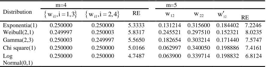
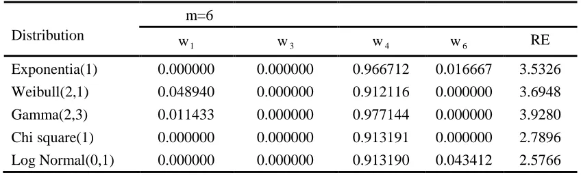
The numerical values of REs of wMBRSS and wTBRSS with respect to SRS are reported in Tables7-10 for different asymmetric distributions, assuming k = 21 and k = 2, for wMBRSS and wTBRSS respectively and sample size m = 4,5,6. The results indicate significant improvement in the efficiency of mean estimator by using wMBRSS. Moreover, RE increases as mgets large. For instance, REs of unweighted MBRSS for

m = 4,5 at k = 21 are 1.3496 and 1.7777 respectively, as given in Table1 for the case of exponential(1) distribution. While, these are 5.3333 and 7.2246 under wMBRSS as given in Table7. A gain in efficiency is also obtained by using wTBRSS. For example, REs of unweighted TBRSS for m = 5 at k = 2 are 1.3066 and for the case of exponential(1) distribution. While, it is 2.7111 under wTBRSS as indicated in Tables9 . However, a substantial gain in efficiency of mean estimator is obtained by using wMBRSS instead of wTBRSS as indicated for the case of exponential (1) distribution.

Table 7: Optimal weights and RE of wMBRSS vs SRS for estimating mean of asymmetric population for m = 4,5

Distribution

m=4 m=5









Exponentia(1) 0.250000 0.250000 5.3333 0.131214 0.315600 0.184402 7.2246

Weibull(2,1) 0.249997 0.250003 5.8317 0.245521 0.297510 0.152321 8.0235

Gamma(2,3) 0.250003 0.249997 5.5650 0.182654 0.303214 0.171440 7.5747

Chi square(1) 0.250000 0.250000 5.0166 0.062997 0.340050 0.198886 7.4161

Log Normal(0,1)

Table 8: Optimal weights and RE of wMBRSS vs SRS for estimating mean of asymmetric population for m = 6

Distribution

m=6

11

w w21 w11 w21 RE

Exponentia(1) 0.500000 0.500000 0.000000 0.000000 8.0000

Weibull(2,1) 0.500006 0.499994 0.000000 0.000000 8.7465

Gamma(2,3) 0.500000 0.500000 0.000000 0.000000 8.3468 Chi square(1) 0.500000 0.481383 0.259308 0.000000 8.0434

Log

Normal(0,1)

0.500000 0.430505 0.000000 0.284747 8.8792

Table 9: Optimal weights and RE of wTBRSS vs SRS for estimating mean of asymmetric population for m = 4,5

Distribution

m=4 m=5

1

w w4 RE w1 w3 w5 RE

Exponentia(1) 0.295451 0.204542 1.6147 0.107040 0.558210 0.113854 2.7111

Weibull(2,1) 0.265641 0.234345 2.1205 0.093912 0.611774 0.100233 2.8000

Gamma(2,3) 0.282100 0.217927 1.7790 0.101222 0.579425 0.109165 2.4456

Chi square(1) 0.312914 0.187140 1.4266 0.114632 0.536312 0.117324 1.8378

Log Normal(0,1)

0.377238 0.122800 1.5536 0.137000 0.514632 0.105653 1.7567

Table 10: Optimal weights and RE of wTBRSS vs SRS for estimating mean of asymmetric population for m = 6

Distribution

m=6

1

w w 3 w 4 w 6 RE

Exponentia(1) 0.000000 0.000000 0.966712 0.016667 3.5326

Weibull(2,1) 0.048940 0.000000 0.912116 0.000000 3.6948

Gamma(2,3) 0.011433 0.000000 0.977144 0.000000 3.9280

Chi square(1) 0.000000 0.000000 0.913191 0.000000 2.7896

Log Normal(0,1) 0.000000 0.000000 0.913190 0.043412 2.5766

6. Simulation study

In this section, effectiveness of the proposed MBRSS scheme relative to the traditional SRS scheme is ascertained in the presence of outlier for mequal to 4,5,6 and 7 with

1

k = 1, 2.The idea is to replace minimum value of the first sample in one of the two data

quartile and IQR is the interquartile range. For k = 11 , minimum value in the first sample of second data set k2 is replaced with X(1). For k1= 2, the minimum value in first

sample of the first data set k1 is replaced with X(1).The simulation study is carried out for different symmetric and asymmetric distributions such as normal(0,1), logistic(0,1), uniform(0,1), beta(3,3), exponential(1), weibull(2,1), gamma(2,3) and student t(5). The performance of the estimators is investigated by comparing simulated mean square error(MSE) as a criteria of robustness of the mean and median estimators. The MSE based on 40,000 simulation is defined as:

40,000

2

h h,i

i=1

1

MSE(μ ) = (μ - μ) h = SRS,MBRSS

40,000

ˆ  ˆ

The estimated REs of MBRSS vs SRS based on MSEs for estimating mean and median of considered distributions are depicted in Figures1- 2. The Figure1 indicates that the RE of MBRSS vs SRS, for estimating mean, is increasing with increase in mexcept some skewed distributions such as exponential(1) and gamma(2,3) wherein RE decreases as m increases when one unit (k = 11 ) is chosen by SRS and remaining by MRSS. For the choice k = 21 i.e. two units are selected by RSS and remaining by MRSS, RE increases when mgets large under all considered distributions. However, it is observed that maximum gain in efficiency is obtained when one unit of a sample is taken by SRS i.e.

1

k = 1 and remaining (k = m - k )2 1 units by MRSS scheme.The Figure.2 also indicates that MBRSS is superior to the traditional SRS for estimating median of a population even in the presence of outliers. The choice k = 11 also remains optimum in case of median estimation.

Figure 2: REs of median estimators based on MBRSS vs SRS in presence of outliers for symmetric and asymmetric distributions

7. Ranking with concomitant variable

In many practical problems the variable of interest, X, is hard to measure and difficult to rank as well but a concomitant variable, Y, correlated with, X, can easily be measured. Then the concomitant variable can be used for the ranking of the sampling units. For instance, the assessment of the status of hazard waste sites is usually costly. But, often, a great deal of knowledge about hazard waste sites can be obtained from records, photos etc. and then be used to rank the hazard waste sites. In this section, we follow Stokes (1977) idea in which ranking is performed using concomitant variable,say Y, that can be

measured easily. Stokes (1977) proposed the following model with the assumptions (1)

the regression of X on Y is linear (2) the underlying distributions of standardized

variables Y Y

  

Y

and X X

 



X

are same.

X

i[i:m]j X i(i:m)j Y ij

Y

σ

X = μ + ρ (Y - μ ) + ε ,i = 1,2,. . .,m; j = 1,2,. . .,r

σ (27)

Here, Yi(i:m) and





2 2 2

ε X

σ = σ (1- ρ ). And Xi[i:m]j is the ith smallest value of X corresponding to ithsmallest value of Y i.e.

i(i:m)

Y in jth replication

7.1 Estimation under imperfect ranking

MBRSSe estimator of population mean using concomitant variableY i.e. X_MBRSSCe is defined as

1 2 2

2 2 2 2

2

k k / 2 k

r r r

MBRSSCe i[i:k ]j₁ i[k / 2:k ]j i[(k +2)/ 2:k ]j j=1i=1 j=1 i=1 j=1i=(k / 2)+1

1

X = ( X + X + X )

mr      (28)

It is easy to show that X_MBRSSCe is unbiased estimator of μ_X and its variance is given by 1

1 2 2

2 _k X

2 2 2 2 2

MBRSSCe ₂ X ₂ Y(i:k ) 2 Y(k / 2:k )

i=1 Y

1 σ

Var(X ) = mσ (1- ρ ) + ρ ( σ + k σ )

m r σ

 



 

  (29)

Similarly, the estimator XMBRSSCo is defined as

1 2

1 2 2

k k

r r

MBRSSCo i[i:k ]j i[(k +1)/ 2:k ]j j=1i=1 j=1i=1

1

X = ( X + X )

mr   (30)

It is also easy to show that X_MBRSSCo is unbiased estimator of μ_X and its variance is given by

1

2

1 2 2

2 _k X

2 2 2 2 2

MBRSSCo ₂ X ₂ Y(i:k ) Y((k +1)/ 2:k )

i=1 Y

1 σ

Var(X ) = mσ (1- ρ ) + ρ ( σ + k σ )

m r σ

 



 

  (31)

The estimator X_TBRSSC is defined as

r k r m-k r m

TBRSSC i[1:m]j i[i:m]j i[m:m]j j=1i=1 j=1i=k+1 j=1i=(m-k+1

1

X = ( X + X + X )

mr      (32)

and its variance is given by

2 _m-k

X

2 2 2 2 2

TBRSSC ₂ X ₂ Y(1:m) Y(i:m)

i=k+1 Y

1 σ

Var(X ) = mσ (1- ρ ) + ρ (2kσ + σ )

m r σ

 



 

  ₍₃₃₎

Lemma-2: The estimator XMBRSSC is more efficient than XSRS i.e.

MBRSSC SRS

Var(X )Var(X )

Proof: From Eq(29), we have

1

2

1 2 2

1

2

1 2 2

2 _k X

2 2 2 2 2

MBRSSCe ₂ X ₂ Y(i:k ) Y(k / 2:k )

i=1 Y

2 _k

X

2 2 2 2 2 2

X 1 Y Y(i:k ) Y Y(k / 2:k )

2 2

i=1 Y

1 σ

Var(X ) = mσ (1- ρ ) + ρ ( σ + k σ )

m r σ

1 σ

= mσ (1- ρ ) + ρ (k σ - (μ - μ ) + k σ )

m r σ

              1

1 1 2

1 1 1

2 _k

X

2 2 2 2 2 2 2 2

X Y Y(i:k ) Y Y T(j:m) T

2 2

i=1 Y

2 _k

X

2 2 2 2 2

X Y Y(i:k ) Y

2 2

i=1 Y

2 2 _k

X 2 X

MBRSSCe _{2 2}

i=1 Y

1 σ

mσ (1- ρ ) + ρ (k σ - (μ - μ ) + k σ ) σ σ

m r σ

1 σ

mσ (1- ρ ) + ρ (mσ - (μ - μ ) )

m r σ

σ σ

Var(X ) - ρ (μ

mr m rσ

                   Q 1 2 Y(i:k )- μ ) Y

Note that the second term on right hand side is non negative. Hence,

MBRSSCe SRS

Now, from Eq(31), we have

1

1 2 2

1

1 ₁ 2 _{2 2}

2 _k X

2 2 2 2 2

MBRSSCo 2 X 2 Y(i:k ) 2 Y((k +1)/ 2:k )

i=1 Y

2 _k

X

2 2 2 2 2 2

X Y Y(i:k ) Y Y((k +1)/ 2:k )

2 2

i=1 Y

1 σ

Var(X ) = mσ (1- ρ ) + ρ ( σ + k σ )

m r σ

1 σ

= mσ (1- ρ ) + ρ (k σ - (μ - μ ) + k σ )

m r σ

 



 

 

 



 

 

1

1 ₁

1 1

2 k

X

2 2 2 2 2 2 2 2

X Y Y(i:k ) Y 2 Y T(j:m) T

2 2

i=1 Y

2 k

X

2 2 2 2 2

X Y Y(i:k ) Y

2 2

i=1 Y

2 2 _k

X 2 X

MBRSSCo _{2 2}

i=1 Y

1 σ

mσ (1- ρ ) + ρ (k σ - (μ - μ ) + k σ ) σ σ

m r σ

1 σ

mσ (1- ρ ) + ρ (mσ - (μ - μ ) )

m r σ

σ σ

Var(X ) - ρ

mr m rσ

 

    

 

 

   

 



Q

1 1

2 Y(i:k ) Y

(μ - μ )



Here, we also note that the second term on right hand side is non negative. This completes the proof. The REs of XMBRSSC and XTBRSSC _{with respect to} XSRS are given by

SRS J SRS

J

Var(X )

RE(X , X ) = ;J = MBRSSC,TBRSSC

Var(X ) (34)

The performance of MBRSSC and TBRSSC for estimating population mean and median are investigated when the study variable X and auxiliary variable Y follow standard bivariate normal distribution with pdf as given by

2 2

2 2

1 (x - 2ρxy + y )

f(x, y) = exp - , - < x, y <

2(1- ρ ) 2π 1- ρ

 

 

 

 

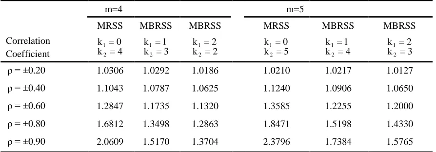
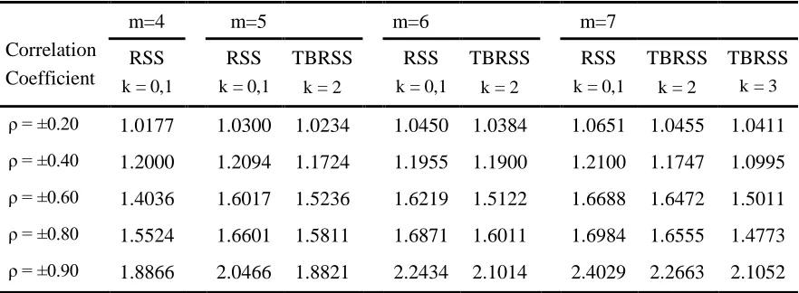
The simulated REs of mean and median estimators for m = 4,5,6,7 with different values of correlation coefficient ρ = ±0.20,±0.40,±0.60,±0.80,±0.90 are calculated using Eq(34)

after 4

4×10 replication and reported in Tables 11-16. As expected, the performance of the mean and median estimators depend on value of correlation coefficient. The estimators become more precise as correlation increases and vice-versa. The MBRSSC is less efficient than TBRSSC for estimating population mean. But this loss is not so large as we can see from Table11-16. For example, if m = 5 the RE of MBRSSC for estimating mean is 1.2255 for k = 1₁ ,ρ = ±0.60. While, it is 1.5236 under TBRSSC for k = 2. However, MBRSSC performs better than TBRSSC in estimating population median for

1

Table 11: RE of MBRSSC vs SRS for estimating mean for standard bivariate normal distribution for m = 4,5

m=4 m=5

MRSS MBRSS MBRSS MRSS MBRSS MBRSS

Correlation Coefficient

1 2

k = 0

k = 4 12

k = 1

k = 3 12

k = 2

k = 2 12

k = 0

k = 5 12

k = 1

k = 4 12

k = 2 k = 3

ρ = ±0.20 1.0306 1.0292 1.0186 1.0210 1.0217 1.0127

ρ = ±0.40 1.1043 1.0787 1.0625 1.1240 1.0906 1.0650

ρ = ±0.60 1.2847 1.1735 1.1320 1.3585 1.2255 1.2000

ρ = ±0.80 1.6812 1.3498 1.2863 1.8471 1.5198 1.4330

ρ = ±0.90 2.0609 1.5170 1.3704 2.3796 1.7384 1.5765

Table 12: RE of MBRSSC vs SRS for estimating mean for standard bivariate normal distribution for m = 6, 7

m=6 m=7

MRSS MBRSS MBRSS MBRSS MRSS MBRSS MBRSS MBRSS

Correlation Coefficient

1 2

k = 0

k = 6 1₂

k = 1

k = 5 1₂

k = 2

k = 4 1₂

k = 3

k = 3 1₂

k = 0

k = 7 1₂

k = 1

k = 6 1₂

k = 2

k = 5 1₂

k = 3 k = 4

ρ = ±0.20 1.0186 1.0272 1.0235 1.0054 1.0267 1.0261 1.0213 1.0494

ρ = ±0.40 1.3353 1.1093 1.1083 1.0728 1.1641 1.1021 1.1096 1.1170

ρ = ±0.60 1.3702 1.2837 1.2462 1.2391 1.3861 1.3222 1.2780 1.2633

ρ = ±0.80 1.9310 1.6145 1.5071 1.5153 2.0280 1.7028 1.6233 1.5641

ρ = ±0.90 2.6000 1.9341 1.7790 1.7097 2.8000 2.1170 1.9571 1.8583

Table 13: RE of MBRSSC vs SRS for estimating median for standard bivariate normal distribution for m = 4,5

m=4 m=5

MRSS MBRSS MBRSS MRSS MBRSS MBRSS

Correlation Coefficient

1 2

k = 0

k = 4 12

k = 1

k = 3 12

k = 2

k = 2 12

k = 0

k = 5 12

k = 1

k = 4 12

k = 2 k = 3

ρ = ±0.20 1.0271 1.0168 1.0242 1.0230 1.0240 1.0096

ρ = ±0.40 1.1011 1.0683 1.0525 1.1345 1.0751 1.0898

ρ = ±0.60 1.3000 1.1806 1.1046 1.3498 1.1915 1.1617

ρ = ±0.80 1.6305 1.3902 1.2263 1.8727 1.3869 1.3849

ρ = ±0.90 2.0027 1.5870 1.3000 2.3769 1.5861 1.5850

m=6 m=7

MRSS MBRSS MBRSS MBRSS MRSS MBRSS MBRSS MBRSS

Correlation Coefficient

1 2

k = 0

k = 6 12

k = 1

k = 5 12

k = 2

k = 4 12

k = 3

k = 3 12

k = 0

k = 7 12

k = 1

k = 6 12

k = 2

k = 5 12

k = 3 k = 4

ρ = ±0.20 1.0188 1.0006 1.0270 1.0180 1.0244 1.0228 1.0401 1.0221

ρ = ±0.40 1.1438 1.1076 1.0911 1.0989 1.1309 1.1079 1.0969 1.0658

ρ = ±0.60 1.3824 1.2598 1.2040 1.2001 1.3948 1.3205 1.2529 1.2183

ρ = ±0.80 1.9478 1.6564 1.5000 1.4258 2.0355 1.7321 1.6287 1.4844

ρ = ±0.90 2.5325 2.1023 1.7474 1.6594 2.8433 2.2178 2.0468 1.7106

Table 15: RE of TBRSSC vs SRS for estimating mean for standard bivariate normal distribution

Correlation Coefficient

m=4 m=5 m=6 m=7

RSS k = 0,1

RSS k = 0,1

TBRSS k = 2

RSS k = 0,1

TBRSS k = 2

RSS k = 0,1

TBRSS k = 2

TBRSS k = 3

ρ = ±0.20 1.0177 1.0300 1.0234 1.0450 1.0384 1.0651 1.0455 1.0411

ρ = ±0.40 1.2000 1.2094 1.1724 1.1955 1.1900 1.2100 1.1747 1.0995

ρ = ±0.60 1.4036 1.6017 1.5236 1.6219 1.5122 1.6688 1.6472 1.5011

ρ = ±0.80 1.5524 1.6601 1.5811 1.6871 1.6011 1.6984 1.6555 1.4773

ρ = ±0.90 1.8866 2.0466 1.8821 2.2434 2.1014 2.4029 2.2663 2.1052

Table 16: RE of TBRSSC vs SRS for estimating median for standard bivariate normal distribution.

Correlation Coefficient

m=4 m=5 m=6 m=7

RSS

k = 0,1

RSS

k = 0,1

TBRSS

k = 2

RSS

k = 0,1

TBRSS

k = 2

RSS

k = 0,1

TBRSS

k = 2

TBRSS k = 3

ρ = ±0.20 1.0090 1.0160 1.0127 1.0310 1.0215 1.0338 1.0250 1.0140

ρ = ±0.40 1.1002 1.1048 1.0788 1.1151 1.0956 1.1500 1.0806 1.0165

ρ = ±0.60 1.3024 1.3225 1.2500 1.4391 1.4030 1.4437 1.1229 1.0151

ρ = ±0.80 1.5229 1.6099 1.5339 1.9856 1.6079 1.8751 1.2422 1.0241

8. Illustration with real data

In this section we use a real data set to illustrate the efficiency of the proposed MBRSS and TBRSS schemes with respect to SRS in estimating mean and median height of 399 conifer trees.The data based on two variables: X, the diameter in centimeters at breast

height, and Y, the entire height in feet, for more detail see Platt et al. (1988). The

summary statistics of the two variables are given by

399 2 399 2

i=1 i=1

X i X i X X X

399 2 399 2

i=1 i=1

Y i Y i Y Y Y

1 1

μ = X = 21.09, σ = (x - μ ) = 329.785, Med = 14.5, Skewness = 1.05

399 399

1 1

μ = Y = 52.34, σ = (y - μ ) = 3262.6944, Med = 29, Skewness = 1.63

399 399

ρ = 0.876

 

 

Table 17: RE of MBRSS vs SRS for estimating mean and median height of 399 trees (X) under perfect and imperfect rankings

m Ranking

RE(Mean) RE(Median)

MRSS MBRSS MBRSS MBRSS MRSS MBRSS MBRSS MBRSS

 1 2 4 k , k No. of units

4(0,4) 16 4(1,3) 10 4(2,2) 08 - - 4(0,4) 16 4(1,3) 10 4(2,2) 08 - -

Perfect 1.9523 1.5553 1.3358 - 4.0446 2.4482 1.3706 -

Imperfect 1.7664 1.4226 1.2982 - 3.1509 2.1145 1.3398 -

 1 2 5 k , k No. of units

5(0,5) 25 5(1,4) 17 5(2,3) 13 - - 5(0,5) 25 5(1,4) 17 5(2,3) 13 - -

Perfect 1.6596 1.6590 1.5881 - 6.9171 3.1439 2.5826 -

Imperfect 1.6243 1.5098 1.4830 - 5.6760 2.6035 2.2305 -

 1 2 6 k , k No. of units

6(0,6) 36 6(1,5) 26 6(2,4) 20 6(3,3) 18 6(0,6) 36 6(1,5) 26 6(2,4) 20 6(3,3) 18

Perfect 1.5700 1.4934 1.6938 1.7441 8.6656 5.1936 3.1136 2.6145

Imperfect 1.5525 1.4700 1.6000 1.5824 6.5462 4.3034 2.7552 2.2795

 1 2 7 k , k No. of units

7(0,7) 49 7(1,6) 37 7(2,5) 29 7(3,4) 25 7(0,7) 49 7(1,6) 37 7(2,5) 29 7(3,4) 25

Perfect 1.3218 1.4591 1.5331 1.8000 12.0188 6.4967 4.9392 3.2164

Imperfect 1.3073 1.4492 1.5185 1.6417 8.8305 5.3000 4.1033 2.7825

Table 18: RE of TBRSSC vs SRS for estimating mean and median height of 399 trees (X) under perfect and imperfect rankings

m Ranking

RE(Mean) RE(Median)

RSS TBRSS TBRSS RSS TBRSS TBRSS

 

4 k No. of units

4(0,1) 16 - - - - 4(0,1) 16 - - - -

Perfect 1.9222 - - 2.4275 - -

Imperfect 1.8011 - - 1.9590 - -

 

5 k No. of units

5(0,1) 25 5(2) 25 - - 5(0,1) 25 5(2) 25 - - Perfect 2.2975 1.4217 - 3.3216 1.8724 - Imperfect 1.9872 1.4000 - 2.6004 1.6387 -

 

6 k No. of units

6(0,1) 36 6(2) 36 - - 6(0,1) 36 6(2) 36 - - Perfect 2.6083 1.6459 - 3.6886 2.4811 - Imperfect 2.1280 1.6404 - 3.0695 2.0631 -

 

7 k No. of units

9. Concluding remarks

In this paper, we suggested MBRSS scheme for estimating population mean and median. The population mean estimator based on MBRSS is unbiased subject to underlying distribution is symmetric. For asymmetric distributions, a weighted mean estimator based on MBRSS showed a significant improvement in its efficiency relative to SRS. Monte Carlo simulation results depicted in Figures.1 and 2 advocate the robustness of the proposed MBRSS relative to SRS for estimating population mean and median in the presence of outliers.The MBRSS performs well in estimating population median instead of TBRSS under the situation of both perfect and imperfect ranking i.e error in rankings. But the proposed MBRSS is, generally, less efficient than TBRSS for estiamting mean of symmetric population, but this loss in efficiency will decrease as sample size is increased. Using MBRSS will cut down number of sampling units to be identified to approximately

2/3 to 1/2 of what is needed in TBRSS for selection of required units. Therefore, under the situation when there is less budget to conduct survey or lack of large number of sampling units, it is recommended to use MBRSS scheme being economical and efficient alternative to SRS in estimating population mean and median.

Acknowledgement

First author is thankful to the unknown referees for their encouragement and valuable suggestions to bring the article in the present form.

References

1. Al-Nasser, A. D. (2007). L-ranked set sampling. A generalization procedure for robust visual sampling. Communications in Statistics-Simulation and Computation 36 (1), 33-43.

2. Al-Nasser, A.D and Al-Omari, A.I. (2015). Information theoretic weighted mean based on truncated ranked set sampling. Journal of Statistical Theory and Practice

3. Al-Omari, A. I. and Raqab, M. Z. (2013). Estimation of the population mean and median using truncation-based ranked set samples. Journal of Statistical Computation and Simulation 83 (8), 1453-1471.

4. David, H., and Nagaraja, H. (2003). Order statistics, john wiley & sons. Inc., New York.

5. Dell, T., and Clutter, J. (1972). Ranked set sampling theory with order statistics background. Biometrics, 545-555.

6. Stokes, S.L. (1977). Ranked set sampling with concomitant variables.

Communications in Statistics-Theory and Methods 6 (12), 1207-1211.

7. McIntyre, G. (1952). A method for unbiased selective sampling, using ranked sets. Crop and Pasture Science 3 (4), 385-390.

9. Platt, W. J., Evans, G. W., and Rathbun, S. L. (1988). The population dynamics of a long-lived conifer (pinus palustris). American Naturalist, 491-525.

10. Samawi, H. M., Ahmed, M. S., and Abu-Dayyeh, W. (1996). Estimating the population mean using extreme ranked set sampling. Biometrical Journal 38 (5), 577-586.

11. Zamanzade, E., and Mohammadi, M. (2016). Some modified mean estimators in ranked set sampling using a covariate. Journal of Statistical Theory and Applications.