www.atmos-meas-tech.net/8/719/2015/ doi:10.5194/amt-8-719-2015
© Author(s) 2015. CC Attribution 3.0 License.
Precipitation estimation over radar gap areas based on satellite and
adjacent radar observations
Y.-R. Lee1, D.-B. Shin1, J.-H. Kim1, and H.-S. Park2
1Department of Atmospheric Sciences, Yonsei University, Seoul, South Korea 2Radar Analysis Division, Weather Radar Center, KMA, Seoul, South Korea Correspondence to: D.-B. Shin ([email protected])
Received: 24 May 2014 – Published in Atmos. Meas. Tech. Discuss.: 23 June 2014 Revised: 31 December 2014 – Accepted: 19 January 2015 – Published: 11 February 2015
Abstract. Continuous rainfall measurements from ground-based radars are crucial for monitoring and forecasting heavy rainfall-related events such as floods and landslides. How-ever, complete coverage by ground-based radars is often hampered by terrain blockage and beam-related errors. In this study, we presented a method to fill the radar gap using surrounding radar-estimated precipitation and observations from a geostationary satellite. The method first estimated the precipitation over radar gap areas using data from the Com-munication, Ocean, and Meteorological Satellite (COMS); the first geostationary satellite of Korea. The initial precip-itation estimation from COMS was based on the rain rate-brightness temperature relationships of a priori databases. The databases were built with temporally and spatially collo-cated brightness temperatures at four channels (3.7, 6.7, 10.8, and 12 µm) and Jindo (126.3◦E, 34.5◦N) radar rain rate ob-servations. The databases were updated with collocated data sets in a timespan of approximately one hour prior to the des-ignated retrieval. Then, bias correction based on an ensem-ble bias factor field (Tesfagiorgis et al., 2011b) from radar precipitation was applied to the estimated precipitation field. Over the radar gap areas, this method finally merged the bias-corrected satellite precipitation with the radar precipitation obtained by interpolating the adjacent radar observation data. The merging was based on optimal weights determined from the root-mean-square error (RMSE) with the reference sen-sor observation or equal weights in the absence of reference data. This method was tested for major precipitation events during the summer of 2011 with assumed radar gap areas. The results suggested that successful merging appears to be closely related to the quality of the satellite precipitation es-timates.
1 Introduction
The need for continuous monitoring and accurate measure-ment of precipitation is critical for the efficiency of severe weather and hazard predictions, such as that of flash floods, landslides, and extreme rainfall forecasts. Precipitation is conventionally estimated from ground-based radar by ob-serving the backscattered reflectivity from raindrops (Austin, 1987). The precipitation estimates obtained from radars are quite beneficial to weather forecasters and meteorologists, because radar-estimated rain rate information is available in high spatial and temporal resolutions. However, there may be observational gap areas caused by terrain blockage and beam breakdown. In particular, radar estimates can be significantly absent over mountainous regions where heavy rainfalls can occur. Assuring the continuous measurement of precipitation highly varying in space and time creates the need for merging available observations over the gap areas.
720 Y.-R. Lee et al.: Precipitation estimation over radar gap areas
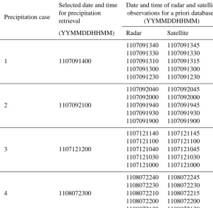
Table 1. List of precipitation cases for the precipitation estimations from the geostationary satellite and construction of a priori databases.
Precipitation case
Selected date and time Date and time of radar and satellite for precipitation observations for a priori databases
retrieval (YYMMDDHHMM)
(YYMMDDHHMM) Radar Satellite
1107091340 1107091345 1107091330 1107091330
1 1107091400 1107091310 1107091315
1107091300 1107091300 1107091230 1107091230
1107092040 1107092045 1107092000 1107092000
2 1107092100 1107091940 1107091945
1107091930 1107091930 1107091900 1107091900
1107121140 1107121145 1107121100 1107121100
3 1107121200 1107121040 1107121045
1107121030 1107121030 1107121000 1107121000
1108072240 1108072245 1108072230 1108072230
4 1108072300 1108072210 1108072215
1108072200 1108072200 1108072130 1108072130
utilizing the adjacent radar estimated precipitation and satel-lite estimations.
Some researchers have attempted to produce precipita-tion informaprecipita-tion using multi-sensor estimated precipitaprecipita-tion. Kondragunta et al. (2005) integrated the satellite precipita-tion estimates after local bias correcprecipita-tion with radar and rain gauge data in order to fill missing radar observations. Ma-hani and Khanbilvardi (2009) generated multi-sensor pre-cipitation products by merging satellite prepre-cipitation esti-mates from the Hydro-Estimator (HE) algorithm (Scofield and Kuligowski, 2003) with ground-based radar observations in order to improve satellite-based precipitation retrieval. Their results showed that merged precipitation tends to be more accurate than satellite only driven precipitation over radar gap areas. A similar approach was performed by Tesfa-giorgis et al. (2011a). The approach applied bias correction to the satellite precipitation estimates obtained from the HE algorithm and proposed a successive correction method in order to merge the satellite precipitation estimates with the radar observation.
In this study, we developed a method of precipitation esti-mation over radar gap areas based on the merging of geosta-tionary satellite and radar observations currently operated by the Korea Meteorological Administration (KMA). We used a geostationary satellite called the Communication, Ocean, and Meteorological Satellite (COMS) which was launched
in June 2010. COMS has four IR channels and one visible channel with band centers located at 3.7, 6.7, 10.8, 12.0, and 0.67 µm, respectively (Choi et al., 2007). COMS provides the brightness temperature (Tb) from IR channels every 15 min, which has a 4 km spatial resolution over the Korean Penin-sula. Precipitation estimates using IRTbfrom geostationary satellites have been presented in previous studies (e.g., Vi-cente et al., 1998; Scofield and Kuligowski, 2003). In this study, we independently estimated precipitation from COMS based on a reference of radar observations. The methodology for estimating the precipitation from a geostationary satellite and the merging technique of radar and satellite precipitation estimates are described in Sect. 2. This method was tested with four precipitation cases during the summer of 2011 (Ta-ble 1). The results of the merged precipitations are presented in Sect. 3. A summary of our study is presented in Sect. 4.
2 Methodology
Figure 1. A flow diagram to estimate the precipitation over a radar
gap area by merging the radar and satellite data.
satellite precipitation based on an a priori database. The other part (Block 2) illustrates the procedure for merging satel-lite precipitation estimates and adjacent radar observations with optimally determined weights based on reference mea-surements. The details of the methodology are discussed in the following sub-sections. Among the 11 Doppler weather radars currently operated by KMA over the Korean sula, the radar at Jindo, in the west part of the Korean Penin-sula (Fig. 2), was used in this study. The Jindo radar uses the S-band typical for weather radars with an observation range of 240 km radius. It primarily monitors precipitation and storms approaching from the west of the Korean Penin-sula.
2.1 Satellite precipitation estimation 2.1.1 The databases
Precipitation estimations from satellites in this study were principally based on the relationships between the rain rate and the satellite-observed Tb characterized by a pri-ori databases. In the construction of the a pripri-ori database, the radar-estimated rain rates were collected to ensure con-sistency with the radar. Then, the brightness temperatures at the four channels (3.7, 6.7, 10.8, and 12 µm) of COMS were collocated temporally and spatially with the radar rain rate observations in the databases. Downscaling of the satel-lite data to 1 km was performed in order to collocate the
Figure 2. The location of the Jindo radar (red triangle) and its
ob-servational coverage (black circle), which indicates the study area.
radar and satellite data, because of the difference between the radar (1×1 km) and satellite (4×4 km) spatial resolutions. A satellite pixel was split into 4 pixels in both the longitu-dinal and latitulongitu-dinal directions. Then, the collocated satellite brightness temperature (Tbcol) was computed as follows:
Tbcol= n
P
i=1
Wi·Tborg n
P
i=1 Wi
(1)
and Wi=exp
−
r2 2·resradar
, (2)
whereTborg, resradar, andrindicate theTbat the original
res-olution (4×4 km), the radar spatial resolution (1 km), and the distance between the satellite sub-pixel and radar pixel at locationi. This collocation method applies to theTbat each of the four channels. After collocation, the radar rain rate and corresponding satelliteTbwas collected over the radar obser-vational area for each of the selected precipitation cases. The databases also included non-raining areas of theTbin order to discriminate non-raining areas.
722 Y.-R. Lee et al.: Precipitation estimation over radar gap areas
Therefore, the final database consisted of sub-databases con-structed at five different time steps before the selected re-trieval period. The data and time of the radar and satellite data for each of the precipitation cases used in the construc-tion of the a priori databases are shown in Table 1. In ad-dition, each sub-database was set to have a different weight based on the time difference from the designated retrieval. The weight was expressed as follows:
Ti=exp
−t
i
tmax
, (3)
whereti is the interval between the construction time of the
ith sub-database and the designated retrieval time, andtmax is the largest time interval between the sub-databases and the retrieval. Since the radar and satellite data were avail-able every 10 and 15 min, respectively, there was a tempo-ral mismatch of 5 min between the two data sets. In order to minimize the effects of the temporal inconsistency, the mis-matched data set was assigned to have a smaller weight than the matched one.
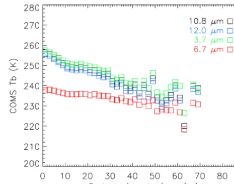
As an example of the database characteristics, the rela-tionships between the radar rain rate and the satelliteTbat the four different channels for the precipitation case 2 are shown in Fig. 3. Empty squares indicate a mean of the Tb of a 2 mm h−1interval of the radar rain rate. It was observed that theTbtended to decrease as the radar rain rate increased. Similar relationships for GOES-8Tbat 10.7 µm and the radar rain rate were also shown by Vicente et al. (1998).
2.1.2 Retrievals and bias correction
Once the a priori databases were constructed, the satellite precipitation estimation was achieved through the Bayesian inversion method as utilized by Shin and Kummerow (2003). In this approach, finding the posterior probability was the pri-mary objective. The probability may be written as follows: P (R|Tb)=P (R)×P (Tb|R), (4) where P (R|Tb) is the probability of a particular rain rate R at a givenTb,P (R)is the probability that a specific rain rate can be observed, andP(Tb|R) is the probability of ob-servingTbat a particularR. As outlined by Rodgers (2000), the conditional probability P(Tb|R) may be simulated by a multi-dimensional Gaussian distribution of the difference between the observation and the corresponding simulation from a forward model. The uncertainty was also involved in the observation and forward simulation. However, in a re-trieval using the observational database as in this study, the error from the forward computations would not appear in the covariance matrix for the termP(Tb|R). The covariance ma-trix has only the diagonal elements of the instrumental noises at each channel. Furthermore, since theP (R)of the prior in-formation, constructed during the period close to the desig-nated retrieval time, was a good description of the true prob-ability distribution of the precipitation fields observed by the
Figure 3. Mean relationship between the COMS brightness
tem-perature (Tb) and the Jindo radar rain rate. Channels at 10.8, 12.0, 3.7, and 6.7 µm are indicated by black, blue, green, and red squares, respectively.
radar, theP (R)was simply replaced by the frequency of each element in the prior information.
Figure 4. Images of the Jindo radar rain rates (left column) and
satellite precipitation estimates after bias correction (right column) for the four precipitation cases.
2.2 Merging radar and satellite precipitation estimates Precipitation estimation over radar gap areas was based on the merging of two precipitation fields: the bias-corrected satellite precipitation and the radar observations interpolated from the surrounding radar observations. The procedure to obtain the satellite precipitation estimates with bias correc-tion was discussed in the previous seccorrec-tion. The interpolacorrec-tion of the adjacent radar observations across the gap areas was performed using the following equation:
Figure 5. Scatter density diagrams of the radar rain rate
estima-tion and satellite estimated precipitaestima-tion after bias correcestima-tion for the four precipitation cases of (a) case 1, (b) case 2, (c) case 3, and
(d) case 4. Comparison statistics including correlation coefficient
(Corr), bias, and root-mean-square error (RMSE) are also presented in each panel.
R0=
N
P
k=1 Ik·Rk
N
P
k=1 Ik
, (5)
whereR0 is the interpolated radar rain rate at a pixel at the radar resolution over the gap area andRk is the radar
ob-served rain rate at the kth pixel among N pixels within a 5 km distance from the location ofR0.Ik is the kth pixel’s
weight determined by the following Gaussian function:
Ik=exp
−dk2
2r2
!
, (6)
wheredk is the distance (km) between the given pixel over
724 Y.-R. Lee et al.: Precipitation estimation over radar gap areas
merging was applied only within the gap area, so that the initial radar observations remained intact outside of the gap area.
In order to generate the merged precipitation field, the weight coefficients allocating the contribution from each data set over the radar gap area needed to be determined. The weight coefficients are calculated at each pixel. The pro-posed method in this study is thus considered a successive correction implying a pixel-by-pixel calculation of the gap (e.g., Brandes, 1975; Mahani and Khanbilvardi, 2009; Tesfa-giorgis and Mahani, 2013). The previous study of Bran-des (1975) applied a successive correction method to produce radar calibration fields using rain gauges. Mahani and Khan-bilvardi (2009) and Tesfagiorgis and Mahani (2013) used satellite precipitation estimates and surrounding radar pre-cipitation within a moving window. These studies utilized the difference between radar and satellite precipitation estima-tions of surrounding gap (outside of the gap) for generating merged precipitation. This study first estimates satellite pre-cipitation and interpolates the radar rain rate field over the gap areas using surrounding radar-estimated precipitation. Optimal merging weights are then determined for the satel-lite precipitation and interpolated precipitation fields based on the RMSE difference from the reference data. The weight coefficient,Kl, for thelth data set can be written as follows:
Kl= 1 σl2 n
P
m=1 1 σ2 m
l=1, . . ., n, (7)
whereσlandσmare the RMSE difference from the reference
data for the lth andmth data sets, respectively. In order to evaluate the accuracy of the merged precipitation field, the synthetic radar gap areas in the radar observational coverage were set and three experiments with the two different refer-ence data sets and the equal weight were performed.
The first determined the optimal weights based on the orig-inal radar observation over the synthetic gap area. This ex-periment was not possible in practice, since the radar obser-vations did not exist over the gap area. It was deliberately performed in order to compare with the other two merg-ing experiments. The second experiment used the Automatic Weather Station (AWS) data as the reference observation. The AWS observation nearest to the merging pixel was se-lected in this experiment. The final one assigned equal weight coefficients to each data set (Kl=1/n). The weight
coeffi-cient was 1/2 for the two data sets. This experiment could be used in case any reference data were not available over the gap area. The merging method works for either of the rain or no-rain cases over the gap areas. The results of the three ex-periments merging the interpolated radar precipitation field and bias-corrected satellite precipitation data over the radar gap area are presented in the next section. In the experiments, the radar gap areas were selected over significant raining re-gions with rain rates greater than 10 mm h−1and its size was
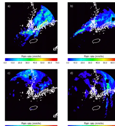
Figure 6. Images of the Jindo radar rain rate estimations for the four
different precipitation cases of (a) case 1, (b) case 2, (c) case 3, and
(d) case 4. The black boxes in the rain images indicate the synthetic
radar gap areas whose size is 0.3◦×0.3◦latitude-longitude.
set to 0.3◦×0.3◦latitude-longitude. The images for the four radar observation cases with the synthetically located gap ar-eas (black box) are shown in Fig. 6.
3 Result and discussions
Figure 7. Precipitation distributions estimated by the Jindo radar
for the four precipitation cases (the first column), same as in Fig. 6, but focused on the surrounding of the gap areas (black line box). Precipitation estimations over the black boxes from the three merg-ing experiments employmerg-ing the optimal weights determined by the original radar data and the AWS data, and the equal weights (1/2) are illustrated in the rest of the columns, respectively.
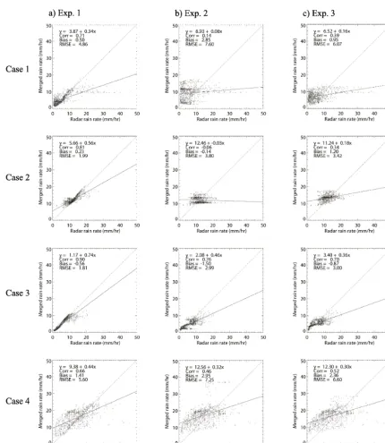
Figure 8 also compares the accuracy of the three merging experiments for each of the precipitation cases. The first ex-periment (column Exp. 1) appeared to produce higher qual-ity precipitation estimates over the gap areas with high cor-relations (0.71, 0.81, 0.90, and 0.66) and relatively low bi-ases (−0.50, 0.23,−0.56, and 1.41) for the four precipitation cases. This result may have been expected, because the origi-nal radar observations over the gap areas were involved in the merging process. On the other hand, the other merging meth-ods (Exps. 2 and 3) did not appear to produce comparable results relative to the first experiment. In addition, the vary-ing estimation statistics may suggest that the accuracy of the merged results tended to depend on the precipitation cases and the location of the gap areas. In particular, the correlation coefficients from the second experiment based on the AWS data turned out to be highly variable ranging from−0.06 to 0.76.
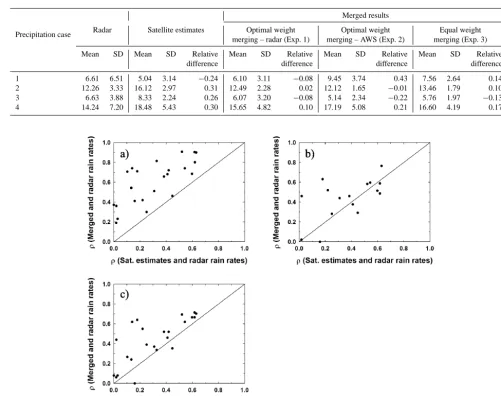
Comparisons of the radar observations, satellite estimates, and merged results for their mean and standard deviations are also presented in Table 2. In this study, the relative difference was the ratio of the difference between the mean satellite esti-mate (or the mean merged estiesti-mate) and the mean radar rain
rate to the mean radar rain rate. The standard deviations of the merged results were less than those of the radar observa-tions for all of the precipitation, implying that the variability of the merged precipitation field was smaller than that of the radar observation. For example, as shown in Table 2, the rela-tive differences for the three merging experiments were quite small (0.02,−0.01, and 0.10 mm h−1) for the precipitation case 2, while the standard deviation differences between the radar and merged precipitations were still noticeable. This result suggests that the smaller variability appeared to be a characteristic of the merged precipitation field and made a distinct discontinuity around the gap areas in case 2 (Fig. 7), regardless of the small relative differences. The other high-light was that the absolute relative differences of the merged results were smaller than those of the satellite estimates in most of the cases. This indicates that the merging methods tended to lead to better agreement with the radar observation than applying only the satellite precipitation estimates to the radar gap areas.
An attempt was made to analyze the impacts of the satel-lite precipitation estimates on the merged results with addi-tional radar gap areas at different locations and two differ-ent precipitation cases including 10 July 2011, 12:00 (lo-cal time) and 7 August 2011, 16:00. Figure 9 shows the scatter diagrams of two of the correlation coefficients. The first correlation (ρsr) was obtained from the satellite esti-mates and the radar observations. The second (ρmr) indi-cated the relationship between the merged precipitation es-timates and the radar observation. Each of the scatter dia-grams represents one of the three merging methods: (a) opti-mal weight using radar, (b) optiopti-mal weight using AWS, and (c) equal weight. An increasing trend ofρmrwith an increase inρsrexisted, indicating that highly correlated satellite pre-cipitation estimates with radar observations produced well matched merged precipitation fields over the radar gap with radar observation, especially with merging methods of op-timal weight using radar and equal weight. In other words, more accurate precipitation estimation from satellites created better merged results. This indicates that the accuracy of the merged results depended on the accuracy of the satellite pre-cipitation estimates. It was also obvious thatρmr was typi-cally larger thanρsr except for a few cases in the merging with AWS and equal weight. This result implies that using merged precipitation fields helped to estimate more accu-rate precipitation than using only satellite precipitation es-timation over the radar gap area. In addition, the optimal weight merging using the AWS method showed less depen-dence on satellite estimates. This result may have been due to the sparse distribution of the AWS observation data, which failed to resemble the spatial characteristics of the radar ob-servation.
726 Y.-R. Lee et al.: Precipitation estimation over radar gap areas
Figure 8. Scatter diagrams for the radar rain rate estimations vs. the merged precipitation over the radar gap areas using the merging methods
of (a) optimal weight using radar, (b) optimal weight using AWS, and (c) equal weight for each of the precipitation cases.
merging method produced better merged results than the op-timal weight merging using AWS. This result suggests that the optimal weight information from the AWS appeared to be inaccurate. The reason for this inaccuracy, as we have dis-cussed previously, may be that the distance between the gap pixel and the AWS (maximum 5 km) did not guarantee an accurate description of the spatial characteristics of the radar observation.
4 Summary
Table 2. Mean (mm h−1) and standard deviation (SD) (mm h−1) values of the radar observation, satellite precipitation estimates after bias correction, and radar-satellite merged results over the radar gap areas for the four precipitation cases. In this study, the relative difference indicates the ratio of the difference between the satellite estimates or merged results from the radar observation to the mean radar observation over the radar gap area.
Precipitation case
Merged results
Radar Satellite estimates Optimal weight Optimal weight Equal weight
merging – radar (Exp. 1) merging – AWS (Exp. 2) merging (Exp. 3)
Mean SD Mean SD Relative Mean SD Relative Mean SD Relative Mean SD Relative
difference difference difference difference
1 6.61 6.51 5.04 3.14 −0.24 6.10 3.11 −0.08 9.45 3.74 0.43 7.56 2.64 0.14
2 12.26 3.33 16.12 2.97 0.31 12.49 2.28 0.02 12.12 1.65 −0.01 13.46 1.79 0.10
3 6.63 3.88 8.33 2.24 0.26 6.07 3.20 −0.08 5.14 2.34 −0.22 5.76 1.97 −0.13
4 14.24 7.20 18.48 5.43 0.30 15.65 4.82 0.10 17.19 5.08 0.21 16.60 4.19 0.17
Figure 9. Scatter diagrams of the two correlation coefficients. The first correlation in the abscissa is obtained from the satellite estimates and
radar rain rate estimations. The other correlation in the ordinate is from the merged precipitation estimates and the radar rain rate estimations. Panels are classified by the three merged precipitation estimates from (a) optimal weight using radar, (b) optimal weight using AWS, and (c) equal weight.
relationships between the radar rain rate and the satelliteTb in the database. The initial satellite estimates were then ad-justed by an ensemble bias correction method (Tesfagiorgis et al., 2011b) using the radar data.
The merging of the bias-corrected satellite precipitation and interpolated radar precipitation fields over the radar gap areas was implemented by optimal weight merging. The weights were calculated optimally from the radar and AWS. For comparison, an additional merging experiment with equal weight was included.
728 Y.-R. Lee et al.: Precipitation estimation over radar gap areas
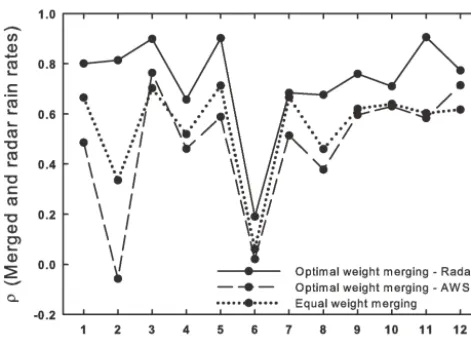
Figure 10. The correlation coefficients between the merged
precip-itation and radar rain rate estimation over the different gap areas. The merged precipitation estimates are obtained from the merging methods of optimal weight using radar (solid line), optimal weight using AWS (dashed line), and equal weight (dotted line).
the radar gap area, with variable correlation coefficients of 0.34–0.70 depending on the precipitation cases (Fig. 8). The results of this experiment may be used to produce practical precipitation estimates when any other ground observation is not available. In terms of the mean value of precipitation over the gap areas, the merged precipitation field agreed with the original radar data within∼17 % except for one method of merging (Table 2). More importantly, the results of this study demonstrate that more accurate precipitation estimation from satellites is essential in order to create better merging results over the radar gap areas (Fig. 9).
Acknowledgements. This research was supported by the “De-velopment and application of cross governmental dual-pol radar harmonization (WRC-2013-A-1)” project of the Weather Radar Center, Korea Meteorological Administration in 2014.
Edited by: M. Portabella
References
Austin, P. M.: Relation between measured radar reflectivity and sur-face rainfall, Mon. Weather Rev., 115, 1053–1070, 1987. Brandes, E. A.: Optimizing rainfall estimates with the aid of radar,
J. Appl. Meteor., 14, 1339–1345, 1975.
Choi, Y.-S., Ho, C.-H., Ahn, M.-H., and Kim, Y.-M.: An exploratory study of cloud remote sensing capabilities of the Communica-tion, Ocean and Meteorological Satellite (COMS) imagery, Int. J. Remote Sens., 28, 4715–4732, 2007.
Kidd, C., Kniveton, D. R., Todd, M. C., and Bellerby, T. J.: Satel-lite rainfall estimation using combined passive microwave and infrared algorithms, J. Hydrometeor., 4, 1088–1104, 2003. Kondragunta, C., Kitzmiller, D., Seo, D. J., and Shrestha, K.:
Objec-tive integration of satellite, rain gauge, and radar precipitation es-timates in the multisensor precipitation estimator algorithm, 19th Conference on Hydrology, San Diego, CA, Amer. Meteor. Soc., 2005.
Mahani, S. E. and Khanbilvardi, R.: Generating multi-sensor pre-cipitation estimates over radar gap areas, WSEAS Transactions on Systems, 8, 96–106, 2009.
Rodgers, C. D.: Inverse Methods for Atmospheric Sounding: The-ory and Practice, World Scientific, Singapore, 2000.
Scofield, R. A. and Kuligowski, R. J.: Status and outlook of opera-tional satellite precipitation algorithms for extreme-precipitation events, Weather Forecast., 18, 1037–1051, 2003.
Shin, D.-B. and Kummerow, C.: Parametric rainfall retrieval algo-rithms for passive microwave radiometers, J. Appl. Meteorol., 42, 1480–1496, 2003.
Tesfagiorgis, K. and Mahani, S. E.: A multi-source precipitation es-timation approach to fill gaps over a radar precipitation field: a case study in the Colorado River Basin, Hydrol. Process., 29, 29–42, doi:10.1002/hyp.10103, 2013.
Tesfagiorgis, K., Mahani, S. E., and Khanbilvardi, R.: Multi-sources precipitation estimation: Mitigating gaps over radar network cov-erage, in: Proceedings of IGARSS, Vancouver, BC, 3054–3056, 2011a.
Tesfagiorgis, K., Mahani, S. E., Krakauer, N. Y., and Khanbil-vardi, R.: Bias correction of satellite rainfall estimates using a radar-gauge product – a case study in Oklahoma (USA), Hy-drol. Earth Syst. Sci., 15, 2631–2647, doi:10.5194/hess-15-2631-2011, 2011b.