www.ocean-sci.net/5/403/2009/
© Author(s) 2009. This work is distributed under the Creative Commons Attribution 3.0 License.
Ocean Science
Controlling atmospheric forcing parameters of global ocean models:
sequential assimilation of sea surface Mercator-Ocean reanalysis
data
C. Skandrani1, J.-M. Brankart1, N. Ferry2, J. Verron1, P. Brasseur1, and B. Barnier1 1Laboratoire des Ecoulements G´eophysiques et Industriels (LEGI/CNRS), Grenoble, France 2Mercator-Oc´ean, Toulouse, France
Received: 26 May 2009 – Published in Ocean Sci. Discuss.: 18 June 2009
Revised: 17 September 2009 – Accepted: 21 September 2009 – Published: 16 October 2009
Abstract. In the context of stand alone ocean models, the at-mospheric forcing is generally computed using atat-mospheric parameters that are derived from atmospheric reanalysis data and/or satellite products. With such a forcing, the sea surface temperature that is simulated by the ocean model is usually significantly less accurate than the synoptic maps that can be obtained from the satellite observations. This not only penalizes the realism of the ocean long-term simulations, but also the accuracy of the reanalyses or the usefulness of the short-term operational forecasts (which are key GODAE and MERSEA objectives). In order to improve the situation, partly resulting from inaccuracies in the atmospheric forc-ing parameters, the purpose of this paper is to investigate a way of further adjusting the state of the atmosphere (within appropriate error bars), so that an explicit ocean model can produce a sea surface temperature that better fits the available observations. This is done by performing idealized assimila-tion experiments in which Mercator-Ocean reanalysis data are considered as a reference simulation describing the true state of the ocean. Synthetic observation datasets for sea sur-face temperature and salinity are extracted from the reanaly-sis to be assimilated in a low resolution global ocean model. The results of these experiments show that it is possible to compute piecewise constant parameter corrections, with pre-defined amplitude limitations, so that long-term free model simulations become much closer to the reanalysis data, with misfit variance typically divided by a factor 3. These results are obtained by applying a Monte Carlo method to simu-late the joint parameter/state prior probability distribution. A truncated Gaussian assumption is used to avoid the most
ex-Correspondence to: J.-M. Brankart
(jean-michel.brankart@hmg.inpg.fr)
treme and non-physical parameter corrections. The general lesson of our experiments is indeed that a careful specifica-tion of the prior informaspecifica-tion on the parameters and on their associated uncertainties is a key element in the computation of realistic parameter estimates, especially if the system is affected by other potential sources of model errors.
1 Introduction
models are used to simulate the ocean component alone, the control of the atmospheric parameters using ocean surface observations is certainly an appropriate way of improving the realism of model interannual simulations, the accuracy of ocean reanalyses or the usefulness of sea surface temper-ature operational forecasts. It is thus also an important con-tribution to the GODAE1objectives (GODAE, 2008), which is the reason why a large part of the MERSEA2effort in the development of data assimilation has been devoted to this problem.
In this study, which has been conducted as part of the MERSEA project, this problem is investigated using ideal-ized experiments in which Mercator-Ocean3ocean reanaly-sis data are used as the reference simulation (i.e. the “truth” of the problem). Synthetic observation datasets (for sea sur-face temperature and sea sursur-face salinity) are extracted from the reanalysis to be assimilated in a coarse resolution global ocean model. With respect to Skachko et al. (2009), who investigated a similar problem using twin assimilation exper-iments, the present study is thus more realistic, since the dif-ference between model and reanalysis is now very similar in nature to the real error. It is closer to the real problem even if the experiments are still somewhat ideal in the sense that no real observations are assimilated, and that the full reference model state (the reanalysis, in three dimensions) is available for validation. Another difference with respect to Skachko et al. (2009) is that, in this paper, we extend the control vector to 6 atmospheric parameters instead of 2 turbulent exchange coefficients in their example (but we exclusively focus on the control of the parameters, while they also considered the joint optimal estimate of the ocean state vector together with the atmospheric parameters). However, in order to solve this more realistic problem, we needed to further develop the methodology towards a better specification of the prior infor-mation about the parameters and their associated uncertainty. We observe indeed that making appropriate assumptions on that respect is increasingly important as the estimation prob-lem is becoming more realistic, because it is more and more difficult to make the distinction between forcing errors and the other potential sources of error in the system. An addi-tional important objective is thus to find means of identifying properly the part of the observational misfit that can be inter-preted as resulting from inaccurate atmospheric parameters.
In order to reach this objective, the plan is to apply se-quentially a Bayesian inference method to compute piece-wise constant optimal parameter corrections. A possible al-gorithm to solve this problem is to compute the optimal pa-rameters by direct maximization of the posterior probability distribution for the parameters, using for instance a 4DVAR scheme (as done in Roquet et al., 1993 or Stammer et al., 2004). But, in addition to the technical difficulties that the
1http://www.godae.org
2http://www.mersea.eu.org
3http://www.mercator-ocean.fr
algorithm may involve, this solution requires that the cost function resulting from the optimal probabilistic criterion be quadratic or at least differentiable everywhere in parameter space, so that it is by no way straightforward to optimally im-pose strict inequality constraints to the parameters (by setting zero prior probability in prohibited region of the parameter space for instance). This is why, in this study, we prefer using a Monte Carlo algorithm to simulate the ocean response to parameter uncertainty, and use the resulting ensemble repre-sentation of the prior probability distribution to infer optimal parameter corrections from the ocean surface observations. It is in the specification of this prior probability distribution that two methodological improvements are introduced with respect to Skachko et al. (2009). First, the error statistics are computed locally in time for each assimilation cycle, by performing a sequence of ensemble forecasts around the cur-rent state of the system (while they are assumed constant in their study). And second, the probability distribution is as-sumed to be a truncated Gaussian distribution (as proposed by Lauvernet et al., 2009, as an improvement to the classi-cal Gaussian hypothesis), in order to avoid the most extreme and non-physical parameter corrections. These two improve-ments are indeed found necessary to solve the more realistic assimilation problem at stake in this paper.
However, before explaining this in more detail, we first summarize in Sect. 2 the background existing elements that are used to perform the study: the ocean model, the assim-ilation method for parameter estimation and the Mercator-Ocean reanalysis data. Then, in Sect. 3, we present the de-tails of the method that is used to perform the assimilation experiments: experimental setup and statistical parameteri-zation. And finally, in Sect. 4, we discuss and interpret the results, focusing on the accuracy of the mixed layer thermo-haline characteristics and on the relevance of the parameter estimates.
2 Background
In this section, we present the three existing ingredients that are used later as a background information to set up our as-similation system (Sect. 3) and to perform the experiments (Sect. 4): (i) the ocean model, focusing on the role of the at-mospheric forcing parameters, (ii) the assimilation method, in order to introduce the various approximations and param-eterizations that are needed to solve the problem, and (iii) the Mercator-Ocean reanalysis, from which the synthetic obser-vations are extracted.
2.1 Ocean model
in order to improve the representation of the equatorial dy-namics. This is a free surface configuration based on the resolution of primitive equations, with a z-coordinate ver-tical discretization. There are 31 levels along the verver-tical, and the vertical resolution varies from 10 m in the first 120 m to 500 m at the bottom. The lateral mixing for active trac-ers (temperature and salinity) is parameterized along isopy-cnal surfaces, and the model uses a turbulent kinetic energy (TKE) closure scheme to evaluate the vertical mixing of mo-mentum and tracers (Blanke and Delecluse, 1993).
The model is forced at the surface boundary with heat, freshwater and momentum fluxes. The fluxes through the ocean surface are estimated from the atmospheric parame-ters at the anemometric height, using the bulk semi-empirical aerodynamic formulas. Daily atmospheric variables (wind, humidity, air temperature, cloud coverage) from NCEP and monthly mean precipitation from CMAP (CPC Merged Analysis of Precipitation) are used to interactively diagnose the net heat and fresh water fluxes (QNET and F WNET),
which can be written respectively:
QNET=QS+QL+QLW+QSW (1)
F WNET=E−P −R (2)
whereQS is the sensible heat flux,QLthe latent heat flux,
QLWthe long wave radiation flux,QSWthe short wave solar
radiation flux, andE,P,Rare the three terms related to the fresh water budget, respectively evaporation, precipitations and river runoffs. The flux parameters which are involved in the computation of these quantities are the latent heat flux coefficient (CE), the sensible heat flux coefficient (CH), sea
surface temperature (Tw), air temperature (Ta), air pressure,
atmospheric specific humidity (qa), wind speed (W10), cloud
coverage (C) and precipitation (P). For more detail on these bulk formulas, the reader can refer to the CLIO (Coupled Large-scale Ice Ocean) model description in Goosse et al. (1999).
The turbulent latent and sensible heat fluxes are calcu-lated from the classical ocean-atmosphere transfer equations (Large and Pond, 1982):
– the latent heat flux:
QL=ρaLeCEW10max(0, qs−qa) (3)
whereρa is the air density, Le the vaporization latent
heat, andqsthe saturation specific humidity; – the evaporation fresh water flux :
E=QL/Le (4)
– the sensible heat flux:
QS =ρacapCHW10(Tw−Ta) (5)
wherecpais the air specific heat;
– the long-wave radiation flux, which is parameterized by following Berliand and Berliand (1952):
QLW=σsbTa4(0.39−0.05
√
ea)(1−χ C2)+4σsbTa3
(Tw−Ta) (6)
whereea (in mb) is the vapor pressure deduced from
qa,, the surface emissivity,σsbthe Stephan-Boltzmann
constant,(1−χ C2), a correction factor to take into ac-count the effect of clouds;
– the short-wave radiation flux, following the proposed formula by Zillmann (1972):
QSW=(1−α)(1−0.62C+0.0019β)QCLEAR (7)
whereαis the ocean albedo,β, the zenith angle at noon andQCLEAR, the solar radiation at the ocean surface in
clear weather.
For the momentum flux, we did not use aerodynamic bulk formulas to calculate the wind stress vector. It is directly specified in the model, using ERS scatterometer data com-plemented by in-situ observations of TAO derived stresses (Menkes et al., 1998). No relaxation to observed SST and SSS is applied in our simulations.
2.2 Assimilation method
The purpose of this section is to briefly describe the assim-ilation methods that are applied to perform this study. Only general algorithms and equations are given here; the spe-cific parameterizations on which they depend are presented in Sect. 3.
2.2.1 Estimation of model parameters
The problem of estimating model parameters from ocean ob-servations can be formulated using the Bayesian inference framework. From a prior probabilityp(α)for a vector of un-certain parametersα, and the conditional probability distri-butionp(y|α)for obtaining a vector of observations y given the vector of parametersα, the Bayes theorem:
In this problem, the observations y are usually not di-rectly related to the parameters α, but to the model solu-tion x that is a funcsolu-tion ofα, so that the probability distri-butionp(y|α)is usually defined as a function of the misfit between the observations and the model solution correspond-ing toα: y−Hx(α)(innovation vector), where H is the ob-servation operator. This makes the computation ofα∗more difficult, either with direct minimization techniques, because every evaluation of the function to minimize requires one model simulation (and also one adjoint model simulation if the gradient is also computed), or with Monte Carlo methods, because they require an ensemble model forecast using an ensemble of parameter vectors drawn from their prior proba-bility distribution.
In this study, Monte Carlo simulations are performed to compute the model counterpart x to an ensemble of param-eter vectors, sampled from p(α). This ensemble forecast characterizes the prior probability distributionp(xˆ)for the augmented vectorxˆ=[α,x(α)], characterizing the model re-sponse to parameter uncertainty. It is important to note that, up to this point, linearity has not been assumed, and that it is only at this stage that a Gaussian parameterization is used for the prior distributionp(xˆ), with the consequence of lin-earizing the inference rules relating the model parametersα to the observations y (see below). In order to mitigate the ef-fect of this linearization, the problem is divided in a sequence of short periods of time (assimilation cycles) and the param-etersα are estimated separately and sequentially for every element of the sequence (see Sect. 3 for more detail). 2.2.2 Optimal estimate under Gaussian assumption
If the probability distribution p(xˆ) and p(y| ˆx) can be as-sumed Gaussian:
p(xˆ)∼N(xˆb,Pˆ) and p(y| ˆx)∼N(Hˆxˆ,R) (9) wherexˆbis the background simulation,P is the backgroundˆ error covariance matrix in the augmented space,Hˆ=[0,H] is the augmented observation operator and R the observation error covariance matrix, it is known that the posterior proba-bility distributionp(xˆ|y)is also Gaussian:
p(xˆ|y)∼N(xˆa,Pˆa) (10) where the meanxˆa and the covariancePˆa are given by the standard linear observational update formulas:
ˆ
xa= ˆxb+K(y− ˆHxˆb) and Pˆa =(I−KHˆ)Pˆ with K=(HˆPˆ)T(HˆPˆHˆT +R)−1 (11) Equation (11) are also the equations of the observational update of a Kalman filter written for an augmented control vector (including model parameters in addition to the model state). This method can be applied to control other sources of error in addition to parameter error (as explained, for in-stance, in Skachko et al., 2009). However, in the present
study, Eq. (11) are only going to be used to obtain improved parameter estimates.
It is interesting to note that the solution given by Eq. (11) is not equivalent to minimizing
J (α)=1 2α
TP−1 α α+
1
2[y−Hx(α)]
TR−1[y−Hx(α)] (12)
(where Pαis the block ofP corresponding to the vector ofˆ
parameters) using a variational method, as soon as the func-tion x(α)relating the model solution to the parameters is nonlinear. This variational solution only assumes Gaussian-ity of p(α) andp(y|x)while keeping the nonlinear func-tion x(α)in the expression of
p(α|y)∼p(α)p(y|α)∼exp[−J (α)] (13) which is not Gaussian. However, there is no prerequisite of Gaussianity in Monte Carlo methods, that may also of-fer other advantages. It is for instance easier to apply strict inequality constraints (by modifying the prior Gaussian as-sumption). This possibility is exploited in this study to con-fine the parameter estimates in a predecon-fined region of the pa-rameter space (see Sect. 3.5).
2.2.3 Reduced rank approximation
If the background error covariance matrix is available in square root formPˆ= ˆSSˆT, with a rank given by the numberr
of independent columns inS (the error modes), then the prob-ˆ lem can be simplified to the estimation of a reduced vectorξ (of sizer), giving the amplitudes of the correction toxˆbalong each column ofS, using a reduced observation vectorˆ η(of sizer) resulting from the projection of the innovations onto the error modesS:ˆ
ˆ
x= ˆxb+ ˆSUξ and η=3(HˆSUˆ )TR−1(y− ˆHxˆb) (14) where U (unitary matrix) and3(diagonal matrix) are the ma-trices with eigenvectors and inverse eigenvalues of ther×r
matrix:
(HˆSˆ)TR−1(HˆSˆ)=U3−1UT (15) By transformation (14), the probability distributions (Eq. 9) transforms to
p(ξ)∼N(0,I) and p(η|ξ)∼N(ξ,3) (16) so that
p(ξ|η)∼N(ξa,3a) with ξa= [I+3]−1η and
3a= [I+3]−13 (17)
2.3 Mercator-Ocean reanalysis
Mercator-Ocean is an operational oceanography center based in Toulouse, France. It develops and runs operational ocean analysis/forecast systems specially designed to provide use-ful products for several downstream applications: research, institutional and operational applications, private sector ap-plications and environmental policy makers. Mercator-Ocean also periodically delivers ocean reanalyses, that are produced using up-to-date ocean models, observations and assimilation methods. In this study, we are using the data from a Mercator-Ocean coarse resolution global reanalysis (PSY2G2). The main application of this reanalysis is to pro-vide ocean initial conditions for coupled seasonal prediction applications (Balmaseda et al., 2008), but it is also used for research purposes as it provides a long coherent time series of the ocean state (from 1980 to present). The ocean model used in the reanalysis is similar in many points to the one that is used in our experiments: same numerical code OPA, same grid, same physics, but different atmospheric forcing, which is computed using the ERA-40 reanalysis for the pe-riod January 1979 to December 2001. The assimilated ob-servations are subsurface temperature and salinity, SLA data and SST maps. The subsurface data come from the EN-ACT/ENSEMBLES data base provided by the CORIOLIS4 data center; the altimetric data are along-track SLA (from November 1992 to present) provided by SSALTO/DUACS; and the SST maps are obtained from the Reynolds OIv2 product (Reynolds et al., 2002). The reanalysis data assim-ilation scheme is a reduced order Kalman filter using the SEEK formulation (Pham et al., 1998). The forecast error covariance is based on the statistics of a collection of 3-D ocean state anomalies (typically a few hundred) and is sea-sonally variable. The statistical analysis produces tempera-ture and salinity as well as barotropic velocity increments, from which zonal and meridional velocity fields are deduced using physical balance operators. For the present study, we extracted 1993 and 1994 data (temperature and salinity) for use in our assimilation experiments.
3 Method
3.1 Setup of the assimilation experiments
The general idea of the experiments presented in this paper is to use the Mercator-Ocean reanalysis as reference simula-tion from which synthetic observasimula-tion datasets are extracted, and to assimilate these observations into our ocean model as a constraint to the atmospheric forcing function. These ex-periments are ideal in the sense that no real observations are assimilated and that the full reference model state (in three dimensions) is available for validation. But they are also re-alistic (clearly distinct from twin experiments) because
dif-4http://www.coriolis.eu.org
ferences of model simulations with respect to the reanalysis are similar in nature to differences with respect to the real world. It is indeed expected that the assimilation of the real observations to build the reanalysis moved the model trajec-tory towards a more realistic description of the ocean. The starting date of the experiments is 30 December 1992 (with an initial condition from a standard simulation performed by Castruccio et al., 2008). The first six months are used as an initialization period for the assimilation system, so that the one year diagnostic period extends from 30 June 1993 to 29 June 1994. Figure 1 (left panel, top black line) shows the time evolution of the RMS error (difference with respect to the reanalysis) in the free simulation (i.e. without parameter corrections) for sea surface temperature (SST) and sea sur-face salinity (SSS), as computed over the world ocean south of 70◦N, to avoid some problematic ice covered regions. We can observe on the figure that the SST RMS error is stable in time (in the interval 0.85–1.05◦C) but that the SSS RMS er-ror is drifting from the beginning of the simulation (at a rate of about 0.1 psu per year).
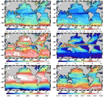
The error is however very inhomogeneous horizontally, as can be seen in Fig. 2, showing maps of SST and SSS sys-tematic error (top panels) and maps of SST and SSS error standard deviations (bottom panels), averaged over the one year diagnostic period. The largest systematic errors (up to 2◦C and 0.8 psu) or error standard deviation (up to 1.5◦C and 1 psu) are localized in the regions of the Western bound-ary currents and the Antarctic Circumpolar Current (ACC). These large errors are due to the poor representation and localization of the ACC and the boundary currents in our low resolution ocean model. Since these currents are asso-ciated to the most intense SST and SSS fronts in the ocean, it is mostly the misplacement of the currents that leads to the largest SST and SSS errors. In these regions, the atmo-spheric forcing function is not the dominant cause of error, so that the identification of forcing errors is almost impossible there (with a low resolution model). This is why they will be masked in several diagnostics involving horizontal averages. The right panel of Fig. 1, for instance, shows the same re-sult as the left panel as obtained by masking the 10% of the ocean with the largest free run RMS misfit. The mask is thus different for SST and SSS, and can be visualized in Fig. 2, as the region with the largest misfit (i.e. essentially the Western boundary currents and a part of the ACC). The RMS error for this 90% subdomain remains quite large in the free sim-ulation with a reduction of about 10% for SST and 30% for SSS with respect to the global RMS error.
J F M AM J J A S O N DJ M AM J J1993F M AM J J A S O N DJ1994FM AM J
J1993F M AM J J A S O N DJ1994FM AM J J1993F M AM J J A S O N DJ1994FM AM J
1993 1994
F
Fig. 1. Misfits between the simulations and the SST (top panels) or SSS (bottom panels) observations for the
world ocean (south of 70◦N) as computed, without masking any regions (left panels) or by masking the 10% of the ocean surface that is charcterized by the largest free run RMS misfit (right panels). The figures show the free simulation (upper black solid line), the relaxation towards a perfect initial condition (dashed black line), the modified free simulation starting from this perfect initial condition (lower black solid line), the simulation with parameter optimization (green line), the simulation with parameter optimization starting from perfect initial condition (red line). The vertical dashed-dotted line marks the beginning of the one year diagnostic period.
24
Fig. 1. Misfits between the simulations and the SST (top panels) or SSS (bottom panels) observations for the world ocean (south of 70◦N) as computed, without masking any regions (left panels) or by masking the 10% of the ocean surface that is charcterized by the largest free run RMS misfit (right panels). The figures show the free simulation (upper black solid line), the relaxation towards a perfect initial condition (dashed black line), the modified free simulation starting from this perfect initial condition (lower black solid line), the simulation with parameter optimization (green line), the simulation with parameter optimization starting from perfect initial condition (red line). The vertical dashed-dotted line marks the beginning of the one year diagnostic period.
forcing parameters using a sequential assimilation method. The simulation is thus divided in a sequence of time inter-vals (the assimilation cycles, with a length of 7 days), for which we estimate the forcing parameters by combining op-timally forcing prior knowledge and available ocean obser-vations. In our experiments, the forcing parameter estimates are obtained using SST and SSS observations extracted from the reanalysis at the model resolution with global coverage and perfect accuracy.
3.2 Initial condition
In such a kind of experiment, an important difficulty occurs if we start the assimilation experiment from the initial condi-tion of the free model simulacondi-tion on 1 January 1993, because at the end of the first one-week assimilation cycle, most of the error (difference with respect to reanalysis) is due to ini-tial condition error and not to errors in the atmospheric forc-ing (correspondforc-ing to this first cycle). To avoid this difficulty, we first present results that are obtained without initial con-dition error. In that way, a better view of the behaviour of the method can be produced, thus facilitating the interpretation of the results. The influence of initial condition error is only briefly considered in a second stage.
In order to build a perfect initial condition for the assim-ilation experiments, we simply perform an ideal assimila-tion experiment with perfect incrementδxk, computed as the
difference between the model forecast of the current cycle (numberk) and the corresponding ocean state in the reanal-ysis. This increment is then introduced into the model using the incremental analysis update algorithm (as in Ourmi`eres et al., 2006). Moreover, in order to distribute the effort over the firstp assimilation cycles, this increment is divided by the factor max(p−k+1,1). In that way, only onepth of the full increment is applied during the first cycle, and the cycle p is the first cycle with the full perfect increment. Figure 1 (left panel, dashed black line) shows the SST and SSS RMS error reduction during this initialization procedure from 30 December 1992 to 10 March 1993 (10 cycles of 7 days withp=8). This last date is the initial condition of our simplified assimilation experiments (with negligible ini-tial condition error). For comparison purpose, a free model simulation starting from this perfect initial condition is also presented in Fig. 1 (lower black solid line), showing that the corresponding SST and SSS misfits quickly increase with time to reach asymptotically the typical misfit (for SST) or the typical trend (for SSS) that is observed in our original free model simulation (with wrong initial conditions). 3.3 Forcing parameters prior probability distribution
As explained in Sect. 2.2, the estimation of model param-eters using Bayesian inference requires the definition of a prior probability distribution for the parameters. And the first thing to decide about this probability distribution is the list of
uncertain parameters to include in the control vector (step a in Table 1); other parameters are then considered perfectly accurate. In this study, we decide to estimate the follow-ing parameters of the atmospheric forcfollow-ing function: air tem-perature (Ta), air relative humidity (qa), cloud fraction (C),
precipitation (P), the latent heat flux coefficient (CE) and the
sensible heat flux coefficient (CH). The reason for this choice
is that they are expected to be the most important inaccurate parameters that are involved in the computation of the net heat and fresh water fluxes at the air-sea interface. They are assumed to be responsible for most of the error in the com-putation of these net fluxes, and thus to be one of the most important source of error in the heat and salt budget of the ocean mixed layer. One important missing parameter is wind velocity, which is a key parameter to control the heat flux computation (Mourre et al., 2008). The reason for which it is not included in the list of control parameters is that it is also correlated to the momentum flux (zonal and meridional wind stress components), which we have chosen not to control in this study. The decision not to control this important source of model error results from the necessity of proceeding step by step to avoid unpredictable difficulties in the solution of the inverse problem. However, we must be aware that, as any uncontrolled error (like the localization of the boundary currents), this can introduce compensation problems in the parameter estimates (see Sect. 4.3).
In order to define the prior probability distribution for these control parameters (step b in Table 1), we first as-sume that the error on the parameters is constant over the current assimilation cycle, which already means that the overal flux correction in our experiments is necessarily piece-wise constant (with weekly forcing parameter increments). Second, we assume that the parameter error pdf is Gaus-sianN(0,Pα), with zero mean and with the covariance Pα
of the time variability of the parameters in the free model simulation (here over the period 1992–1998). Using time variability as a uniform way of parameterizing parameter un-certainties is obvioulsy rather crude, especially if a better in-formation is potentially available (as for CE andCH), but
this is a useful simplification for the definition of statistics and the interpretation of the results. With this method, it is also easy to obtain directly a reduced rank parameterization of the covariance matrix. In the definition of Pα, we indeed
retain the 200 first EOFs of the full signal, representing about 92% of the total variance. Figures 3 and 4 show respectively the resulting mean and standard deviation maps for every pa-rameter. As SST and SSS misfit standard deviations shown in Fig. 2, the parameters standard deviations are very inho-mogeneous horizontally, and the patterns of maximum vari-ability are very diverse. These figures are used as a reference in further discussions.
Table 1. The four steps of the parameter estimation scheme, with a short description of the procedure and basic assumptions.
Steps Procedure Assumptions
Step a: definition of the augmented control vector
Include a list of uncertain atmospheric forcing parameters in the control vector:
ˆ
x=[T , S, U, V | {z }
x
, CE, CH, C, P , qa, Ta
| {z }
α
]
The other parameters are perfectly accurate.
Step b: forcing parameter prior proba-bility distribution
Postulate a Gaussian pdf for the atmospheric forcing parameters, based on their natural vari-ability simulated by the free model over 7 years, 92–98. (200 EOFs retained).
–Parameter errors are constant over the current assimilation cycle.
–The parameter error prior pdf is Gaussian:
N(0,Pα).
–The prior pdf is kept unchanged between assimilation cycles.
Step c: augmented control vector prior probability distribution
–Sample random parameter maps (100 mem-bers) from their pdf.
–Perform a model simulation for each mem-ber: the covariance of the ensemble forecast is the error covariance in the augmented control space.
–Apply an order reduction (50 EOFs selected,
∼90% of total variance).
–Parameters are constrained by boundsH⇒the
input parameter pdf is not really Gaussian. –Assume a truncated Gaussian augmented
vec-tor distribution p(xˆ) by imposing zero prior
probability to large parameter increments.
Step d: parameter estimation using obser-vations
Apply observational update formulas to com-pute parameter corrections.
Atmospheric forcing parameters are the only source of error.
0≤qa≤1, 0≤C≤1, P≥0, CE≥0, CH≥0 (18)
so that the prior pdf cannot be really Gaussian. In practice, this means that each time that maps of parameter increments are sampled from the prior distributionN(0,Pα)and added
to the reference parameter maps, all values falling outside the physical bounds are reset to the value of the closest bound. For instance, a negative precipitation value is reset to 0, or a cloud fraction value exceeding 1 is reset to 1. This set of op-erations implicitly define the prior pdf that is effectively as-sumed. This also means that the parameter perturbation may not be constant in time (and consequently that the correction may not be exactly piecewise constant) as soon as parameter values are found outside of their physical bounds.
As a last approximation in our experiments, the prior pdf for the error on the parameters is kept unchanged from one assimilation cycle to the next. This means that it is assumed that nothing is learnt about the parameters of the current cycle from the previous estimates. This is quite an impor-tant difference with respect to the experiments performed by Skachko et al. (2009), with the advantage that we do not need to parameterize the time dependence of parameter er-rors (since zero correlation is assumed). It is also safer to keep a zero mean error pdf around the reference parameter value. In that way, we can be certain to avoid any drift of the parameters from the reference (as observed in Skachko et al., 2009) and we do not need to add feedback to the reference (as they did) to prevent for filter instability.
3.4 Augmented control vector prior probability distribution
In order to use the ocean observations to estimate the pa-rameters, we need to derive a prior probability distribution for the augmented control vector (step c in Table 1), in-cluding the ocean state and the forcing parameters (as ex-plained in Sect. 2.2). In our experiments, this prior prob-ability distribution is approximated by a 100-member sam-ple, that is obtained by sampling the forcing parameter probability distribution N(0,Pα) (described in Sect. 3.3): α(i), i=1, . . . , n=100 (using the method described in the ap-pendix of Fukumori, 2002) and by performing the corre-sponding ensemble model forecast for the current assimila-tion cycle: x(i), i=1, . . . , n=100. The 100 model forecasts, with their associated parameter mapsxˆ(i)=[x(i),α(i)]
Fig. 3. Mean parameters in the free model simulation over the period 1992–1998. The figure showsCE×10−3(top left panel),CH×10−3
(top right panel),C(middle left panel),P (in mm, middle right panel),Ta(in K, bottom left panel) andqa(bottom right panel).
only that part of the total error that is caused by the forcing parameters. This is fully consistent with the experimental setup described in Sect. 3.1, since we only seek to control the forcing parameters, but this also means that all other sources of errors in the system must be considered as observational error (and thus included in the parameterization of the obser-vation error covariance matrix).
From the 100-member ensemble forecastxˆ(i), we parame-terize the prior probability distribution of the augmented con-trol vector as a Gaussian distributionN(xˆb,Pˆ), wherexˆbis the background forecast obtained with zero parameter pertur-bation, andP is given byˆ
ˆ P= 1
n
n
X
i=1
ˆ
x(i)− ˆxb xˆ(i)− ˆxb
T
(19)
In parameterizingN(xˆb,Pˆ), we do not use the mean and co-variance of the sample asxˆb andP because model nonlin-ˆ earities can create a bias between xb and the sample mean ¯
x=1
n
Pn
i=1x(i). In our experiments, we want to improve the
background model solution xb, not the ensemble mean x,¯ which is never used as best estimate of the state of the sys-tem (as it could be in ensemble methods). To be consistent,
we thus also need to characterize the sensitivity of the model forecast around xb and not aroundx. An additional reason¯
is that the value obtained for the biasx¯−xbis related to the
shape of the prior pdf for the forcing parametersp(α), which is not likely to be very accurately represented by our arbitrary Gaussian choiceN(0,Pα). This bias problem arises because
we try to solve a non-Gaussian problem approximately using a Gaussian approach. A rigourous solution can thus only be obtained by moving to a more general non-Gaussian scheme for the observational update. In this paper, we choose to leave these developments for further studies and to use the above Gaussian parameterization as an approximation.
Moreover, as an additional approximation, we only retain the first 50 principal components of the covariance matrix defined by Eq. (19), representing in general most of the total sample variance (aroundxˆb). Figure 5 presents one column of the resulting correlation matrix (correlation with respect to SST at 66◦E, 1◦52 S), forTa,qa,CandCE, showing for
in-stance that the correlation is the largest close to the reference SST location, and decreases with the distance (as a general behaviour). It is dominantly positive for air temperatureTa
and negative for the other parametersqa,C andCE,
Fig. 4. Parameters standard deviation in the free model simulation over the period 1992–1998. The figure showsCE×10−3(top left panel),
CH×10−3(top right panel),C(middle left panel),P (in mm, middle right panel),Ta(in K, bottom left panel) andqa(bottom right panel).
of the correlation structure is highly anisotropic, with zonal correlations (along the equator) remaining significant over larger distance than meridional correlations, as a direct con-sequence of the anisotropy of the equatorial dynamics. We can even identify the correlated and anti-correlated separa-tion zones forqaandC, to the separation between the North
Indian Ocean currents (influenced by the Asiatic Monsoon) and the currents of the South Indian Ocean (influenced by the atmosphere anticyclonic circulation). The figure also shows that, due to the low rank (r=50) parameterization of the co-variance matrixP, the correlations do not vanish at long dis-ˆ tances as they do in the real world. This is why, in order to compensate for this deficiency in the parameterization ofP,ˆ we impose vanishing long range correlation coefficients (see Testut et al., 2003; Brankart et al., 2003), using local observa-tional updates (still performed in a reduced dimension space using Eq. (17), with locally definedS and R matrices).ˆ
After the observational update, it may be that the updated parameters do not satisfy the inequality constraints given by Eq. (18). If this situation occurs, the out-of-range parameter values are simply reset to the closest valid value as explained in Sect. 3.3 for the ensemble experiments. This is of course an additional and quite crude approximation in the
computa-tion of the posterior parameter estimates. The difficulty origi-nates from the assumption of a constant parameter increment that is added to parameter maps that are not constant over the assimilation cycle. It is thus impossible to impose inequality constraints on the increment, and to use them to improve the shape of its prior probability distribution (for instance, by a truncated Gaussian assumption, as in Lauvernet et al., 2009 or by a nonlinear change of variable, as in B´eal et al., 2009). 3.5 Truncation of the prior Gaussian distribution
In any inference problem, the accuracy of the posterior esti-mates crucially depends on the quality of the assumptions on the prior probability distributions, which in our problem are parameterized as Gaussian distributions: p(xˆ)=N(xˆb,Pˆ),
30˚ 60˚ 90˚ 120˚ −30˚ −15˚ 0˚ 15˚ 30˚
−1.0 −0.5 0.0 0.5 1.0
30˚ 60˚ 90˚ 120˚
−30˚ −15˚ 0˚ 15˚ 30˚
30˚ 60˚ 90˚ 120˚
−30˚ −15˚ 0˚ 15˚ 30˚ Ta
30˚ 60˚ 90˚ 120˚
−30˚ −15˚ 0˚ 15˚ 30˚
30˚ 60˚ 90˚ 120˚
−30˚ −15˚ 0˚ 15˚ 30˚
30˚ 60˚ 90˚ 120˚
−30˚ −15˚ 0˚ 15˚ 30˚
−1.0 −0.5 0.0 0.5 1.0
30˚ 60˚ 90˚ 120˚
−30˚ −15˚ 0˚ 15˚ 30˚
30˚ 60˚ 90˚ 120˚
−30˚ −15˚ 0˚ 15˚ 30˚ qa
30˚ 60˚ 90˚ 120˚
−30˚ −15˚ 0˚ 15˚ 30˚
30˚ 60˚ 90˚ 120˚
−30˚ −15˚ 0˚ 15˚ 30˚
30˚ 60˚ 90˚ 120˚
−30˚ −15˚ 0˚ 15˚ 30˚
−1.0 −0.5 0.0 0.5 1.0
30˚ 60˚ 90˚ 120˚
−30˚ −15˚ 0˚ 15˚ 30˚
30˚ 60˚ 90˚ 120˚
−30˚ −15˚ 0˚ 15˚ 30˚ C
30˚ 60˚ 90˚ 120˚
−30˚ −15˚ 0˚ 15˚ 30˚
30˚ 60˚ 90˚ 120˚
−30˚ −15˚ 0˚ 15˚ 30˚ −0.2
30˚ 60˚ 90˚ 120˚
−30˚ −15˚ 0˚ 15˚ 30˚
−1.0 −0.5 0.0 0.5 1.0
30˚ 60˚ 90˚ 120˚
−30˚ −15˚ 0˚ 15˚ 30˚
30˚ 60˚ 90˚ 120˚
−30˚ −15˚ 0˚ 15˚ 30˚ CE
30˚ 60˚ 90˚ 120˚
−30˚ −15˚ 0˚ 15˚ 30˚
30˚ 60˚ 90˚ 120˚
−30˚ −15˚ 0˚ 15˚ 30˚
Fig. 5. Correlation with respect to SST at66◦E,1◦52S, forTa(top left panel),qa(top right panel),C(bottom
left panel),CE(bottom right panel).
28
Fig. 5. Correlation with respect to SST at 66◦E, 1◦52 S, forTa(top
left panel),qa(top right panel),C(bottom left panel),CE(bottom
right panel).
an excessive part of the misfit with respect to the observa-tions as due to forcing errors. The direct consequence is an excessive correction applied to the forcing parameters, that corresponds to very low prior parameters probability. Pro-hibitive values of the parameters, never occuring in the real system, can be reached because of the excessive tendency of fitting the observations (whose dispersion can only be ex-plained by the existence of other sources of error in the sys-tem). Naturally, overestimating R is also dangerous, because this means not exploiting enough the observational informa-tion, and missing a part of the error variance that can be ex-plained by forcing errors.
In order to reconcile the necessity to maintain the esti-mated forcing parameters inside a realistic range of values with the difficulty of producing a parameterization of the ob-servation error covariance matrix R that is sufficiently accu-rate, we decide to proceed in the following way. First, we use a quite crude parameterization for the observation error covariance matrix: uncorrelated errors (diagonal R matrix) with uniform and quite small standard deviation: 0.1◦C for SST observations ans 0.02 psu for SSS observations. We can thus be quite sure that too much confidence is given to the observations (underestimated R). But second, we truncate the prior probabilityp(xˆ)by imposing zero prior probability to large parameter increments. More precisely, the distribu-tion in the reduced spacep(ξ)is truncated by the inequality constraints: |ξi|≤γ , i=1, . . . , r. |ξi| values larger thanγ
are thus assumed impossible. This corresponds to excluding an increment of the parameters along each error mode (each eigenmode in Eq. (14), left equation) if it is larger thanγ
times the standard deviation along that error mode. In our ex-periments, we setγ=3, which excludes any increment (along each mode) that is outside the 99.7% prior Gaussian confi-dence interval (i.e. occcuring typically in 0.3% of the
param-eter maps sampled from a free model simulation, according to a Gaussian assumption).
From this modified prior probability distributionp(ξ), it can be deduced from the Bayes theorem (8) that the poste-rior pdfp(ξ|y)is given by the same solution (17) as in the Gaussian problem but truncated by the constraints|ξi| ≤ γ
(since there is only multiplications by zero in Eq. (8), see Lauvernet et al., 2009, for more detail). The difference is that the previous Gaussian best estimateξa may not satisfy the constraints, and thus no more corresponds to maximum probability (but to zero probability). With the set of simple constraints|ξi|≤γ, it is not difficult to see that the new
max-imum probability is obtained for
ξi∗=ξiamin
1, γ
|ξia|
, i=1, . . . , r (20) Since the r inference problems are still independent, the maximum joint probability is indeed obtained if each one-dimensional pdf is maximal (i.e. nearest to ξia within the valid interval). With this assumption, we can thus compute fromξiathe forcing parameters that are capable of explaining the largest part of the misfit with respect to the observations, while remaining in a realistic range of variation (along each of the error modes). In that way, we expect that we can an-swer to the initial question (Sect. 3.1): identifying what part of the misfit between model simulation and reanalysis can be explained by errors in the atmospheric forcing function.
4 Results
4.1 1-year model simulation with parameter optimiza-tion
Fig. 6. Maps of systematic error (top panels) and error of standard deviation (bottom panels) for SST (in◦C, left panels) and SSS (in psu, right panels) as obtained for the model simulation with parameter optimization (starting from perfect initial condition).
However, this error remains very inhomogenous horizon-tally. Figure 6 shows maps of the spatial distribution of the SST and SSS misfit in terms of systematic error (top pan-els) and error standard deviation (bottom panpan-els). As in Fig. 2, both statistics are computed for the one-year diag-nostic period. Globally, by comparison to Fig. 2, we observe an important reduction of the SST and SSS systematic er-ror and standard deviation everywhere in the global ocean. The only regions where a significant residual error remains are the Gulf Stream and Kuroshio regions, the Confluence region and the ACC and, to a lesser degree the Eastern Pa-cific equator (for SST) and the Western PaPa-cific equator (for SSS). These errors are the consequence of the presence of other sources of error in the system which it is impossible to correct by just optimizing the forcing function. In particular, in the Western boundary currents and the ACC, an important part of the original error is due to the bad representation and localization of the ocean currents in our low resolution ocean model. This is why, in this case the parameter correction cor-responding to an important bias is, for a large part, unrealistic as will be explained in Sect. 4.3.
In order to have a better view of what occurs in the other regions (covering most of the ocean), the results in Fig. 1 are also presented (in the right panel) by excluding from the average the 10% of the ocean with the largest free run RMS misfit (for SST and SSS respectively). As compared to the full ocean results (left panel), the error reduction is here even more significant, with RMS misfits stabilizing at about 0.25◦C for SST ans 0.01 psu for SSS (without any residual drift). It appears that without considering the problematic ar-eas listed above, the optimization of the atmospheric forcing parameters has a significant positive impact on the
simula-tion, leading to surface ocean properties that are in very good agreement with the Mercator-Ocean reanalysis, and this re-sult concerns up to 90% of the ocean surface.
4.2 Diagnostic of the mixed layer properties
due to forcing errors, and that can be very substantially re-duced by the optimization of the forcing parameters. 4.3 Diagnostic of the parameter estimates
In the previous sections, we have analyzed the impact of the parameter optimization on the temperature and salinity fields, and demonstrated globally that it produces thermo-haline properties of the mixed layer that are in much bet-ter agreement with the Mercator-Ocean reanalysis. However, these positive results concerning temperature and salinity do not mean necessarily that the parameters themselves have been improved. This is much more difficult to demonstrate because our experiments are not twin experiments, so that we do not know the true values of the parameters. This is very different from the previous study by Skachko et al. (2009) who used twin experiments to demonstrate the accuracy of the parameter estimates. In our experiments, only indirect arguments can be proposed to study the relevance of the cor-rected atmospheric parameters. This can be done by trying to detect the two situations in which the T/S fields can be improved by irrelevant parameter corrections:
– the optimization scheme produces irrelevant parameter corrections that compensate for other sources of error, – the optimization scheme produces irrelevant parameter
corrections that compensate each other.
The first situation means that perhaps too much confidence has been given to the observations, and that part of the inno-vation is unduly attributed to atmospheric parameter errors. In this, we must also include compensations for wind errors, which have not been included in the control vectors of the assimilation scheme (see Sect. 3.3). And the second situa-tion means that the parameters may not be simultaneously controllable by the observations, i.e. the problem may be un-derdetermined.
The evaluation of the relevance of our parameter correc-tions will be based on two diagnostics: the time average of the parameter increment over the diagnostic period (Fig. 8) and the time standard deviation of the parameter increment (Fig. 9). The average increment can be compared to the mean parameter map in the original dataset (in Fig. 3) to get an idea of the average relative correction. And the standard deviation of the increment can be compared to the standard deviation of the time variability in the original data (in Fig. 4) to get an idea of the importance of the corrections with respect to the natural variability of the parameters. On these maps, we can see that almost identical corrections are computed every-where forCEandCHconsistently with their modelling by the
aerodynamic bulk formulas. (Both are linear functions of the turbulent friction velocity.) Since the perturbations applied to the parameters in the ensemble forecast have the same co-variance as a free model simulation,CEandCHcan only be
corrected in that way by the assimilation scheme.
Fig. 7.RMS misfit with respect to the reanalysis temperature (left panel) and salinity (right panel). The Figure is organized according to zonal regions: the Northern zone (between 55◦N and 19◦N, top), the Tropical zone (between 19◦N and 22◦S, middle) and the Southern zone
(between 22◦S and 56◦S, bottom). Each panel shows the results for the Atlantic ocean (black), the Pacific ocean (red) and the Indian ocean
(green). Solid lines correspond to the free simulation and dashed lines correspond to the simulation with optimized atmospheric parameters. For this figure, the 10% of the ocean with the largest free run RMS misfit have also been excluded from the computation of the horizontal averages.
30
Fig. 7. RMS misfit with respect to the reanalysis temperature (left
panel) and salinity (right panel). The figure is organized according
to zonal regions: the Northern zone (between 55◦N and 19◦N, top),
the Tropical zone (between 19◦N and 22◦S, middle) and the
South-ern zone (between 22◦S and 56◦S, bottom). Each panel shows the
results for the Atlantic ocean (black), the Pacific ocean (red) and the Indian ocean (green). Solid lines correspond to the free simula-tion and dashed lines correspond to the simulasimula-tion with optimized atmospheric parameters. For this figure, the 10% of the ocean with the largest free run RMS misfit have also been excluded from the computation of the horizontal averages.
Fig. 8. Time average of the optimized parameter increment over the diagnostic period. The figure shows this result for parametersCE×10−3
(top left panel),CH×10−3(top right panel),C(middle left panel),P(in mm, middle right panel),Ta(in K, bottom left panel) andqa(bottom
right panel).
of the current in the model solution. The same phenomenon happens in the ACC, but over a much larger area and with an even stronger impact on the parameters (see the mean and standard deviation of the cloud fraction and relative humidity around 60◦S). A similar problem also occurs in the Equato-rial regions where surface temperature differences (certainly induced by wind errors) are here compensated by heat flux corrections. (The negative average precipitation increment in the Western Pacific is applied by the scheme to compensate for the negative salinity bias in this region; compare Figs. 2 and 6). In all these problematic regions, the saturation of the parameter increment (with theγ mechanism) also explains why it is also in these regions that SST and SSS differences with respect to the reanalysis (shown in Fig. 6) remain the largest. There, the scheme refused the large parameter cor-rections that would have been necessary to fully compensate the SST/SSS differences. The consequence is that the large SST/SSS misfits remain, while the parameters stay inside a reasonable range.
As a distinct kind of problem, it is interesting to remark the very large correction applied in the Southern ocean (along the Antarctic coast) to theCEandCHcoefficients on the one
hand, and on the air temperatureTaon the other hand. These
very large increments are not there to compensate very large SST and SSS errors (compare Figs. 2 and 6), so that they mainly compensate each other to produce the required SST and SSS corrections. This behaviour denotes the difficulty to control simultaneously several parameters using only SST and SSS observations. In this particular case, the large cor-rections are made possible by the very large standard devi-ation of these parameters in the natural variability of this region, and the scheme exploits this possibility as much as possible to fit the observations. There, the covariance of the parameter variability is certainly inadequate to represent cor-rectly parameter errors.
Fig. 9. Standard deviation of the optimized parameter increment over the diagnostic period. The figure shows this result for the parameters
CE×10−3(top left panel),CH×10−3(top right panel),C(middle left panel),P (in mm, middle right panel),Ta(in◦K, bottom left panel)
andqa(bottom right panel).
corrections that can drive the mixed layer properties of long-term ocean simulations very close to reanalysis data. 4.4 Influence of initial condition errors
Our first concern was to investigate ways of correcting the errors due to the atmospheric forcing and to dissociate them from other sources of error, like intrinsic model error or ini-tial conditions errors. Up to here, we focused on that by start-ing the simulations from a perfect initial condition. As an additional experiment it is however useful to study the influ-ence of initial condition error. For that purpose, we started a new free model simulation with parameters optimization from the initial date (30 December 1992) of the original ref-erence simulation (without the relaxation that was performed to reach the perfect initial condition). This simulation (still without state correction) is illustrated by the green line in Fig. 1. What we observe first is the rapid error decrease dur-ing the first assimilation cycles of the experiment, showdur-ing the ability of the scheme to reduce the SST and SSS error that is present in the initial condition and to control the model error due to original parameters forcing. The comparison of
the corresponding SST and SSS misfits with those obtained with perfect initial conditions (red lines), shows that the two experiments have the same kind of asymptotic behaviour on the long term, which means that the initial condition is pro-gressively forgotten with time. Even if there is an impact of the initial error on the long term behaviour, particularly obvious for SSS, both simulations are characterized by er-ror with similar magnitude over the diagnostic period, which means that the method can be applied with a similar success in presence of initial condition errors.
5 Conclusions
reanalysis data, with misfit variances typically divided by a factor 3 (for the global ocean) or by a factor 5 (if we exclude the frontal zones). However, the model that is used to per-form these experiments is a low resolution model that does not represent correctly the Western boundary currents and other important circulation features which depend on resolu-tion. The consequence is that part of this model error is incor-rectly ascribed to the parameters so that the prescribed am-plitude limitations saturate in these regions, thus indicating that the parameter corrections are irrealistic. Such problems can only be circumvented either by improving the model (for instance by increasing the resolution) or by controlling this error by data assimilation (for instance using altimetric ob-servations). On the other hand, our experiments also suggest that a large part of the error (i.e. the misfit with respect to the reanalysis) can be explained by a bias on the reference pa-rameters, with the consequence that our estimation scheme cannot be considered optimal (since centered prior probabil-ity distributions are assumed). All these results point towards the need for accurately specifying the prior parameter prob-ability distribution and, despite of the deficiencies just men-tioned, the experiments performed in this study already rep-resent a significant step in this direction: by constructing the prior distributions locally in time, and by imposing strict lim-itations to the amplitude of the correction, we can be sure at least (by construction) that the parameter estimates always remain in a realistic range of values (i.e. inside their local range of variation in the input atmospheric data).
From a methodological point of view, the application of such state dependent prior constraints is made practically possible by the use of a Monte Carlo method to simulate the joint parameter/state probability distribution. For that pur-pose, a truncated Gaussian assumption is used to parame-terize these distributions, so that the posterior parameter es-timates can be computed very efficiently. However, in the present study, the constraints have been defined according to a statistical criterion (99% confidence interval), which is cer-tainly not the best way of summarizing the prior information about the parameter range of validity. In order to improve the definition of the estimation problem, the best perspective is certainly to give a more physical basis to the specification of the constraints. This can only be done by defining directly the range of validity in parameter space (and no more in the reduced space as in this paper), so that the simplifications that we brought to the truncated Gaussian filter of Lauvernet et al. (2009) would no more be applicable. Even if the al-gorithm can become somewhat more complex, this potential solution is certainly a good candidate to continue improving the prior parameter probability distribution, which we have just shown to be a key issue in the computation of more real-istic parameter estimates.
Acknowledgements. This work was conducted as part of the
MERSEA project funded by the EU (Contract No. AIP3-CT-2003-502885), with important supports from CNES, CNRS and
the Groupe Mission Mercator-Coriolis. The calculations were
performed using HPC resources from GENCI-IDRIS (Grant 2009-011279).
Edited by: A. Schiller
The publication of this article is financed by CNRS-INSU.
References
Balmaseda, M., Alves, J., Arribas, A., Awaji, T. D. B., Ferry, N., Fujii, Y., Lee, T., Rienecker, M. T. R., and Stammer, D.: Ocean Initialisation for Seasonal Forecasts, Proceeding of final GODAE Symposiumi, Nice, France, 373–394, 2008.
B´eal, D., Brasseur, P., Brankart, J.-M., Ourmi´eres, Y., and Verron, J.: Controllability of mixing errors in a coupled physical biogeo-chemical model of the North Atlantic: a nonlinear study using anamorphosis, Ocean Sci. Discuss., 6, 1289–1332, 2009, http://www.ocean-sci-discuss.net/6/1289/2009/.
Berliand, M. and Berliand, T.: Determining the net long-wave radi-ation of the earth with considerradi-ation of the effect of cloudiness, Isv. Akad. Nauk. SSSR Ser. Geophys, 1952.
Blanke, B. and Delecluse, P.: Variability of the Tropical Atlantic Ocean simulated by a general circulation model with two dif-ferent mixed-layer physics, J. Phys. Oceanogr., 23, 1363–1388, 1993.
Brankart, J.-M., Testut, C.-E., Brasseur, P., and Verron, J.: Imple-mentation of a multivariate data assimilation scheme for isopy-cnic coordinate ocean models: Application to a 1993–96 hind-cast of the North Atlantic Ocean circulation, J. Geophys. Res., 108(19), 1–20, 2003.
Brodeau, L., Barnier, B., Penduff, T., Treguier, A., and Gulev, S.: An ERA-40 based atmospheric forcing for global ocean circula-tion models, Ocean Modell., in press, 2009.
Castruccio, F., Verron, J., Gourdeau, L., Brankart, J., and Brasseur,
P.: Joint altimetric and in-situ data assimilation using the
GRACE mean dynamic topography: a 1993-1998 hindcast ex-periment in the Tropical Pacific Ocean, Ocean Dynam., 58, 43– 63, 2008.
Fukumori, I.: An partitioned Kalman Filter and Smoother, Mon. Weather Rev., 130, 1370–1383, 2002.
GODAE: The Procceddings of the Global Data Assimilation Exper-iment (GODAE), Final Symposium, Nice, France, 2008. Goosse, H., Campin, J., Deleersnijder, E., Fichefet, T., Mathieu,
Large, W. and Pond, S.: Sensible and latent heat flux measurements over the ocean, J. Phys. Oceanogr., 12, 464–482, 1982.
Large, W. and Yeager, S.: The global climatology of an interannu-ally varying air-sea flux data set, Clim. Dynam., 33(2), 341–364, 2008.
Lauvernet, C., Brankart, J.-M., Castruccio, F., Broquet, G., Brasseur, P., and Verron, J.: A truncated Gaussian filter for data assimilation with inequality constraints: application to the hy-drostatic stability condition in ocean models, Ocean Modell., 27, 1–17, 2009.
Madec, G., Delecluse, P., Imbard, M., and Levy, C.: OPA8.1 Ocean
General Circulation Model reference manual. Notes du pˆole de
mod´elisation, Tech. rep., Institut Pierre-Simon Laplace (IPSL), 91 pp., 1998.
Menkes, C., Boulanger, J., Busalacchi, A., Vialard, J., Delecluse, P., McPhaden, M., E., H., and Grima, N.: Impact of TAO vs. ERS wind stresses onto simulations of the tropical Pacific Ocean during the 1993–1998 period by the OPA OGCM, in: Climate Impact of Scale Interaction for the Tropical Ocean-Atmosphere System, vol. 13 of Euroclivar Workshop Report, 1998.
Mourre, B., Ballabrera-Poy, J., Garcia-Ladona, E., and Font, J.: Surface salinity response to changes in the model parameters and forcings in a climatological simulation of the eastern North-Atlantic Ocean, Ocean Modell., 23, 21–32, 2008.
Ourmi`eres, Y., Brankart, J.-M., Berline, L., Brasseur, P., and Ver-ron, J.: Incremental Analysis Update implementation into a se-quential ocean data assimilation system., J. Atmos. Ocean. Tech., 23(12), 1729–1744, 2006.
Pham, D. T., Verron, J., and Roubaud, M. C.: Singular evolutive ex-tended Kalman filter with EOF initialization for data assimilation in oceanography, J. Mar. Syst., 16, 323–340, 1998.
Reynolds, R. W., Rayner, N. A., Smith, T. M., Stokes, D. C., and Wang, W.: An improved in situ and satellite SST analysis for climate, J. Climate, 15, 1609–1625, 2002.
Roquet, H., Planton, S., and Gaspar, P.: Determination of Ocean Surface Heat Fluxes by a Variational Method, J. Geophys. Res., 98(C6), 10211–10221, 1993.
Skachko, S., Brankart, J.-M., Castruccio, F., Brasseur, P., and Ver-ron, J.: Improved turbulent air-sea flux bulk parameters for the control of the ocean mixed layer: a sequential data assimilation approach, J. Atmos. Ocean. Tech., 26, 538–555, 2009.
Stammer, D., Ueyoshi, K., K¨ohl, A., Large, W., Josey, S., and Wunsch, C.: Estimating air-sea fluxes of heat, freshwater, and momentum through global ocean data assimilation, J. Geophys. Res., 109(C5), C05023, doi:10.1029/2003JC002082, 2004. Testut, C.-E., Brasseur, P., Brankart, J.-M., and Verron, J.:
Assimi-lation of sea-surface temperature and altimetric observations dur-ing 1992–1993 into an eddy permittdur-ing primitive equation model of the North Atlantic Ocean, J. Mar. Syst., 40–41, 291–316, 2003.
The DRAKKAR Group: Eddy-permitting Ocean Circulation Hind-casts of past decades, CLIVAR Exchanges, 42, 12, 8–10, 2007. WGASF: Intercomparison and validation of ocean-atmosphere
en-ergy flux fields. Final report of the joint WCRP/SCOR working group on air-sea fluxes. WCRP-112 (WMO/TD-No1036), edited by: Taylor, P., Geneva, Switzerland, 303 pp., 2000.
Xie, P. and Arkin, P.: Analyses of global monthly precipitation us-ing gauge observations, satellite estimates, and numerical model predictionsi, J. Climate, 2, 840–858, 1996.