www.ocean-sci.net/6/361/2010/
© Author(s) 2010. This work is distributed under the Creative Commons Attribution 3.0 License.
Ocean Science
A model for predicting changes in the electrical conductivity,
practical salinity, and absolute salinity of seawater due to variations
in relative chemical composition
R. Pawlowicz
Dept. of Earth and Ocean Sciences, University of British Columbia, Canada
Received: 3 November 2009 – Published in Ocean Sci. Discuss.: 27 November 2009 Revised: 12 March 2010 – Accepted: 12 March 2010 – Published: 18 March 2010
Abstract. Salinity determination in seawater has been car-ried out for almost 30 years using the Practical Salinity Scale 1978. However, the numerical value of so-called practi-cal salinity, computed from electripracti-cal conductivity, differs slightly from the true or absolute salinity, defined as the mass of dissolved solids per unit mass of seawater. The difference arises because more recent knowledge about the composi-tion of seawater is not reflected in the definicomposi-tion of practical salinity, which was chosen to maintain historical continuity with previous measures, and because of spatial and tempo-ral variations in the relative composition of seawater. Ac-counting for these spatial variations in density calculations requires the calculation of a correction factorδSA, which is
known to range from 0 to 0.03 g kg−1in the world oceans. Here a mathematical model relating compositional perturba-tions toδSA is developed, by combining a chemical model
for the composition of seawater with a mathematical model for predicting the conductivity of multi-component aqueous solutions. Model calculations for this estimate ofδSA,
de-noted δSRsoln, generally agree with estimates ofδSA based
on fits to direct density measurements, denotedδSRdens, and show that biogeochemical perturbations affect conductivity only weakly. However, small systematic differences between model and density-based estimates remain. These may arise for several reasons, including uncertainty about the biogeo-chemical processes involved in the increase in Total Alkalin-ity in the North Pacific, uncertainty in the carbon content of IAPSO standard seawater, and uncertainty about the haline contraction coefficient for the constituents involved in
bio-Correspondence to: R. Pawlowicz
geochemical processes. This model may then be important in constraining these processes, as well as in future efforts to improve parameterizations forδSA.
1 Introduction
Procedures for routine estimation of the salinity of seawater have been standardized for nearly 30 years. These proce-dures are based on combining measurements of the electrical conductivityκ of the water with a purely empirical equation relating conductivity and a so-called practical salinitySP:
SP=f78(κ) (1)
The equation f78(·) is specified by the Practical Salinity
Scale 1978, denoted PSS-78 (UNESCO, 1981), with a low-salinity correction (Hill et al., 1986a) that extends the range of validity down to near-zero salinities. Temperature and pressure are also important factors in these equations but are omitted from the notation used here. Note also that practical considerations add some complexity to this brief description of PSS-78.
Table 1. List of important symbols and abbreviations.
C∗ Chemical composition of standard seawater
C0 Chemical composition of standard seawater whenSP=35.
ci Concentration (mol kg−1) ofith constituent of seawater
c∗i Concentration (mol L−1) ofith constituent of seawater
δC∗ Small composition perturbation (added toC∗)
δSP Practical Salinity change resulting from compositional perturbation
δSP∗ Simpler estimate of Practical Salinity change resulting from compositional perturbation
δS∗soln Absolute salinity change resulting from compositional perturbation
δSRsoln(1) Salinity correction estimated using fixed chlorinity calculation δSRsoln(2) Salinity correction estimated using fixed conductivity calculation
δSRdens Estimate of salinity correction based on density (e.g., McDougall et al., 2009)
relative error of Pa08 prediction
I∗ Ionic strength (mol L−1)
Im Ionic strength (mol kg−1)
κ True conductivity
κPa08 Conductivity estimated using Pa08
λ◦i infinite dilution ionic equivalent conductivity
λi ionic equivalent conductivity
Mi Molar mass ofith constituent of seawater
M08 Chemical model of seawater in Millero et al. (2008)
Pa08 Conductivity model described by Pawlowicz (2008)
ρ Density of seawater
SP Practical salinity
SAsoln Absolute salinity
SAdens Absolute salinity using procedure of Millero et al. (2008); McDougall et al. (2009)
SR Reference salinity (Millero et al., 2008)
SSW IAPSO Standard Seawater
SSW76 Chemical model for SSW circa 1976 in this work
zi Valence ofith constituent of seawater
method by which different investigators could intercalibrate their measurements. Procedures providing “standard” sea-water from a single source for calibrating chlorinity titrations were adapted to provide batches of labelled IAPSO standard seawater (SSW) for conductivity calibrations; PSS-78 itself is based primarily on measurements of SSW batches P73, P75, and P79 (Perkin and Lewis, 1980).
However, there is a small numerical difference between the computed practical salinitySPof seawater and its true or
absolute salinitySAsolnin g kg−1, defined as the mass of solids dissolved in solution per unit mass of seawater, i.e.:
SAsoln=s(C)=
Nc
X
i=1
Mici (2)
where Mi (Table 2) is the molar mass of the ith of Nc
components of seawater (not including dissolved gases), and C= {c1,c2,...,ci,..} is a vector of the corresponding
con-centrations. This difference arises for historical reasons (see, e.g., Millero et al., 2008, for more details). For SSW this difference can be accounted for by a simple scaling
SR=γ SP (3)
whereγ incorporates updated knowledge of the true chem-ical composition of SSW, andSR is the reference salinity,
i.e., the absolute salinity of SSW with the measured conduc-tivity. However, for real ocean waters there are also small spatial and temporal differences in the relationship arising from small variations in the relative chemical composition of seawater. Thus in general:
SAsoln=SR+δSRsoln (4)
The salinity anomalyδSRsolnhas previously been denotedδSA
(Millero et al., 2008), and is in the range of 0 to 0.03 g kg−1 in the open ocean, with largest values in the North Pacific (McDougall et al., 2009), and can be as large as 0.05 g kg−1 in some estuarine waters (Millero, 1984). It should be zero by definition when measurements are made of SSW.
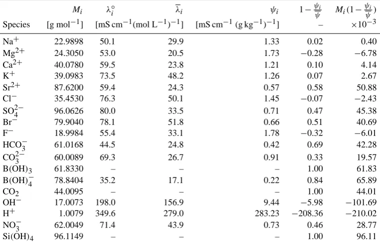
Table 2. Model parameters including molar massesMi, infinite dilution equivalent conductivitiesλ◦i, ionic equivalent conductivitiesλi in
SSW76, conductivities per unit massψi, and coefficients multiplyingδciin the approximateδSsolnR Eq. (30).
Mi λ◦i λi ψi 1−ψψi Mi(1−ψψi)
Species [g mol−1] [mS cm−1(mol L−1)−1] [mS cm−1(g kg−1)−1] – ×10−3
Na+ 22.9898 50.1 29.9 1.33 0.02 0.40
Mg2+ 24.3050 53.0 20.5 1.73 −0.28 −6.78
Ca2+ 40.0780 59.5 23.8 1.21 0.10 4.14
K+ 39.0983 73.5 48.2 1.26 0.07 2.67
Sr2+ 87.6200 59.4 24.3 0.57 0.58 50.88
Cl− 35.4530 76.3 50.1 1.45 −0.07 −2.43
SO24− 96.0626 80.0 33.5 0.71 0.47 45.38
Br− 79.9040 78.1 51.8 0.66 0.51 40.69
F− 18.9984 55.4 33.1 1.78 −0.32 −6.01
HCO−3 61.0168 44.5 24.8 0.42 0.69 42.28
CO23− 60.0089 69.3 26.7 0.91 0.33 19.57
B(OH)3 61.8330 – – – 1.00 61.83
B(OH)−4 78.8404 35.2 17.1 0.22 0.84 65.89
CO2 44.0095 – – – 1.00 44.01
OH− 17.0073 198.0 156.9 9.44 −5.98 −101.69
H+ 1.0079 349.6 279.0 283.23 −208.36 −210.02
NO−3 62.0049 71.4 43.9 0.73 0.46 28.77
Si(OH)4 96.1149 – – – 1.00 96.11
have practical importance in understanding the global circu-lation. A reevaluation of the procedures for determining ther-modynamic properties of seawater, including density, sug-gests that more accurate results can be obtained by returning to a procedure in which absolute salinity is used instead of SP as a state variable (Feistel, 2008; Millero et al., 2008).
In this procedure a best estimateSRfor the absolute salinity
of SSW is made by takingγ=uPS≡35.16504/35≈1.004715.
For non-standard seawaters an offset, which was also called δSA(Millero et al., 2008) but is here denotedδSRdensto
indi-cate that it is found from measurements of density anomalies, is added toSRto calculateSAdensas a best estimate for the
ab-solute salinity (McDougall et al., 2009).
The absolute salinity can be directly estimated by measur-ing the density of water samples and then invertmeasur-ing the equa-tion of state which relates density and salinity. The algorithm forδSRdensprovided by McDougall et al. (2009) is based on a fit of such data against measured Si(OH)4concentrations.
Other algorithms for estimatingδSRdensalso exist (Brewer and Bradshaw, 1975; Millero, 2000). These are also based on purely empirical correlations of density anomalies with con-centrations of specific chemical species, typically nutrients and components of the carbonate system.
However, little work has been done on understanding the full theoretical basis for these corrections. A complete chem-ical theory would include a model for seawater, and a method for determining the variations in conductivity and density that result from compositional variations. Density has been
well-studied (e.g. Millero et al., 1976), but in spite of the practical importance of conductivity in ocean measurements there has been virtually no work done in developing a the-ory of electrical conductivity for natural seawaters. Recently, a model has been developed for calculating the electrical conductivity of natural freshwaters, based on their chemical composition (Pawlowicz, 2008, hereafter Pa08). Although the Pa08 model works well for waters of low salinities (less than a few g kg−1of dissolved solids), accuracy in waters of higher salinities is not sufficient to directly replace the em-pirical relationship specified by PSS-78. However, it will be shown here that the model can be used to quantitatively cal-culate the effects of small compositional variations on the known PSS-78 conductivity/salinity relationship.
The purpose of this paper is then twofold. First, to develop a seawater conductivity model, based on Pa08, capable of quantitatively determining the effects of small variations in the chemical composition of a model seawater on its conduc-tivity, and consequently on SP. Second, to use this model
2 Methods
The general approach is based on modeling perturbations about a known base state for SSW. The base state consists of the known PSS-78 relationship (Eq. 1), and a chemical composition which is a function of the practical salinity.
The first step is then to construct the model composition C∗ for SSW, with an assumed practical salinity SP*, true
conductivityκ∗=f78−1(SP*), and computed reference salinity
(via Eq. 2)S∗=γ SP*, which in this case equals the absolute
salinity. The compositionC∗will be based on a model of the
changes arising from dilutions and evaporations of a refer-ence compositionC0for whichSP=35. Thus our seawater
model will mimic the seawater used to develop PSS-78, and can be used to estimateγ.
The second step is to compute conductivity and abso-lute salinity perturbations,δκandδS∗solnrespectively, arising from compositional changes. There are two kinds of calcu-lation possible. The most straightforward occurs when an initial base stateC∗is known, and a known perturbationδC∗
is added. The Pa08 conductivity model is used to estimate δκ. In this calculation a nonzero offsetδSRsoln can arise be-cause both absolute and conductivity-based reference salini-ties change (to values ofSAsolnandSRrespectively), but
gen-erally by different amounts. Since these situations often in-volve composition changes only in the nonconservative ele-ments of seawater, we call this a constant chlorinity calcula-tion. However, estuarine situations when freshwaters (which may contain Cl−and other so-called conservative elements) are added will also be handled in this way. Results can be simplified into an approximate analytical form, which can then be used to qualitatively understand the effect of pertur-bations.
In contrast, a more formally correct procedure for the cor-rection of ocean measurements is to computeδSRsoln when the composition is perturbed, but only the final conductiv-ityκ (and hence SR) are known. In this constant
conduc-tivity calculation the addition of a known concentration of (say) nitrate, which is ionic and would increase conductivity, would be balanced by a small dilution of the SSW composi-tion corresponding to the measuredSR, in order to keep
con-ductivity constant. The Pa08 model is then used iteratively to calculate the dilution factor, such that the conductivity of final composition composed of diluted SSW plus the compo-sition anomaly matches the measurement. A changeδSRsoln(2) is found by subtracting the initialSRfrom the absolute
salin-ity of the final composition. The compositional perturbations are small in the examples considered here, and the two proce-dures provide nearly identical values for the offset associated with a given composition anomaly.
Unless otherwise stated, all calculations are carried out for a temperature of 25◦C and a sea pressure of 0 dbar. This is appropriate for comparisons with laboratory measurements on water samples. The accuracy of the Pa08 conductivity
model has also been most comprehensively investigated un-der these conditions.
2.1 A composition model for standard seawater (SP=35)
Typical oceanic concentrations of virtually all elements in the periodic table are now known (e.g., Nozaki, 1997), but many elements are present in only trace quantities. The model base state (labelled SSW76, see columns 1–2 of Table 3) is meant to match as closely as possible the composition of SSW de-rived from North Atlantic surface seawater circa 1976 used to determine both PSS-78 and the 1980 equation of state (Millero and Poisson, 1981). It includes all components that can affect salinity down to the level of 1 mg kg−1, although traditional practice in not including the dissolved gases N2
(16 mg kg−1), and O
2(0–8 mg kg−1) is followed. This
com-position is denoted by a vectorC0= {c1c2... cNc}, whereci
is the concentration (mol kg−1solution) of theith ofNc
con-stituents. SSW76 is defined to haveSP=35 (exactly), and
constructed to have a chlorinityClof 19.374 g kg−1 accord-ing to the definition (Millero et al., 2008) derived from titra-tion procedures:
Cl/(g kg−1)≡0.3285234·MAg·([Cl−] + [Br−] + [I−]) (5)
with [·] denoting concentrations and MAg =
107.8682 g mol−1 the molar mass of silver. In addi-tion, the reference salinitySR≡uPSSP(Millero et al., 2008),
will be (exactly) 35.16504 g kg−1.
The recently defined reference composition of standard seawater (from Millero et al., 2008, hereafter M08) was taken as a starting point in specifying SSW76. However, M08 can-not easily be used directly as a model for seawater in this study for several reasons.
First, the fixed ratios of carbonate system components in M08 are not convenient for studying spatial and temporal variations in seawater composition. Although specification of the carbonate system in seawater requires (at minimum) 7 species (Millero, 1995), some of which appear in amounts much less than 1 mg kg−1, their concentrations are not in-dependent. Rather, they are coupled by constants governing the chemical equilibria between them. Only two parameters from the set{TA, pH, f CO2, DIC}are required to fully
spec-ify the carbonate system (with minor corrections arising from borate and SO24−concentrations). From these parameters, the equilibrium constants (denoted by Kw,K0,K1,K2,KB and
parameterized in Dickson et al., 2007) are used to compute the ionic concentrations.
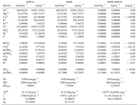
Table 3. The chemical compositions of model SSW76, NPIW, and their differences. For both water types we show concentrations in molar
units and their contribution to mass-based salinities. The upper 9 species are conservative. Both SSW76 and NPIW have a chlorinity of
19 374 mg kg−1, but chlorinity is not exactly the same as the concentration of Cl−(Millero et al., 2008). The next 7 species form the
carbonate system, followed by the two nutrients. We also list other parameters that can be used to specify the equilibria involved in the
carbonate system. SAsoln,κ,SP, andSRare computed according to the formulas discussed in the text. The charge differences in the
right-most column are indicated with two signs. The first represents the net change (increase or decrease), and the second whether these are positive or negative charges.
SSW76 NPIW NPIW-SSW76
Species mmol kg−1 mg kg−1 mmol kg−1 mg kg−1 mmol kg−1 mg kg−1 µeq kg−1
Na+ 468.96335 10781.35913 468.96335 10781.35913 0.00000 0.00000 0.00
Mg2+ 52.81702 1283.71757 52.81702 1283.71757 0.00000 0.00000 0.00
Ca2+ 10.28205 412.08380 10.37705 415.89129 0.09500 3.80748 + +190.00
K+ 10.20769 399.10324 10.20769 399.10324 0.00000 0.00000 0.00
Sr2+ 0.09066 7.94332 0.09066 7.94332 0.00000 0.00000 0.00
Cl− 545.86954 19352.71293 545.86954 19352.71293 0.00000 0.00000 0.00
SO24− 28.23526 2712.35228 28.23526 2712.35228 0.00000 0.00000 0.00
Br− 0.84208 67.28578 0.84208 67.28578 0.00000 0.00000 0.00
F− 0.06832 1.29805 0.06832 1.29805 0.00000 0.00000 0.00
HCO−3 1.90028 115.94926 2.25090 137.34304 0.35062 21.39378 +−350.62
CO23− 0.16285 9.77242 0.08222 4.93414 −0.08063 −4.83828 − −161.25
B(OH)3 0.34579 21.38143 0.38239 23.64422 0.03660 2.26279 0.00
B(OH)−4 0.06923 5.45779 0.03263 2.57262 −0.03660 −2.88517 − −36.60
CO2 0.01687 0.74233 0.04687 2.06284 0.03001 1.32051 0.00
OH− 0.00480 0.08172 0.00205 0.03483 −0.00276 −0.04688 − −2.76
H+ 0.00001 0.00001 0.00002 0.00002 0.00001 0.00001 + +0.01
NO−3 0.00000 0.00000 0.04000 2.48020 0.04000 2.48020 + -40.00
Si(OH)4 0.00000 0.00000 0.17000 16.33953 0.17000 16.33953 0.00
TA 2300.0 µeq kg−1 2450.0 µeq kg−1 150.0 µeq kg−1
DIC 2080.0 µmol kg−1 2380.0 µmol kg−1 300.0 µmol kg−1
pHTOT 7.89892 7.52859 −0.37033
SAsoln 35.17124 g kg−1 35.21108 g kg−1 δS∗soln=0.03983 g kg−1
κ 53064.8 µS cm−1 53073.1 µS cm−1 δκ=8.324 µS cm−1
SP 35.00000 35.00618 δSP=0.00618
SR 35.16504 35.17125
TA≡ [HCO−3] +2[CO23−] + [B(OH)−4] + [OH−]−[H+] (6) A total borate component is specified by adding together the B(OH)−4 and B(OH)3components of M08, and SO24−
con-centrations (required for carbonate system calculations) are also taken from M08.
Second, although the TA of SSW76 and M08 are the same, the total dissolved inorganic carbon (DIC) defined as DIC≡ [CO2] + [HCO−3] + [CO23−] (7)
in the two models is different (as are pH and f CO2). The
reason for this is that attempts to matchδSAsolnobservations,
as well as weak independent evidence, suggest that the DIC content of SSW is somewhat higher than that specified in M08.
M08 specifies ionic composition after setting the fugacity
f CO2to 333 µ-atm at a temperature of 25◦C. This f CO2is
appropriate for an equilibrium with atmospheric levels when the measurements were made to define PSS-78, and at 25◦C
implies a DIC of 1963 µmol kg−1. Typically, after sampling, SSW is filtered and sterilized for≈30 days at temperatures of 28◦C before 1991 (batch numbers up to P115), but only 18– 21◦C since then (P. Ridout, OSIL, personal communication, 2009). Since the solubility of CO2is strongly dependent on
and at 28◦C they would be 1937 µmol kg−1. The change
in DIC due to increasing atmospheric CO2levels is slightly
smaller. At a temperature of 25◦C and a present-day f CO 2
of 380 µ-atm, calculated DIC would be 1992 µmol kg−1. However, there are indications that measured DIC val-ues in ampoules of SSW are often (but not always) some-what higher than these predicted equilibriums at bottling time, and this is generally believed to be caused by the de-composition of residual organic matter after bottling. Un-fortunately, although the TA of standard seawater has been studied (Goyet et al., 1985; Millero et al., 1993), there has been no systematic attempt to analyze the DIC content of standard seawater, and its temporal stability. Brewer and Bradshaw (1975) measured 2238 µmol kg−1 in SSW batch P61. Recent (September 2009) measurements of DIC in am-poules of old SSW from batches P79 (from 1977), P111 (1989), and bottled P140 (2000) found values of 2610, 2200, and 1803 µmol kg−1, respectively. The spread between replicates from different ampoules of the same batch was 10–20 µmol kg−1, larger than measurement uncertainty, but much smaller than the variations between batches.
In fact, as will be shown later, conductivity is not sensitive to variations in DIC, although SsolnA (and henceδSRsoln) are greatly affected. A DIC change of 100 µmol kg−1 is equiv-alent to an absolute salinity variation of≈0.006 g kg−1, but will changeSP by only 0.0007. Since a primary purpose of
ourδSRsolncorrections is (eventually) to calculate densities, it may be more important to choose a model DIC value that will match that of the water used in the measurements defining the 1980 equation of state (Millero and Poisson, 1981), relat-ing salinity and density. This is stated by Millero (2000) to have been 2226 µmol kg−1. However, density fits to Pacific ocean data published in that paper also suggest zero density anomalies occur when DIC=2000 µmol kg−1.
Since ampoules of SSW are sealed, this large range of un-certainty is ultimately related to the effects of organic mate-rial and its neglect in the inorganic seawater chemistry model developed here. This makes it difficult to specify a useful model value for DIC in advance of any calculations, although both density measurements and direct observations suggest concentrations somewhat higher than that of M08. It is probably desirable that our definition (eventually) imply that δSRsoln≈0 for observations from the surface North Atlantic. Thus, after some tuning, DIC is set to 2080 µmol kg−1.
An inappropriate value for the DIC of SSW76 will (even-tually) lead to a near-constant offset in all calculated abso-lute salinity variations. Although this offset is thus poten-tially significant, it will apply to all calculations and hence may have little effect on comparisons between different sea-waters, or on any computation in which additions rather than absolute levels of DIC are specified.
The last difference is that non-conservative nutrient species must be included. Changes in NO−3 and Si(OH)4will
exceed 1 mg kg−1in a seawater withSR≈35 g kg−1and are
related to the salinity variations we seek to model (Brewer and Bradshaw, 1975; Millero, 2000). These nutrients are as-sumed to have a concentration of zero in SSW76.
Following customary practice the mass of Na+is adjusted slightly to maintain charge neutrality, once all other ionic components are specified in SSW76. This may partly ac-count for the contributions of neglected ionic constituents, of which the most important are the conservative elements Li+(0.18 mg kg−1, Soffyn-Egli and Mackenzie, 1984), Rb+ (0.12 mg kg−1), and the nutrient PO−4 (0–0.23 mg kg−1).
The computed absolute salinitys(C0)is 35.171 g kg−1for
SSW76. This differs by 0.006 g kg−1from the defined value
ofSRfor SSW of 35.16504 g kg−1. The mismatch is within
the uncertainty of±0.007 g kg−1suggested by Millero et al.
(2008), although much of that error arises from uncertainty about the amount of SO24−. In contrast, the salinity difference here largely arises from differences in carbonate parameters. However, it should be emphasized that SSW76 is a model of seawater, and not necessarily a better (or worse) description of actual seawater than M08. This is because the assumed precision for some of the constituent concentrations is greater than that of the best observations.
Strictly speaking, the difference between γ=35.171/35 anduPS means that the offsets computed in this paper are
is not exactly those required to get the true absolute salin-ity. Instead they will be in error by a scale factor of γ /uPS≈1.00017. However, the difference is small enough
that it is not of any practical importance and the difference will be ignored.
2.2 A model for standard seawater (SP6=35)
The composition of SSWC∗at practical salinities other than
35 can be specified in different ways. The simplest is to mul-tiply all constituent concentrations by a constant fraction (i.e. C∗(3)=β·C0forSP*=β·35). This is a so-called type III
Ref-erence Seawater (Millero et al., 2008). However, during the specification of PSS-78, SSW was evaporated or diluted with distilled water in order to change its salinity, and again equi-librated with the atmosphere. This makes it more reason-able to specify a type II Reference SeawaterC∗(2), where only
the concentrations of conservative tracers, as well as TA, are multiplied by the constant fractionβforSP*=β·35, but f CO2
is kept constant.
Assuming in advance of our later discussion that the con-ductivity model can predict the effects of perturbations rea-sonably well, and realizing thatC∗(2) andC∗(3)are very
sim-ilar, the differences in conductivity, absolute salinity, and conductivity-derived practical salinity arising from these two approximations can be estimated as:
δκ0=κPa08(C∗(2))−κPa08(C∗(3)) (8)
δSP0=f78(κPa08(C∗(2)))−f78(κPa08(C∗(3))) (10)
whereκPa08is the conductivity estimate computed using the
Pa08 conductivity model and the two absolute salinities in Eq. (9) are calculated using Eq. (2).
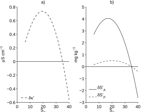
Over the range of 5<SP<40, the conductivity
differ-ences areδκ0<±0.8 µS cm−1(Fig. 1a), which in turn implies δSP0<±0.0005 (Fig. 1b). These uncertainties are negligible. However, the changes in absolute salinityδSA0 are an order of magnitude larger, and can approach 0.004 g kg−1at salin-ities of about 17 (Fig. 1b) although the differences are not important for typical seawater salinities near 35.
2.3 A perturbation model for observed seawater
As a particular parcel of seawater is advected through the ocean, biogeochemical processes alter its composition so it differs from that of SSW. These perturbations are represented by a vectorδC∗, so that the composition becomesC∗+δC∗.
Biogeochemical processes will not alter the unreactive com-ponents of seawater, so these comcom-ponents ofδC∗ are zero.
Changes occur due to variations in non-conservative nutri-ents and componnutri-ents of the carbonate system. However, cal-culations appropriate for estuarine waters may also involve changes in some of the unreactive components as they may also be components of freshwaters.
Note that a slight simplification has been made. Ac-tual additions of a particular species to a volume of water will (slightly) change the concentrations of all other species, when concentrations are measured per unit mass of solution (or per unit volume) as is done here. However, modeling this additional complication is not necessary here as we are not tracking individual parcels.
Nutrient changes that lie above our threshold of 1 mg kg−1 include nitrate (NO−3) and silicate. The latter can appear in the form of SiO2, Si(OH)4, and SiO(OH)−3. Typically in
the pH range of seawater all but a few percent appears as nonconductive Si(OH)4, and it will therefore be assumed that
only a negligible amount appears in the other forms. Changes to the carbonate system can be determined by measurements of TA and DIC (or any two equivalent mea-surements, e.g. pH and TA). With the addition of NO−3, and a change in TA, the number of positive and negative charges in the composition will probably no longer balance. Other processes must therefore be present in the real ocean to bal-ance this excess (or rather, the change in TA arises to com-pensate for the effects of these other processes). The dissolu-tion of CaCO3is likely the predominant mechanism at work
(Sarmiento and Gruber, 2006). The negative charges and car-bon from CO23−are already accounted for in the increase in TA and DIC respectively. An increase in Ca2+is also known to occur in deep waters (de Villiers, 1998), and we assume that this will balance the change in total charge. That is, we
0 10 20 30 40
−3 −2 −1 0 1 2 3 4 5
S
P
mg kg
−1
b)
δS’
A
δS’
P
0 10 20 30 40
−0.6 −0.4 −0.2 0 0.2 0.4 0.6 0.8
S
P
μ
S cm
−1
a)
δκ’
Fig. 1. Comparison between constant f CO2and constant fraction models for dilution of seawater. (a) Difference in conductivities.
(b) Differences in practical and absolute salinity.
assume a relationship between the increase in TA and the in-crease in concentrations of Ca2+from dissolution and NO−3 from remineralization:
1TA=21[Ca2+]−1[NO−3] (11)
where1denotes changes. Thus our perturbations must in-clude measured concentrations of NO−3, Si(OH)4, TA, and
DIC, as well as an inferred change in Ca2+using Eq. (11). Carbonate parameters are then recomputed using the equilib-rium constant formulas described by Dickson et al. (2007).
Of course, other processes also occur in the ocean. For ex-ample, TA also varies with changes in phosphate and organic substances, although these contributions will fall below our threshold of importance. A more important process might be sulfate reduction on continental shelves (Chen, 2002), which may be responsible for a large part of TA increases in some areas. In order to model this situation Eq. (11) would be modified to:
1TA=21[Ca2+]−21[SO42−]−1[NO−3] (12) but now an additional relationship (specifying, e.g., the im-portance of CaCO3dissolution relative to SO24−reduction) is
needed to complete the model. Speculation on this relation-ship is beyond the scope of this paper.
2.4 A model for seawater conductivity
The Pa08 model estimateκPa08of the true electrical
conduc-tivityκ of a dilute multi-component aqueous ionic solution like seawater is computed using an equation which can be written in a simplified form as (Pawlowicz, 2008)
κPa08(C)=
Nc
X
i=1
λic∗izi (13)
The in-situ ionic equivalent conductivitiesλi=λ◦ifiαiare the
product of infinite dilution equivalent conductivitiesλ◦i for the different ions (set to zero for nonionic species), and two reduction factors: fi(I∗)≤1, accounting for relaxation and
electrophoresis effects, andαi(I∗,C)≤1, accounting for ion
association effects at finite ionic strengthI∗. The stoichio-metric ionic strengthI∗is
I∗=1 2
Nc
X
i=1
z2ic∗i (14)
The valence of charge on theith ion isziand its
stoichiomet-ric concentrationc∗i (mol L−1). This is related toci through
a density equation (Millero and Poisson, 1981):
ci∗=ρ(SP)ci (15)
where we incur an error of at most 1×10⁻⁵by ignoring the fact that the true density will change slightly with composi-tion perturbacomposi-tionsδC∗. AsI∗→0 we havefi→1 andαi→1.
The relaxation/electrophoresis reduction parameterfi for
speciesidepends on the concentrations of other speciesj6=i only through their contribution toI∗. However, the ion as-sociation parameterαi depends critically on the
concentra-tions and identities of all other ions (i.e. on the total set of ci∗,i=1,...,Nc), as it is a weighted sum of interactions with
all other anions (cations) for a cation (anion). In order to ac-count for this the internal model structure is somewhat more complicated than Eq. (13) suggests. Both the infinite dilu-tion equivalent conductivities, and the in-situ ionic equiva-lent conductivities determined by Pa08 for SSW76, are listed in Table 2.
The conductivity model used is identical to that described in Pa08, with the addition of parameters for B(OH)−4, de-rived from observations of Corti et al. (1980). All numerical parameters are based purely on basic chemical measurements in binary solutions, without reference to any measurements made in seawater (or any other natural water).
The accuracy of the computed conductivityκPa08depends
on the accuracy of the measured ionic concentrationsci∗, as well as on biases in the calculation of the reduction fac-tors fi and αi. At salinities <4 g kg−1 the relative
accu-racy ε=(κPa08−κ)/κ of the model is typically limited to
±0.03 by the accuracy of the chemical analyses used to de-termine composition (unpublished results). Once this error
is reduced, by, e.g., statistical averaging, the true error is less than 0.007 over a range of chemical compositions. For sea-water with salinities of 0.1–1 g kg−1we find an overestimate
of only 0.002. However, at the higher salinities of concern here model biases dominate the error, withεsmoothly vary-ing from about−0.01 at a salinity of 4 (κ∼8 mS cm−1) to about−0.10 at a salinity of 35 orκ∼50 mS cm−1(Fig. 2b). 2.5 Conductivity perturbations for non-standard
seawaters
A salinity underestimate of order 3 g kg−1resulting from us-ingκPa08in Eq. (1) directly will not allow us to directly
in-vestigate the small compositional variations in typical sea-water that we have discussed above, which are several or-ders of magnitude smaller. However, not only is|ε|1, but it is relatively insensitive to changes in chemical composi-tion. A comparison of measured and predicted conductivi-ties for a variety of saline ocean and lake waters in the range of 20–50 mS cm−1 (Fig. 2b) shows that the resulting error is virtually identical for different compositions at the same conductivity. This is very different from results found when considering baseline predictions formed by takingfi=αi=1,
or equivalently using infinite dilution equivalent conductivi-ties for the different components, ignoring all interionic in-teractions (Fig. 2a). Not only are these baseline predictions greatly in excess of true conductivities (so thatε=O(1)), but the excess is highly sensitive to the composition. The base-lineεfor Mahoney Lake is almost double that for seawater at the same conductivity. The model is therefore accounting for relative chemical composition correctly, but with an overall bias that depends (weakly) on the salinity.
Thus for model predictions during which only small changesδC∗in composition are made, we can take theκPa08
errorε≈constant.εis estimated from
κ(C∗)=κPa08(C∗)·(1+ε)−1 (16)
knowing that κ(C∗)=f78−1(SP*) for SSW76. Since we
as-sume
κ(C∗+δC∗)≈κPa08(C∗+δC∗)·(1+ε)−1 (17)
the change in conductivityδκ related to small compositional changes is:
δκ ≡κ(C∗+δC∗)−κ(C∗)
≈(κPa08(C∗+δC∗)−κPa08(C∗))·(1+ε)−1
=δκPa08·(1+ε)−1 (18)
Thus it appears that we can use Pa08 to usefully predict con-ductivity perturbations.
0 20 40 60 80 100 0 20 40 60 80 100 120 140 160 180 200
Measured conductivity (mS cm−1)
b) Pa08
L. Issyk−Kul Mahoney L. Mono L.
Seawater (SP=1−40)
0 20 40 60 80 100
0 20 40 60 80 100 120 140 160 180 200 a) Baseline
Predicted Conductivity (mS cm
−1
)
Fig. 2. Predicted versus measuredκat 25◦C for saline lakes Ma-honey (Hall and Northcote, 1986), Mono (Jellison et al., 1999), and Issyk-Kul (Vollmer et al., 2002), as well as for seawater. (a) Baseline predictions without ionic interactions. (b) Pa08 predic-tions that include ionic interacpredic-tions. Vertical bars show uncertainty based on the computed charge imbalance in the published chemical composition used for predictions. Lake Issyk-Kul is a warm deep
lake with roughly equal amounts of NaCl and MgSO4,
meromic-tic Mahoney Lake is dominated by NaSO4, Mono Lake contains a
Na−CO3−Cl−SO4brine and seawater is primarily composed of
NaCl.
First, direct estimates of the ionic equivalent conductivi-tiesλi=λ◦ifi in seawater have been made using a
radioac-tive tracer technique (Poisson et al., 1979). These parame-ters can also be extracted from the Pa08 model. When using the baseline (i.e. ignoring all modeled ionic interactions) the parameters are overpredicted with relative errors of 0.34 to 1.5 (Fig. 3a). However, when using the full Pa08 model, pre-dictions are much closer to measured values, and the scatter is also greatly diminished. The mean relative error is−0.09, almost identical to that found for conductivity itself.
Note that although the equivalent conductivities are gen-erally underpredicted, the results for SO24− show a slight overprediction. This ion associates strongly with most other cations. This makes it more difficult to model the equivalent conductivity of the ion, as pairing effects must be subtracted from measurements, but also tends to reduce the error when making predictions in actual solutions, as pairing effects are added back in.
More relevant results can be obtained by comparison with so-called partial equivalent conductivities31i, defined by
31i=
∂κ ∂Ei
P ,T ,E
j6=i,...
(19) These have been evaluated from laboratory measurements in which small changes in equivalent concentrationsEi of the
ith of theNs salts (i.e. binary compounds) in seawater are
0 50 100
0 20 40 60 80 100 120 140 160
← Na+
←← Ca Mg2+2+
← K+
Cl−
→ SO
42−→ HCO
3−→
← Br−
Observed ionic equivalent conductivities
(S cm2 eq−1)
Predicted conductivities (S cm
2 eq
−1 ) a) Pa08 Baseline 10% Error
0 50 100
Observed partial equivalent conductivities
(S cm2 eq−1) ← NaCl NaBr → NaF → NaHCO 3→
← KCl KBr
→
KHCO
3→
← MgCl
2
← CaCl
2
← Na
2SO
4
← K
2SO
4
← MgSO
4
b)
← NaCl NaBr → NaF → NaHCO 3→
← KCl KBr
→
KHCO
3→
← MgCl
2
← CaCl
2
← Na
2SO
4
← K
2SO
4
← MgSO
4
b)
0 50 100
Observed partial equivalent conductivities
(S cm2 eq−1) ← NaCl
← KCl
← Na
2SO
4
← K
2SO 4 KHCO 3→ NaHCO 3→
← MgSO
4
← MgCl
2
← CaCl
2
c)
Fig. 3. Comparison between different Pa08 model-derived and
mea-sured parameters related to conductivity, for seawater. (a) Ionic
equivalent conductivities in seawater ofSP=38.38 at 25◦C.
Orig-inal data from Poisson et al. (1979, Table 3). (b) Partial
equiv-alent conductivities for various salts in seawater ofSP=35.13 at
25◦C. Original data from Poisson et al. (1979, Table 4). (c) Partial
equivalent conductivities for various salts in seawater ofSP=35.04
at 23◦C. Original data from Conners and Weyl (1968, Table 4).
Dashed line shows a relative error of−0.10. Baseline predictions
are made by ignoring all ionic interactions (i.e. using only infi-nite dilution equivalent conductivities). Pa08 results include relax-ation/electrophoresis and ion pairing effects, with the former ac-counting for most of the reductions from baseline.
made by additions to a reference seawater (Park, 1964; Con-ners and Park, 1967; ConCon-ners and Weyl, 1968; ConCon-ners and Kester, 1974; Poisson et al., 1979). The data are corrected to show the derivatives when all other other conditions, and concentrations of all other ions, are held fixed. Note that the 31i are not equal to the sum of the corresponding equivalent
conductivities for the anion and cation in Eq. (13) when eval-uated at the ionic strength of seawater. Differences arise due to changes in the ionic strength, and in the effects of pairing (i.e., whenα<1) between the components of the added salt and all other constituents in seawater. However, the31i can
2.6 Salinities of non-standard seawaters
The change in practical salinity resulting from a perturbation δC∗added to an initial compositionC∗is given by
δSP≡SP(C∗+δC∗)−SP(C∗) (20)
=f78(κ(C∗+δC∗))−f78(κ(C∗)) (21)
≈f78(κ(C∗)+δκPa08·(1+ε)−1)−f78(κ(C∗)) (22)
whereε andδκPa08 are as defined in the previous section.
At low salinities whereκPa08has minimal bias the simpler
approximation
δSP≈δSP∗≡f78(κPa08(C∗+δC∗))−f78(κPa08(C∗)) (23)
provides an alternative method of estimating practical salin-ity changes which does not rely on assumptions about the magnitude of perturbations. In fact the function f78(κ)is
smooth enough that the approximation holds to a degree of accuracyεover all salinities (cf. Eq. 10), although we con-tinue to use the computationally more intensive Eq. (22) un-less otherwise specified. In addition to these changes in prac-tical salinity, perturbationsδC∗also lead to changes in abso-lute salinity according to:
δS∗soln≡s(C∗+δC∗)−s(C∗)=s(δC∗) (24)
(by the linearity of Eq. 2).
If we consider a parcel of water with fixed chlorinity, ad-ditionsδC∗ will therefore affect both the measuredSP and
calculated absolute salinity. These changes will generally be different, giving rise to a salinity correction which can be es-timated as:
δSRsoln(1)≡SAsoln(C∗+δC∗)−γ SP(C∗+δC∗) (25)
=δS∗soln−γ δSP (26)
≈δS∗soln−δSP (27)
This implies thatδSRsolnis approximately the change in ab-solute salinity, minus whatever compensating effects arise from conductivity. If a nonionic substance is added,δSsoln∗ will dominate the correction. On the other hand, adding very light but extremely conductive ions could lead to negative corrections arising mostly from changes inSP.
However, when converting ocean measurements to abso-lute salinity we are concerned with the corrections that arise whenSPis held constant, rather than those for fixed
chlorin-ity. For non-standard seawater with a measuredSPwe begin
with a compositionCRappropriate for SSW of the sameSP.
However, the actual composition isβCR+δC∗. That is, the
addition of other solids that dissociate into ions which in-crease conductivity must be matched by a slight dilution of our initial standard seawater composition in order to keep conductivity constant. The dilution factorβ for the SSW composition can be found by solving
κ(βCR+δC∗)=κ(CR) (28)
which can be done iteratively, usingκPa08in place ofκ on
both sides of the equation. Then from Eqs. (4) and (28) the true correction is:
δSRsoln(2)=s(βCR+δC∗)−s(CR)
=δSsoln∗ −(1−β)s(CR) (29)
Typicallyβ is very close to 1 andδSRsoln(1) is within a few percent of δSRsoln(2) for the small perturbations of concern here. Although the latter is technically more correct for deal-ing with ocean data, the advantage of the former is that we can separately estimate effects of changing mass and chang-ing number of electrical charges. We use the notationδSRsoln when the distinction is unimportant.
3 Results
To illustrate the effects of compositional changes δC∗ first
consider an extreme, but realistic, scenario. Investigations of the relationship between salinity and density suggest that largest salinity anomalies (of order 0.03 g kg−1) occur in the
intermediate North Pacific (McDougall et al., 2009). This water represents the endpoint of the subsurface branch of the thermohaline circulation and thus provides an appropriate ex-treme. For comparative purposes model “North Pacific Inter-mediate Water” (NPIW) is normalized to have the same chlo-rinity as SSW76, although actual chlorinities in the North Pacific are about 0.3 g kg−1lower. Based on typical observa-tions, take this water to contain Si(OH)4=170 µmol kg−1and
NO−3=40 µmol kg−1, with TA and DIC larger than in SSW76 by values of 150 µeq kg−1 and 300 µmol kg−1 respectively. Columns 4–5 of Table 3 then contain the model composi-tionC0+δC∗representing NPIW, with the perturbationδC∗
in columns 6–8.
Carbonate equilibria are recalculated from the new TA and DIC. pH on the Total scale drops to about 7.5 (again, all calculations are at 25◦C). The increases we specify actually
cause concentrations of CO23−and B(OH)−4 to decrease sig-nificantly. In addition, charge balance considerations require that the concentration of Ca2+increase by 0.095 mmol kg−1 or a little less than 1% over its value in SSW76. Measured increases in Ca2+ at depth in the North Pacific are of this order (de Villiers, 1998).
Applying the model directly (i.e. under conditions of fixed chlorinity)δSP≈0.0062 andδS∗soln≈0.0398 g kg−1, and
hence from Eq. (27)δSRsoln(1)≈0.034 g kg−1. The cruder ap-proximationδSP∗≈0.0054 underestimatesδSRsolnwith a rela-tive error of only−0.12. A similar calculation, i.e., one with the same changes in TA, DIC, NO−3, and Si(OH)4, under
conditions of fixed conductivity, results in a dilution factor of β=0.9998105, and from Eq. (29)δSRsoln(2)≈0.033 g kg−1.
salinity. The Si(OH)4 component alone contributes about
0.016 g kg−1toδSsoln
R , or almost half of the correction. Much
of the remainder arises primarily due to increases in HCO−3, but there are both increases and decreases in other con-stituents. In fact, the changes in absolute salinity due to the increase in carbonates outweigh those due to the increase in Si(OH)4, but some of this carbonate ion increase is
compen-sated by an increase inSP.
In order to better understand these values we investi-gate the conductivity. Model calculated ionic equivalent conductivities λi within our seawater are all significantly
smaller than the infinite dilution equivalent conductivitiesλ◦i (columns 3 and 4 of Table 2), but with the exception of H+ and OH− are all of order 30 mS cm−1 (mol L−1)−1. Very roughly then, conductivity changes will be proportional to changes in the number of charge pairs present. There are large changes in the concentrations of individual negative ions (last column of Table 3), but overall the increases and decreases in negative ions tend to balance out, matching (in total) the smaller increase in positive charges from Ca2+
pro-duced by CaCO3dissolution. Thus changes in absolute
salin-ity are most strongly influenced by changes in Si(OH)4and
DIC, but changes in practical salinity occur mostly due to CaCO3dissolution.
Further insight can be obtained by deriving an approxi-mate relationship between δSRsoln and δC∗. Seawater
con-ductivity per unit mass of salt at 25◦C in the model is ψ=κPa08/SAsoln≈1.35 mS cm
−1 (g kg−1)−1. Combining
Eqs. (2), (4), and (13) and definingψi=λiziρ/Mias the
con-ductivity per unit mass of theith component:
δSRsoln≈X
i
Mi(1−
ψi
ψ)δci (30)
with numerical values appropriate for SP=35 given in
Ta-ble 2. This expression illustrates the way in which the con-tribution of individual ions toδSRsoln depends on the degree by which conductivity per unit massψi differs from the
av-erageψ. The relationship is only approximate because theψ are not in fact constant, but will also vary withδC∗. In
us-ing this formula it is also important to recall that only charge balanced perturbations are meaningful, so that any scenario must involve changes in at least one cation and anion.
Examination of the mass effect coefficients(1−ψi/ψ )for
different ions (listed in column 6 of Table 2) shows concen-tration perturbations in some ions (e.g., Na+, Ca2+, Mg2+, K+, Cl−, F−) result in little change to δSRsoln. These ions contribute to conductivity in an “average” way, withψi≈ψ.
Contrariwise, concentration changes in other ions do not af-fect conductivity in an average way and hence must be ac-counted for with a non-zeroδSRsoln. Some of these (e.g., Sr2+, Br−) vary with the other conservative ions and hence will not appear in realistic perturbations that arise from biogeo-chemical processes. Nonconductive species contribute ex-actly their added mass. Several ions (H+, OH−) have an
extremely large effect on conductivity, relative to their mass. However, the actual in-situ mass changes in these ions are so small that the overall effect on conductivity is minimal.
Sea salt is composed primarily of Na+and Cl−ions (Ta-ble 3). These contribute to conductivity in an average way, and so if there are small perturbations in their mass practi-cal salinity changes will approximately account for the ab-solute salinity change. However, when using the full model, and ignoring nonconductive Si(OH)4, the change in absolute
salinityδS∗solnis≈0.024, about 4 times larger thanδSP. The
salinity perturbation for modeling NPIW is composed largely of HCO−3, for whichψi is significantly different thanψ.
Us-ing Eq. (30) we expect that an HCO−3 perturbation will give rise to a conductivity change that (when converted to salin-ity using the average factorψ) will only account for≈0.3 of the actual salinity change. The dominance of HCO−3 changes inδC∗, and their relatively unconductive nature, explains the
insensitivity of predicted conductivity to variations in our as-sumptions about how seawater dilution should be modeled (cf. Sect. 2.2).
The choice between Eqs. (11) and (12) to balance TA changes will also have some consequences. An addition of Ca2+ will result in a compensating increase in conduc-tivity, not affectingδSRsoln, but an equal decrease of SO24− (which has an equivalent effect on TA) will not result in a fully compensating decrease in conductivity and hence will result in a smallerδSRsoln. For a concentration change of or-der 100 µmol kg−1 (i.e. for NPIW) the difference in δSRsoln computed using the different scenarios is 0.005 g kg−1 us-ing Eq. (30) or 0.008 g kg−1 using the full model. Since we do not have a good knowledge of the actualδci for all
constituents of seawater, we must rely on assumptions about biogeochemical processes to parameterize them. However, our prediction accuracy is then limited by the extent of our knowledge about these processes.
By considering only those ions both important in typical biogeochemical perturbations (i.e. large values in column 7 of Table 3) and with strong effect onδSsolnR (i.e., with large values in the last column of Table 2), Eq. (30) can be further simplified. Only HCO3−, CO23−, CO2, B(OH)3, B(OH)−4,
NO−3 and Si(OH)4 will have significant effects on δSRsoln.
Since all of the carbonate parameters are related, and rela-tionships such as Eq. (11) mean that the NO−3 term is not re-ally independent either, a more sophisticated understanding of the carbonate system may allow a formula for δSRsoln to be written more simply in terms of more general parameters such as TA and DIC.
25 30 35 40 4
5 6 7 8 9
S
P
TA coeff
25 30 35 40 46.6
46.8 47 47.2 47.4 47.6 47.8 48
S
P
DIC coeff
25 30 35 40 34
34.5 35 35.5 36 36.5 37 37.5
S
P
NO
3
− coeff
Fig. 4. Coefficients of the best fit equationδSRsoln=aTA+bDIC+
c[NO−3]to model predictions, as a function of salinity. (a)
Coeffi-cienta. Dashed line shows a best fit curve as a functionT A·SP/35
rather than TA. (b) Coefficientb. (c) Coefficientc.
be fitted to “measurements” calculated by the perturbation model. This is a simpler way to derive more straightforward formulas.
First consider perturbations when SP=35. The model
is used to calculate δSRsoln(2) over a grid of δC∗ points
within a range of 0≤1TA≤0.3 mmol kg−1, 0≤1DIC≤ 0.3 mmol kg−1, and 0≤1NO−3 ≤0.040 mmol kg−1, with Ca2+ again varying according to Eq. (11). Inspection of the results shows thatδSRsoln(2)varies quasi-linearly with the components of the perturbation, and by least-squares fitting the equation
δSRsoln/(mgkg−1)=(47.111DIC+7.171TA +36.571[NO−3]
/(mmolkg−1) (31)
agrees very well with the full calculations, with a misfit standard error of±0.07 mg kg−1 and a maximum misfit of 0.3 mg kg−1.
The DIC coefficient is similar to the theoretical coeffi-cient for HCO−3 (column 7 Table 2), and both the theoreti-cal and fitted NO−3 coefficients are roughly comparable. The ≈20% difference results from both the biogeochemical rela-tionships, as well as variations in the interionic interactions involved in conductivity.
Repeating the above procedure for 25≤SP≤40, we find
that the coefficients in the fit for δSRsoln vary with salinity (Fig. 4). The coefficients for 1DIC and NO−3 vary only weakly (with a change of<10% over the salinity range cho-sen) and in practical terms the variation can be ignored. However, the coefficient for 1TA varies strongly (>50% change over the salinity range chosen), and almost linearly withSP. This suggests that Eq. (31) should be modified for
situations whenSP6=35 by replacing1TA with1TA·SP/35.
Note that the1signifies the change from SSW values at the specified salinity, e.g. the difference between observed TA and 2.300·SP/35 mmol kg−1. We also add in the total mass
of Si(OH)4to produce this final prediction formula:
δSRsoln/(mgkg−1)=(47.111DIC+7.17(SP/35)1TA
+36.571[NO−3] +96.111[Si(OH)4]/(mmolkg−1) (32)
2250 2300 2350 2400 2450 2500 101
102
103
104
μeq kg−1
a) TA
depth (m)
2000 2200 2400 2600
b) DIC
μmol kg−1
7.2 7.4 7.6 7.8 8 101
102
103
104
c) pH
P17 stn 34 A24 stn 119 AO94 stn 29 S04 stn 29
0 10 20 30 40 50 101
102
103
104
e) NO3−
μmol kg−1
0 20 40 60 80 100
d) ΔCa2+
μmol kg−1
0 50 100 150 200
f) Si(OH)
4
μmol kg−1
Fig. 5. Composition perturbations for example stations: North
Pa-cific (WOCE line P17, station 34, 37.5◦N, 135.0◦W, 10 August
2001), North Atlantic (WOCE line A24, station 119, 52.73◦N,
34.71◦W, 22 June 1997) Arctic (AO94 station 29, 87.16◦N,
160.71◦E, 17 August 1994) and Southern Ocean (WOCE line S04,
station 29, 62.02◦S, 134.18◦E, 9 January 1995). (a) TA for all
pro-files. (b) DIC. (c) pH on the Total scale. (d) Computed change 1Ca2+(e) NO−3. (f) Si(OH)4. Vertical dashed lines show values in SSW76.
Note that there may be no easy way to empirically ver-ify the different coefficients with ocean measurements. An empirical fit to data has resulted in the following relationship δSRdens/(mgkg−1)= 50.13(1TA−0.032)+63.101[NO−3]
+96.301[Si(OH)4])/(mmolkg−1) (33)
(Millero, 2000, Eq. (3), rewritten to match the base value for 1TA used here and using a conversion factor of 756 between density and salinity changes as in that paper) which has a similar coefficient for Si(OH)4, but otherwise is numerically
0 0.01 0.02 0.03 0.04 101
102
103
a) N Pacific (P17 stn 34)
depth (m)
0 0.01 0.02 0.03 0.04 101
102
103
b) N Atlantic (A24 stn 119)
depth (m)
δSRsoln(Si)
δS * soln
δS P
δS R soln
0 0.01 0.02 0.03 0.04 101
102
103
g kg−1
c) Arctic (AO94 stn 29)
depth (m)
0 0.01 0.02 0.03 0.04 101
102
103
g kg−1
d) Southern Ocean (S04 stn 29)
depth (m)
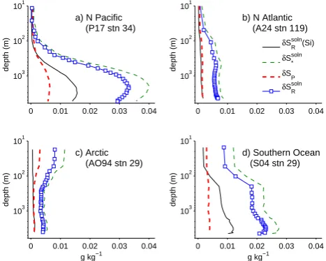
Fig. 6. Predicted corrections for measured water column
pro-files. Shown are the total fixed-conductivity correctionδSRsoln(2),
as well as the components of the fixed-chlorinity correction δSRsoln(1)=δS∗soln−δSP(withδSsoln(2)R ≈δSRsoln(1)), and the
compo-nent of the correction due to silicate alone,δSsolnR (Si). (a) N.
Pa-cific profile. (b) N. Atlantic profile. (c) Arctic profile. (d) Southern Ocean profile.
The full calculation procedure can easily be applied to actual ocean profiles, as long as they include observations of SP, TA, DIC, Si(OH)4 and NO−3. These parameters
are now considered to be standard for deep-ocean hydro-graphic observations so no modification is needed in rou-tine procedures. The latter 4 are enough to specify the non-conservative elements, with changes in Ca2+ inferred from Eq. (11) to maintain charge neutrality.
As an example, consider several recent high-quality hy-drographic profiles from the North Atlantic, Arctic, and North Pacific, and Southern Ocean (Figs. 5–7). Previous δSRdens estimates have been made in all regions except the Arctic.
Surface nutrients are low in all profiles except in the South-ern Ocean, and surface pH relatively high, although lower than in SSW (Fig. 5). The Arctic profile has a high surface TA, which implies higher Ca2+, and DIC, due to cold tem-peratures. Nutrients, TA, and DIC at depth are much higher in the North Pacific than in the other profiles. However, deep pH is much lower. Deep nutrient levels are typically higher than surface nutrients in all cases. Inferred1Ca2+is high in
the Arctic and Southern Ocean, and high in the deep North Pacific.
The computed salinity correctionδSRsoln(2)is close to zero in the surface waters of the N. Pacific (Fig. 6a) and N. At-lantic (Fig. 6b), but is almost 0.008 in the surface waters of the Arctic (Fig. 6c). On the other hand, the correction is low-est at depth in the Arctic (only 0.003), but is as high as 0.033 in the deep North Pacific. The surface correction is highest
0 0.01 0.02 0.03 0.04 101
102
103
a) N Pacific (P17 stn 34)
depth (m)
0 0.01 0.02 0.03 0.04 101
102
103
b) N Atlantic (A24 stn 119)
depth (m)
McDougall et al. (2009) Millero et al. (2008)
δ S
R soln
δ S
R soln(SiO
2)
0 0.01 0.02 0.03 0.04 101
102
103
c) Arctic (AO94 stn 29)
depth (m)
g kg−1
0 0.01 0.02 0.03 0.04 101
102
103
d) Southern Ocean (S04 stn 29)
depth (m)
g kg−1
Fig. 7. Comparison betweenδSRsoln(2)computed with the full con-ductivity model in this paper with the results of empirical formulas
forδSRdensprovided by Millero et al. (2008) and McDougall et al.
(2009). The latter provides corrections as a function of ocean basin,
latitude, and measured Si(OH)4. Also shown are calculations using
a reduced mass for added Si. (a) North Pacific. (b) North Atlantic.
(c) Arctic. (d) Southern Ocean.
in the Southern Ocean. The correction itself is dominated by theδS∗solnin all cases withδSRsoln(2)≈0.8δS∗soln. The increase in ionic content does result in a small change in conductivity which partially compensates for the compositional change, but as beforeδSPδS∗soln.
Comparison of calculatedδSRsoln(2) withδSRdens produced by Eq. (33) and McDougall et al. (2009) for these stations are relatively good (Fig. 7). The general shape of depth profiles and overall magnitudes are similar, although our estimates appear to be systematically slightly larger. Correction factors in the deep Pacific and shallow Arctic are large, but are small in both Pacific and Atlantic surface waters, and deep Arctic waters. Our corrections are about 0.005 larger in the deep Pacific and not very different whenδSsoln(2)R ≈0. Widest dis-agreement between the three estimates occurs in the South-ern Ocean. For all profiles, the modelδSRsoln(2)is the largest of the 3 estimates, and the predictions of McDougall et al. (2009) the smallest.
As a final comparison, the model is used to replicate the measurements in a controlled situation where the chemistry is more precisely known. Millero (1984) measured δSRdens (Fig. 8) for various mixtures composed of a known fraction aof SSW and an artificial river water of known composition CRW(Table 4):
Cmixture=aC0+(1−a)CRW (34)
with 0≤a≤1. Here we take the dilutionC∗=aC0as a base
0 5 10 15 20 25 30 35 0
0.02 0.04 0.06 0.08 0.1 0.12
Salinity (S
R) (g kg
−1)
g kg
−1
or PSU
δS
R soln(1) = δS
* soln−δS
P
δS*soln
δSP
δ SP*
Pa08 δSRsoln(1)
Pa08 δS*soln
Pa08 δSP
Millero (1984) δS
R dens
Fig. 8. Comparison betweenδSRsoln(1)computed with the full
per-turbation model in this paper with the measurements ofδSRdensby
Millero (1984) in mixtures of SSW and artificial river water. Also
shown are direct estimatesδS∗P using the Pa08 model, as well as
limiting case estimates for pure river water using Pa08.
perturbation in a fixed-chlorinity calculation. The name is somewhat misleading here because the river water also con-tains Cl−but this does not affect the mathematical details of
the calculation. Calculations must be modified slightly when SP<5, since the usual seawater parameterizations of the
car-bonate equilibria are no longer valid in this low-salinity range. They do not extrapolate correctly to pure-water lim-its. Instead we use low-salinity parameterizations more suit-able for river and lake waters (Millero, 1995). The change ofδSRsolnacross the transition between the two regimes is not smooth, but the size of the step is small enough that it cannot be seen in Fig. 8.
The δSRsoln(1) arising from perturbation computations al-most exactly lies within the scatter of the observations (Fig. 8). As salinity drops and the riverine addition be-comes a larger fraction of the composition,δSRsolnincreases. One unexpected result is thatδSRsoln(1)increases roughly lin-early with decreases in salinity only at high salinities. When SRdrops below about 10 g kg−1,δSP curves upwards quite
sharply, so that theδSsoln(1)R curve flattens and even decreases at very low salinities. The observations do not appear to show this, although their scatter is large enough that this behavior cannot be ruled out. However, at low salinities where the Pa08 model is known to be accurate (unpublished results), it can be applied directly toCmixtureand the alternative estimate
δSP∗used in place of the perturbation calculation forδSP.
Re-sults agree almost exactly with the perturbation model, show-ing the same curvature. Agreement is good at low salinities because the bias in Pa08 is small, and is good at high salini-ties because the river water perturbation is very small.
Table 4. CompositionCRWof artificial river water used by Millero
(1984). Numbers have been adjusted to correct for typographical errors in Millero et al. (1976) and to agree best with stated values of both molar and mass concentrations in that paper, after rounding. TA is set by charge balance, with DIC carbonate ion concentrations computed from TA and pH using the low-salinity carbonate system
parameterizations of Millero (1995) whenSP<5.
Species Concentration
(mmol kg−1)
Ca2+ 0.3745
Mg2+ 0.1685
Na+ 0.2740
K+ 0.0590
SO24− 0.1165
Cl− 0.2200
NO−3 0.0160
HCO−3 0.9434
CO23− 0.0031
CO2 0.0440
OH− 0.0004
pH 7.60
TA 0.9500 meq kg−1
DIC 0.9905
SAsoln 0.1074 g kg−1
Finally, fora=0 Pa08 directly predicts a conductivity of 142 µS cm−1, which can then be used with PSS-78 to com-puteSP=0.0686 and henceδSRsoln=0.0388 g kg
−1
indepen-dently of the seawater perturbation model. The perturbation model does approach these values in the limit asa→0. Note however that this limit is not a good indicator of the zero-salinity intercept of a best-fit line through the observations, especially those from salinities>5 g kg−1, typical of most estuarine waters, because of the curvature in δSP. Such a
best fit line would intercept the left axis at rather higher val-ues. Overall, however, although the particular chemistry of the oceanic perturbations may result in different errors than those associated with riverine dilutions, there do not appear to be any general biases present.
4 Discussion and conclusions
The combination of a chemical model of seawater and a con-ductivity model allows the effects of compositional pertur-bations on conductivity-based methods of salinity determi-nation to be estimated. An immediate result is that conduc-tivity itself is relatively insensitive to biogeochemical pertur-bations to the chemical composition of seawater. In fixed chlorinity calculations,δSPincreases by less than 0.007 over
(i.e. the scaledSP) lie somewhere between a chlorinity-based
measure and the true absolute salinity, although much closer to the former. This also accounts for the stability of con-ductivity in SSW (Bacon et al., 2007), in spite of the known variations in DIC that occur within samples.
A second result is that the observedδSRsolnare almost en-tirely explained by changes in nutrients and the carbonate system. Although this fact is already known empirically and is the basis for existing estimates ofδSRdens (e.g., Mc-Dougall et al., 2009; Millero, 2000) the model calculations provide a more theoretical confirmation. In addition, the model shows that variations in Ca2+and/or SO−4 are as im-portant as changes in NO−3, although they are linked via bio-geochemical relationships.
Another result is that the effects of perturbations at typical oceanic salinities are approximately linear functions of salin-ity, but that this linear behavior does not extrapolate well to behavior at low salinities (SP<5). At low salinities
carbon-ate composition andδSPbecome much more nonlinear
func-tions of salinity. Thus generalizafunc-tions based on infinite di-lution quantities, or river endpoints, are qualitatively useful but may in practice be less relevant to oceanic situations than might be otherwise be expected. Conversely, extrapolations of linear fits to measurements in estuarine waters will not necessarily agree with observations of river end-members.
However, although the general agreement between calcu-latedδSRsolnand density-based estimates likeδSdensR is good, differences remain. The differences are not very much larger than the typical uncertainty arising from density measure-ments, but are systematic. There are several possible expla-nations for these differences.
First, the Pa08 conductivity model may be inadequate to correctly calculate perturbations in this application. The scatter in comparisons between predictions and observations in Fig. 3 suggests that the model bias may still depend to some extent on chemical composition. It is difficult to fully address this issue without more data for comparison. However, the good agreement with the dataset on mixtures of artificial river water and seawater (Fig. 8) suggests that model performance is adequate in at least some cases, even when the perturbations become very large. Agreement be-tween the fixed chlorinity calculation forδSRsoln(1) (Eq. 27) and the fixed conductivity calculation forδSRsoln(2) (Eq. 29) for the case of biogeochemical perturbations is also very good. The maximum difference between the two is only 0.0007 g kg−1. Since each calculation involves somewhat different changes to the chemical composition, and differ-ent assumptions about bias correction, this also suggests that these composition-dependent model errors are almost an or-der of magnitude smaller compared to the differences be-tween model-estimated and density estimated salinity correc-tions.
Second, the overall comparison between the model and the other predictions in Fig. 7 can (perhaps) be improved by de-creasing all calculatedδSsolnR by a small (constant) amount. Differences between the predictions will then be both pos-itive and negative, instead of mostly pospos-itive. Constant in-creases or dein-creases will result from changes in the specified DIC content of SSW76. As discussed in Sect. 2.1 it is not possible at this time to precisely define the DIC content of SSW, and the appropriate value may have to be “tuned” to allow predictions and observations ofδSRsolnto match. The value used in this paper results in δSsolnR ≈0 in the surface North Atlantic. However, reducing DIC in SSW76 to pro-vide a better match in the North Pacific would result in a negativeδSRsolnin the surface North Atlantic.
A third possibility is that the biogeochemical model (Eq. 11) is in error. Imagine that instead of increasing Ca2+
by≈100 µmol kg−1SO2−
4 is decreased by a similar amount
according to Eq. (12). Since these ions have different ef-fects on conductivity, the change would decreaseδSRsolnin the North Pacific by as much as 0.007 g kg−1from our present estimates, which would (again) account for much of the dif-ference. Sulfate reduction may be an important process on shelves (and in anoxic basins), but its importance in the open ocean is less easy to determine.
Fourth, it is possible that these differences reflect inade-quacies in the empirical algorithms of Millero (2000) and McDougall et al. (2009) used to calculate the corrections. The database of density measurements used to determine these different algorithms may simply not be large enough to correctly characterize the whole ocean and extrapolations to unsampled regions may not be completely valid. A more de-tailed comparison with the existing database of density mea-surements may help to resolve this issue.
A different and more fundamental explanation for dis-agreements, especially in the North Pacific, may be that the true correctionδSRsolnvalue calculated from our model might not be equivalent to the “effective” correction δSRdens com-puted from density measurements, which is merely chosen to produce the correct density when the equation of state is applied using salinity as a state variable. Agreement between the two estimates depends partly on the definition of salinity, and partly on the haline contraction coefficient being similar for perturbations with different composition.


![Fig. 4. Coefficients of the best fit equationcientrather than TA.c δSsolnR= aTA+bDIC+[NO−3 ] to model predictions, as a function of salinity](https://thumb-us.123doks.com/thumbv2/123dok_us/76185.1508237/12.595.314.543.61.372/fig-coefcients-equationcientrather-dssolnr-model-predictions-function-salinity.webp)