https://doi.org/10.5194/amt-10-2361-2017 © Author(s) 2017. This work is distributed under the Creative Commons Attribution 3.0 License.
Remote sensing of multiple cloud layer heights
using multi-angular measurements
Kenneth Sinclair1,2, Bastiaan van Diedenhoven2,3, Brian Cairns2, John Yorks4, Andrzej Wasilewski5, and Matthew McGill4
1Department of Earth and Environmental Engineering, Columbia University, New York, NY 10025, USA 2NASA/Goddard Institute for Space Studies, 2880 Broadway, New York, NY 10025, USA
3Center for Climate Systems Research, Columbia University, New York, NY 10025, USA 4NASA Goddard Space Flight Center, Greenbelt, MD 20771, USA
5Trinnovim LLC, New York, NY, USA
Correspondence to:Kenneth Sinclair ([email protected]) Received: 3 January 2017 – Discussion started: 3 February 2017
Revised: 30 April 2017 – Accepted: 3 May 2017 – Published: 29 June 2017
Abstract.Cloud top height (CTH) affects the radiative prop-erties of clouds. Improved CTH observations will allow for improved parameterizations in large-scale models and accu-rate information on CTH is also important when studying variations in freezing point and cloud microphysics. NASA’s airborne Research Scanning Polarimeter (RSP) is able to measure cloud top height using a novel multi-angular trast approach. For the determination of CTH, a set of con-secutive nadir reflectances is selected and the cross corre-lations between this set and collocated sets at other view-ing angles are calculated for a range of assumed cloud top heights, yielding a correlation profile. Under the assumption that cloud reflectances are isotropic, local peaks in the cor-relation profile indicate cloud layers. This technique can be applied to every RSP footprint and we demonstrate that de-tection of multiple peaks in the correlation profile allows retrieval of heights of multiple cloud layers within single RSP footprints. This paper provides an in-depth description of the architecture and performance of the RSP’s CTH re-trieval technique using data obtained during the Studies of Emissions and Atmospheric Composition, Clouds and Cli-mate Coupling by Regional Surveys (SEAC4RS) campaign. RSP-retrieved cloud heights are evaluated using collocated data from the Cloud Physics Lidar (CPL). The method’s ac-curacy associated with the magnitude of correlation, optical thickness, cloud thickness and cloud height are explored. The technique is applied to measurements at a wavelength of 670 and 1880 nm and their combination. The 1880 nm band is
virtually insensitive to the lower troposphere due to strong water vapor absorption.
It is found that each band is well suitable for retrieving heights of cloud layers with optical thicknesses above about 0.1 and that RSP cloud layer height retrievals more accu-rately correspond to CPL cloud middle than cloud top. It is also found that the 1880 nm band yields the most accu-rate results for clouds at middle and high altitudes (4.0 to 17 km), while the 670 nm band is most accurate at low and middle altitudes (1.0–13.0 km). The dual band performs best over the broadest range and is suitable for accurately retriev-ing cloud layer heights between 1.0 and 16.0 km. Generally, the accuracy of the retrieved cloud top heights increases with increasing correlation value. Improved accuracy is achieved by using customized filtering techniques for each band with the most significant improvements occurring in the primary layer retrievals. RSP is able to measure a primary layer CTH with a median error of about 0.5 km when compared to CPL. For multilayered scenes, the second and third layer heights are determined median errors of about 1.5 and 2.0–2.5 km, respectively.
1 Introduction
ver-critical when studying vertical variations in freezing point and other cloud microphysical parameters such as particle ef-fective radius and ice particle shape (Alexandrov et al., 2015, 2016; Lensky and Rosenfeld, 2006; Rosenfeld et al., 2008; van Diedenhoven et al., 2014, 2016). Additional observa-tions of cloud top height will lead to a better understanding of its relationship to cloud thermodynamic phase, atmospheric dynamics, relative humidity and aerosol concentrations that is needed for improved sub-grid parameterizations in large-scale models.
Wang and Rossow (1998) found that the three most im-portant parameters linking clouds to the circulation of the Earth’s atmosphere in general circulation models (GCMs) are the height of the top layer, the presence of multilayered clouds and the separation distance between layers in mul-tilayered systems. Wang et al. (2000) found that multilay-ered clouds occur 42 % of the time and are predominantly two-layered with an average separation of 2.2 km. Multilayer clouds are challenging for radiometric instruments, affecting retrievals of many cloud properties, particularly CTH. Tradi-tionally, most passive remote sensing instruments are limited to the retrieval of information from the uppermost cloud layer or column-integrated properties (Wang et al., 2000; Menzel et al., 2008; Fisher et al., 2016).
Passive methods capable of retrieving CTH that have been implemented use techniques including photogrammetry (Muller et al., 2002), oxygen A-band absorption (Wu, 1985; van Diedenhoven et al., 2007), CO2slicing (Menzel et al., 1983), Rayleigh scattering of polarized reflectance at short wavelengths (Buriez et al., 1997; van Diedenhoven et al., 2013) and 11 µm window brightness temperatures (Menzel et al., 2008). Cloud top pressure can be determined by us-ing a ratio of two radiances in the oxygen A band, whereby one measured radiance covers the A band and windows on either side and the other is inside the oxygen absorption band. The Polarization and Directionality of the Earth’s Re-flectances (POLDER) instrument uses this technique (Buriez et al., 1997). POLDER also uses observations of polarized reflectance at 443 nm, which is dominated by molecular scat-tering and related to the pressure of air above clouds (Buriez et al., 1997). Moderate Resolution Imaging Spectroradiome-ter (MODIS) instruments use a CO2 slicing technique that is based on CO2being a uniformly mixed gas that becomes more opaque lower in the atmosphere due to CO2 absorp-tion as the wavelength increases from 13.3 to 15 µm (Men-zel et al., 2008; Wind et al., 2010). Radiances obtained from within this range are therefore sensitive to different heights in
tion of a cloud with view angle, to calculate the height of the cloud above the surface. Cloud heights are identified using either an area-based or a feature-based matching algorithm. The multipoint matcher using means (M2) and multipoint matcher using medians (M3) are common methods (Muller et al., 2002). The methods determine a single altitude by match-ing pixels from multiple images that minimizes the differ-ence and is below a predetermined threshold (Diner et al., 1999). Using MISR and MODIS, Naud et al. (2007) found that multilayered cloud scenes increase single-layered CTH retrieval errors. Multiple cloud layers were found to be de-tectable by looking at the discrepancy between MODIS and MISR CTHs. However, multilayered clouds went undetected when both MODIS and MISR detected the same layer. MISR tends to retrieve the layer of higher contrast, which is most often the lower, optically thicker layer (Naud et al., 2002).
Here, we present a novel multi-angular contrast approach to retrieve CTH that is applied to NASA’s airborne Research Scanning Polarimeter (RSP). The approach uses photogram-metry and can be applied to every RSP footprint. We demon-strate the method’s ability to retrieve heights of multiple cloud layers within single RSP footprints, using the multi-ple views available for each footprint. This paper provides an in-depth description and performance analysis of the RSP’s CTH retrieval technique using data obtained during the Stud-ies of Emissions and Atmospheric Composition, Clouds and Climate Coupling by Regional Surveys (SEAC4RS; Toon et al., 2016) campaign. The retrieved cloud heights are eval-uated using collocated data from the Cloud Physics Lidar (CPL; McGill et al., 2002). Given the strong variability in cloud top heights, the presence of multilayered cloud and the collocation of RSP and CPL, the SEAC4RS campaign pro-vides an exceptional dataset for evaluating the multi-angular contrast approach for cloud top height retrievals. Accurate RSP cloud top height measurements and the identification of multilayered clouds are important to provide context for the other RSP cloud products including particle effective radius, cloud top phase and ice crystals shape (Alexandrov et al., 2015, 2016; van Diedenhoven et al., 2016).
along with a discussion of tradeoffs between the capabilities and limitations of the technique.
2 Measurements 2.1 RSP
The RSP (Cairns et al., 1999) is an airborne prototype of the Aerosol Polarimetry Sensor (APS) that was on board the Glory satellite, which failed to reach orbit in March 2011. RSP makes polarimetric and total intensity measurements in nine spectral bands in the visible/near-infrared and short-wave infrared, scanning along the track of the aircraft over a maximum of 152 viewing angles spaced 0.8◦ apart. The instantaneous field of view of the RSP is 14 mrad, resulting in a pixel size of about 280 m on the ground when flying at 20 km, with the pixel size decreasing as cloud tops get closer to the aircraft altitude. RSP is able to sweep±60◦from nadir
along the aircraft’s track. However, when mounted on the ER-2 only 134 angles are usable ranging from 41◦forward to 79◦aft. When the aircraft orientation and velocity vector are aligned (i.e., no yaw), multiple scans will measure the same feature multiple times from a variety of angles, which can be aggregated into “virtual” scans consisting of the reflectance at the full range of viewing angles for a single footprint at the cloud top (Alexandrov et al., 2012). If the reflectance is not aggregated to the correct cloud top, then different angles observe different locations on the cloud.
RSP is able to measure aerosol, cloud and ground heights using a novel multi-angular contrast approach detailed in Sect. 3.1, which is a variation on the method described by Marchand et al. (2007). Here, cloud and some aerosol layer heights are calculated using three different sets of spec-tral bands: the 670, the 1880 and a 670/1880 nm pair. The 1880 nm band is virtually insensitive to the lower troposphere due to strong water vapor absorption (Meyer et al., 2016) and has been shown to best sense optically thin higher-altitude clouds, while the visible 670 nm band is sensitive to the CTH of lower-level optically thicker clouds. The dual band config-uration aims to make use of the strengths of each individual bands.
2.2 CPL
The CPL is a lidar system, built for use on the NASA ER-2 high-altitude aircraft, capable of profiling with 30 m verti-cal and 200 m horizontal resolution at 1064, 532 and 355 nm (McGill et al., 2002). CPL is pointed at 1–2◦from nadir,
de-pending on aircraft attitude. The CPL and RSP instruments have similar fields of view and here CPL and RSP observa-tions with the closest time stamps are compared. CPL mea-sures vertical profiles of backscatter to height of signal at-tenuation (an optical thickness of about 3), providing cloud vertical structure, including cloud top height, depth and pres-ence of multiple cloud layers. CPL determines CTH by using
its fundamental measurement of a range-resolved profile of backscatter intensity. These profiles contain backscatter sig-nals from a variety of entities including clouds, aerosol lay-ers, regions of clear air and returns from the Earth’s surface. CPL can also determine cloud phase by measuring the depo-larization ratio of the 1064 nm output (Yorks et al., 2011). Here we use the CPL layer products including extinction, layer top height, layer bottom height and layer type (McGill et. al., 2002). Layers identified as aerosol and cloud layers are both included in the analysis since CPL tends to occa-sionally misclassify clouds as aerosols. Furthermore, RSP’s algorithm is not restricted to cloud layers and is capable of inferring heights of elevated thick aerosol layers too. 2.3 SEAC4RS campaign
The NASA-led SEAC4RS campaign (Toon et al., 2016) was primarily based in Houston in 2013 and targeted the conti-nental United States and the Gulf of Mexico. A multitude of remote sensing and in situ information was collected with the goals of enhancing our understanding of how natural and anthropogenic pollution affect atmospheric chemistry, com-position and climate. The campaign collected information with a variety of instruments including polarimeters, spec-trometers, lidar, radar as well as in situ probes. During this campaign, the RSP and CPL were mounted on NASA’s ER-2 high-altitude aircraft flying at a nominal altitude of 18– 20 km. The CPL’s nadir measurement is made within 1–2◦ of RSP’s, allowing cloud measurements to be directly com-pared.
Data used in this analysis were collected over eight flights during the SEAC4RS experiment including 21 August and 2, 4, 11, 13, 16, 18 and 22 September 2013. Special focus is given to a leg of the ER-2 aircraft flight path on 16 September 2013 starting at 16.6 UTC, when a multilayered cloud was encountered.
3 Retrieval methodology 3.1 CTH retrieval approach
an-Figure 1.Illustration of the CTH retrieval approach with(a)RSP intensity measurements shown with reference nadir reflectances (blue box) along with two sets of reflectances assuming two dif-ferent cloud top heights (red and purple boxes) and(b)the corre-sponding correlation profile.
gle geometry are not considered to affect correlation profile results. For each nadir footprint obtained at timet, the nor-malized cumulative cross correlationρ(t, h)for aggregation heighthis calculated as
ρ(t, h)=
1
Nθ Nθ X
i=1 1
NR NR
X
j=1
R0,j−R0 h
Rj(θi, h)−R(θi, h)
i
σ0σi
, (1)
whereR0is the reference set of NR nadir reflectances (re-ferred to as nadir template hereafter), and R(θi, h)is a set
ofNRreflectances measured at angleθi when aggregated at heighth. As discussed above, here we takeNR=17. Mean values of the reflectanceR0andR(θi, h)are given byR0and R(θi, h), respectively, while the standard deviations of the re-flectance are given byσ0andσi, respectively.Nθis the total number of angles included, which is 134 for RSP mounted on the ER-2, as discussed above. Note that, for clarity, we omitted dependencies of all quantities on timetin Eq. (1).
Computing the cross correlation for all aggregation heights at a single footprint results in a correlation profile as illustrated in Fig. 1b. Since the variation over sequential foot-prints is likely to be similar at all viewing angles, the cloud top height that leads to the highest correlation with the nadir reference set is taken to be the primary retrieved cloud layer height (Fig. 1b). Multiple peaks in the correlation profile can be indicative of multiple cloud layers and in some cases cor-respond to up to three cloud layers when valid second and third peaks are identified. Note that in most cases multiple peaks result from the RSP observing cloud layers beneath overcast, optically thin upper layers. This method is applied to all RSP footprints in each flight leg, creating a correlation map as depicted in Fig. 2.
To find peaks in correlation profiles that correspond to cloud layer heights, a boxcar smoothing function is first used to reduce noise; in this case the boxcar function is five bins wide and each bin has a 100 m height corresponding to the vertical increments used in constructing the correlation map. The first derivative of the smoothed data is taken from which
Figure 2. CPL optical thickness (top) and corresponding RSP correlation map (bottom) for 16 September 2013 from 16.6 to 17.85 UTC.
local maxima are taken. The largest local maximum corre-sponds to the primary layer height, while two subsequent largest local maxima are saved and may be used to identify multiple layers in the scene. This approach is applied to RSP measurements at 670 and 1880 nm, the dual band approach first averages the correlation maps of each individual band before applying the smoothing function and retrieving the maxima. This yields three separate CTH products as eval-uated in Sect. 4.
3.2 Comparison with CPL
Performance of the method is evaluated using CTHs re-trieved by CPL. CPL data provide layer top height, layer bot-tom height and layer type for layers down to the level where the lidar attenuates, which is at an optical depth of about 3. Figure 3 details three cases showing CPL-retrieved cloud lay-ers (grey) along with corresponding RSP correlation profiles for the 1880 nm channel. The RSP correlation profiles are taken from the same flight leg shown in Fig. 2. RSP cloud layers found using the method described in the above section are shown as blue stars in each of the plots.
4 Results
Figure 3. (a) A single-layer RSP correlation profile with the detected layer’s height shown as a blue star and the CPL-detected cloud boundaries shown in light grey.(b)Same as panel(a)but detailing a two-layer cloud profile.(c)Same as panel(a)but detailing a three-layer cloud profile. Data were obtained on 16 September 2013.
how cloud optical thickness (COT) affects the accuracy of the method, giving special focus to optically thin clouds. Section 4.6 examines whether the RSP height retrieval bet-ter corresponds to CPL-retrieved cloud top or cloud middle and how this varies with altitude. Section 4.7 shows how the errors and biases of the first, second and third peaks vary with height. Lastly, Sect. 4.8 presents a summary of the compari-son to CPL using an optimized set of retrieval parameters. 4.1 RSP and CPL CTH comparison
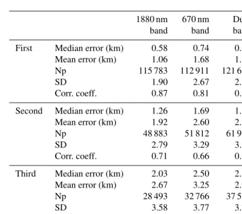
A summary of a baseline comparison between RSP and CPL, including the number of cases, median and mean differences, standard deviation and correlation coefficient, is given in Ta-ble 1. The comparison uses minimal filtering, namely only considering (a) RSP correlation peaks aggregated between 1.0 and 17.5 km in order to avoid interference by the surface or the aircraft; (b) peaks with a minimum correlation value of 0.1; and (c) second and third correlation peaks with at least 0.5 times the primary peak correlation value. All retrieved RSP layers are compared to the top of the closest CPL layer. The comparison uses data collected over eight flights of the SEAC4RS campaign.
Results for each of the wavelength bands show a gener-ally good agreement with the CPL observed heights. As seen in Table 1, the 1880 nm band’s primary peak gives the best agreement with CPL with a 0.58 km median error. The dual band gives similar results (0.61 km) along with the largest number of valid data points (121 679). The median error of the result using the 670 nm band is substantially larger at 0.74 km with 112 911 valid data points. All bands yield strong correlation coefficients for primary layer heights and reasonable values for secondary heights. Third-layer metrics are notably degraded for all bands. The dual band consis-tently yields the highest number of valid comparisons with a performance similar to that of the 1880 nm band.
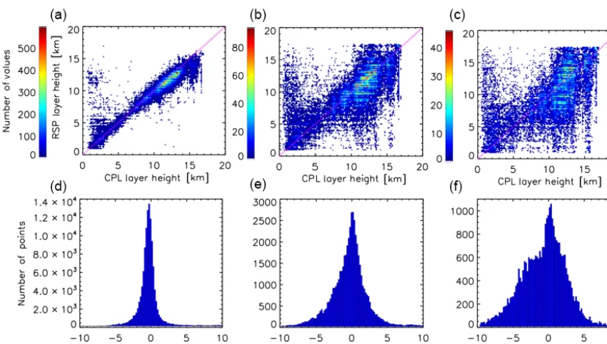
Figures 4–6 show direct comparisons of RSP-retrieved CTH for the first, second and third correlation peaks with the corresponding CPL layer top heights for the 1880 nm,
Table 1.Summary of baseline comparison.
1880 nm 670 nm Dual
band band band
First Median error (km) 0.58 0.74 0.61 Mean error (km) 1.06 1.68 1.22
Np 115 783 112 911 121 679
SD 1.90 2.67 2.14
Corr. coeff. 0.87 0.81 0.87
Second Median error (km) 1.26 1.69 1.30 Mean error (km) 1.92 2.60 2.28
Np 48 883 51 812 61 961
SD 2.79 3.29 3.25
Corr. coeff. 0.71 0.66 0.68
Third Median error (km) 2.03 2.50 2.10 Mean error (km) 2.67 3.25 2.92
Np 28 493 32 766 37 577
SD 3.58 3.77 3.70
Corr. coeff. 0.58 0.55 0.58
maxi-Figure 4.Comparison of CTH retrieved using the RSP 1880 nm band and CPL for the primary peak (top left), second peak (top middle) and third peak (top right) with their associated error distributions immediately below each scatterplot.
mum (FWHM) of the distribution is about 1.8 km. The com-parison for the CTH associated with the second correlation peak (Fig. 4b) has a similar shape but is more dispersed than the primary peak. This is apparent in the error distribution which is symmetrical, with little bias, but has a broader dis-tribution than that associated with the primary layer heights, with a FWHM of 3.4 km. The third peak (Fig. 4c) has a very similar spatial pattern as the second peak, but its error distri-bution (Fig. 4f) is no longer centered on zero bias, is more asymmetric and has a large FWHM of 7.5 km.
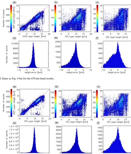
Similarly to Fig. 4, Fig. 5 shows the comparison of the re-sults using the 670 nm band with the CPL layer top heights. Again, the primary layer heights (Fig. 5a) agree well with the corresponding CPL heights, although there are a num-ber of cases where the CPL senses high-altitude clouds while the RSP’s 670 nm band detects low-lying features. This oc-curs when the CPL attenuates at a high altitude, but the RSP senses a strong low-lying feature. The higher feature may be distinguished in the 670 nm band’s second or third layer heights. The corresponding error distribution (Fig. 5d) shows a centered, narrow and symmetric distribution with a FWHM of 2.0 km, which is slightly broader than seen for the 1880 nm results (Fig. 4). However, there is a negative tail in the distri-bution resulting from the cases where RSP detects low-lying features while CPL detects higher clouds. The CTH compar-ison for the second correlation peak (Fig. 5b) shows good agreement between RSP and CPL CTHs, although the RSP senses many more low-lying features and because of this the error distribution (Fig. 5e) is asymmetric, with a negative off-set from center, and has a relatively large FWHM of 3.2 km.
The third peak (Fig. 5c) gives similar results to those found for the second peak, but the error distribution (Fig. 5f) has an even more pronounced asymmetry along with a very broad FWHM of 7.0 km.
Figure 6 shows the comparison of RSP’s dual band results to the closest CPL layer top heights. For the primary peak (Fig. 6a), good agreement is seen with points clustered along the 1 : 1 line along with two sets of outliers where the RSP senses high-altitude layers while the CPL senses low layers and vice versa. The error distribution (Fig. 6d) shows a nar-row peak nearly centered around zero and is symmetric. The FWHM of the distribution is 1.3 km. Again, the second and third peak comparisons are more dispersed, asymmetric and broader than the 1880 nm band results with FWHM values of 2.1 and 6.2 km, respectively. The dual band is included in our analysis with the aim of combining the strength of the 1880 band to sense high thin cirrus with the capability of the 670 nm band to retrieve the heights of lower layers. Compar-ing Fig. 6 to Figs. 4 and 5 shows that indeed the strengths of the two channels are well combined. However, the biases of the 1880 and 670 nm towards high and low layers, respec-tively, as compared to the CPL are also apparent in the dual band results.
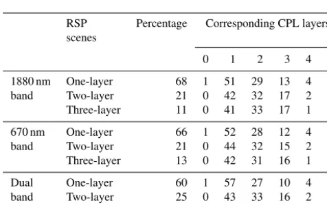
4.2 Number of cloud layers
Figure 5.Same as Fig. 4 but for the 670 nm band results.
Figure 6.Same as Fig. 4 but for the dual band results.
For example, for the 1880 nm band, RSP observes a single cloud layer 68 % of the time, and for these scenes the CPL sees a single layer 51 % of the time, while detecting multiple layers for 47 % of these cases. For only 1 % of these cases does CPL not detect any layers. Generally, cases with multi-ple cloud layers are seen by RSP at a rate of about 30–40 % of the time, with about double the probability of detecting two-layer scenes than three-layer ones. For these
Figure 7. (a)RSP CTH error and nadir template width for the 1880 nm band (blue), 670 nm band (green) and the dual band (red). The first, second and third layers are shown as stars, triangles and diamonds, respectively.(b)Absolute CTH difference and template variance.
Table 2.The 1880 nm band RSP cloud layer percentages compared with CPL.
RSP Percentage Corresponding CPL layers
scenes
0 1 2 3 4 5
1880 nm One-layer 68 1 51 29 13 4 1
band Two-layer 21 0 42 32 17 2 1
Three-layer 11 0 41 33 17 1 0
670 nm One-layer 66 1 52 28 12 4 1
band Two-layer 21 0 44 32 15 2 1
Three-layer 13 0 42 31 16 1 0
Dual One-layer 60 1 57 27 10 4 1
band Two-layer 25 0 43 33 16 2 1
Three-layer 15 0 40 33 17 2 1
thick clouds, while RSP can see below thick clouds because it is viewing them from the side but cannot see gaps within a single cloud layer. Overall, a similar performance is seen for all band configurations, although RSP results from the dual band agree somewhat better with the number of layers detected by CPL than results for the two single bands. 4.3 Nadir template attributes
Variation in intensity within the nadir template (R0)and the template width(NR)is an important aspect possibly affect-ing the correlation profile for a given pixel (Eq. 1). Figure 7a shows mean absolute error of each band as a function of the template pixel widthNR. An increase in error can be seen for each band when the template width is less than 9 pixels. The 1880 nm band’s error remains relatively constant for tem-plates of width 9 or more, but the dual band configuration ex-periences a slight decrease in error with increasing template width. For second and third layers, both the 670 nm band and 1880 nm bands experience increases in error with increas-ing template width. The dual band configuration shows an
overall reduction of error with increasing template width. For the analysis in this paper the template width is chosen to be 17. Based on Fig. 7a results are not expected to be substan-tially different when other template width are chosen. For a template width of 17, Fig. 7b shows how the variance of the 1880 nm band signal in the template is related to the accu-racy of the retrieval for the primary layer height. This shows the mean absolute error of the primary layers height for the 1880 nm band. It can be seen that there is a general decrease in error associated with increasing template variance, out to about 0.00012 in variance where the reduction in error lev-els off. A noticeable increase in error can be observed for the lowest value of variance where the error increases by about 300 m compared to the adjacent value.
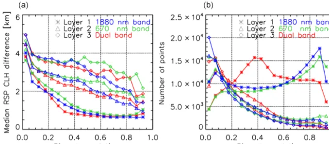
4.4 Correlation value
It is expected that the correlation strength of a given peak as calculated by Eq. (1) is related to the accuracy of the retrieved height. The effects of correlation value on the overall accu-racy of the approach is investigated here. All RSP-retrieved CTH’s between 1.0 and 17.5 km are considered. For layer CTHs detected using primary, second and third correlation peaks, Fig. 8a shows the accuracy for 0.05-wide bins of cor-relation values. Figure 8b shows the number of points that are included in each of the analyses.
uncer-Figure 8.RSP CTH error(a)and number of samples(b)versus the minimum correlation for the 1880 nm band (blue), 670 nm band (green) and the dual band (red). The first, second and third layers are shown as stars, triangles and diamonds, respectively.
tainty. Furthermore, filtering the results using a unique mini-mum correlation value for each of the peaks would improve the general level of accuracy, although at the cost of reducing the overall number of retrievals.
4.5 Cloud optical thickness
Here we investigate how the method performs for varying COTs. Passive sensors are typically less sensitive to optically thin clouds, so it is important to know the accuracy of the RSP’s ability to retrieve heights of clouds with low optical thicknesses. The CPL is capable of routinely sensing opti-cally thin clouds and is able to accurately sense multilayered cloud scenes up to a total optical thickness of about 3. How-ever, lidars are unable to sense cloud base of optically thick clouds or any clouds underneath. All of the comparisons start by using RSP-derived cloud heights; even as the layer opti-cal thicknesses decrease, comparisons are only done when the RSP senses a layer, and there are likely instances not re-flected in this assessment when CPL senses a thin layer that the RSP does not sense. For this part of the investigation, the baseline filtering described in Sect. 4.1 is used. Figure 9a shows the relation between the CPL optical thickness and the RSP cloud height error for all layers with calculated op-tical thicknesses. All bins are 0.25 wide except the last bin, which represents layers with optical thicknesses greater than 3.0. For the first layer, each of the bands’ errors remain rel-atively constant throughout the range of COTs even for lay-ers with an optical thickness below 0.1. If the RSP detects a layer, even of low optical thickness, it is consistent in its ability to determine the layer’s height. There are many cases where CPL senses two or more layers and the mode separa-tion difference is only 1 km, so it is possible that more than one CPL layer can be contributing to RSP’s retrieval. The errors have a slight, gradual increase with increasing optical thickness for the second and third layer. For clouds with op-tical thickness between 2.75 and 3.0, the difference between CPL and RSP heights is larger than for thinner clouds for
all bands and layers. This increased difference between CPL and RSP cloud heights near the saturation optical depth of the CPL may indicate that RSP detects layers below the satura-tion level of CPL. Interestingly, the difference between CPL and RSP heights is smaller again for CPL optical thicknesses above 3. In all cases, the number of points decreases expo-nentially up to an optical thickness of about 2.75 when more optically thick layers are observed, as seen in the right panel of Fig. 9.
4.6 Cloud top versus cloud middle
Passive sensors detect photons that have been scattered from a range of depths within a cloud’s diffuse boundary. In order to investigate to which depths within the cloud layers the re-trieved layer heights pertain, we present here a comparison of the RSP cloud layer heights using the 1880 nm, 670 nm and dual bands with the CPL’s cloud top and cloud mid-dle heights. This part of the analysis only considers clouds where the CPL can sense both a top and bottom and is there-fore limited to more tenuous clouds such that the CPL has not completely attenuated. Table 3 summarizes findings from the whole mission analysis.
Figure 9.RSP CTH error(a)and number of samples(b)versus CPL cloud optical thickness for the 1880 nm band (blue), 670 nm band (green) and the dual band (red). The first, second and third layers are shown as stars, triangles and diamonds, respectively.
Table 3.Summary of cloud top and cloud middle comparison.
1880 nm band 670 nm band Dual band
CPL cloud CPL cloud CPL cloud CPL cloud CPL cloud CPL cloud
top middle top middle top middle
First Median error (km) 0.58 0.42 0.74 0.54 0.61 0.45
Mean error (km) 1.05 0.86 1.69 1.41 1.21 0.98
Np 114 515 114 515 110 221 110 221 119 683 119 683
SD 1.86 1.73 2.67 2.57 2.12 2.01
Corr. coeff. 0.87 0.88 0.81 0.81 0.87 0.87
Second Median error (km) 1.26 1.19 1.69 1.52 1.30 1.18
Mean error (km) 1.92 1.80 2.60 2.36 2.28 2.09
Np 48 883 48 883 51 812 51 812 61 961 61 961
SD 2.79 2.67 3.29 3.19 3.25 3.14
Corr. coeff. 0.71 0.72 0.66 0.66 0.69 0.69
Third Median error (km) 2.03 1.98 2.50 2.35 2.10 1.99
Mean error (km) 2.67 2.55 3.25 3.02 2.92 2.72
Np 28 493 28 493 32 766 32 766 37 577 37 577
SD 3.58 3.45 3.77 3.67 3.70 3.56
Corr. coeff. 0.58 0.59 0.55 0.56 0.59 0.59
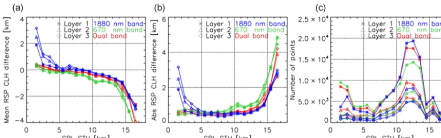
4.7 Error versus CTH
As apparent from Figs. 4–6, the accuracy of the retrieved CTHs depends on the CTH itself. This section examines how the retrieval error changes with cloud height. Figure 10a and b show the vertical distribution of mean and absolute dif-ferences, respectively, for each band’s first, second and third peaks against 1 km binned CPL heights. Figure 10c shows the number of points in each bin.
Figure 10a shows that the RSP consistently overestimates the height of low-lying clouds and underestimates the height of high clouds. Cloud top heights from about 14 to 17 km are underestimated in all cases. Qualitatively, the 1880 nm band largely overestimates the heights of clouds lower than 4 km, which is expected considering the reduced sensitivity of the
Figure 10.RSP mean error(a), absolute error(b)and number of clouds(c)versus CPL CTH.
4.8 Optimized performance example
Using the previous analyses, filters are implemented that use the strengths identified for each band. In Sect. 4.4, it was de-termined that in order to maximize the number of layer height retrievals, no minimum correlation threshold is used for the primary peak. Based on results shown in Fig. 7, for the sec-ond layer height, minimum correlation values of 0.3, 0.4 and 0.2 are chosen for the 1880 nm, 670 nm and dual band, re-spectively. For third-layer detection, minimum correlation of 0.5, 0.7 and 0.5 were chosen for the 1880 nm, 670 nm and dual band, respectively. This results in maximum errors of about 3 km for second and third layers for all bands. Based on results in Sect. 4.5, no minimum threshold on COT is im-plemented. According to findings shown in Sect. 4.6, the RSP CTH value is compared to CPL’s cloud middle for all bands. In cases where no cloud bottom is determined by CPL, the comparison is done to CPL cloud top. From Sect. 4.7, we restrict comparisons for the 1880 nm, 670 nm and dual bands to 4–17, 1–13 and 1–16 km, respectively. Table 4 summarizes the variables used for the 1880 nm, 670 nm and dual bands.
Using these values to filter layer detection, the median er-ror, mean erer-ror, number of points, standard deviation and cor-relation coefficient were calculated for each band over the eight flights used in this comparison and are summarized in Table 5.
Results for each of the bands show a better agreement with the CPL observed heights than the initial analysis shown in Table 1. In Table 5 it can be seen that the 1880 nm band has the lowest errors of 0.43, 1.35 and 1.96 for the first, second and third layers, respectively. Overall, the errors associated with the 1880 nm and dual band are similar, while the 670 nm band yields somewhat larger errors for each layer. Compared to values listed in Table 1, the primary layer retrieval shows the largest improvement with CTH biases that are reduced by 150–190 m (26 %) for each band. For the second and third layers for each band improvements are mainly appar-ent in the mean errors and standard deviation. In most cases, the primary and secondary layers retained nearly the same number of data points, while the third layer saw a
signifi-Table 4.Filters used for the optimal performance example.
1880 nm 670 nm Dual
Cloud top or middle Middle Middle Middle
Minimum COT 0.0 0.0 0.0
Minimum cloud height 4.0 km 1.0 km 1.0 km
Maximum cloud height 17.0 km 13.0 km 16.0 km
First peak minimum correlation 0.00 0.00 0.00
Second peak minimum correlation 0.30 0.40 0.20
Third peak minimum correlation 0.50 0.70 0.50
cant reduction in points used in each band due to the higher minimum correlation threshold. The correlation coefficients were either equal to the initial retrieval or reduced. Com-paring these results to other studies, MISR has been found to have an accuracy in detecting a single-layer CTH with a standard deviation of about 1 km when compared to MODIS and ground-based retrievals (Naud et al., 2007; Marchand et al., 2010). Naud et al. (2007) found the difference in CTH reduces to 0.35 km when only low-lying liquid clouds are considered. Mixed-phase clouds were found to have differ-ences of 0.4 km when compared to ground-based measure-ments above 5 km and 0.5 km when below 5 km. MISR- and MODIS-detected opaque ice clouds were found to have a difference of 0.3 km and cirrus clouds 1.2 km (Naud et al., 2007). Here, we show a high number of comparisons and observe similar results for the 1880 nm and dual band con-figurations and a lower accuracy for the 670 nm band.
Figure 11.Comparison of CTH retrieved using the RSP 1880 nm band and CPL for the primary peak (top left), second peak (top middle) and third peak (top right) with their associated error distributions immediately below each scatterplot. Here, filters detailed in Table 4 are applied.
Figure 12.Same as Fig. 11 but for the 670 nm band results.
of the results from 670 and dual band retrievals with CPL are less biased than results shown in Figs. 5 and 6, but the tails of the distributions remain.
Table 6 shows the average cloud heights over all eight flights obtained using each band and CPL, along with the mean and median cloud layer separation and number of
Figure 13.Same as Fig. 11 but for the dual band results.
Table 5.Summary of comparison with filters applied.
1880 nm 670 nm Dual
band band band
First Median error (km) 0.43 0.55 0.45 Mean error (km) 0.98 1.45 0.98
Np 109 369 105 783 121 372
SD 2.03 2.59 2.02
Corr. coeff. 0.78 0.79 0.87
Second Median error (km) 1.35 1.64 1.42 Mean error (km) 1.88 2.43 2.30
Np 44 851 30,257 67 863
SD 2.63 2.91 3.23
Corr. coeff. 0.59 0.59 0.63
Third Median error (km) 1.96 2.58 2.12 Mean error (km) 2.29 3.05 2.68
Np 12 858 6254 11 247
SD 2.90 2.87 3.13
Corr. coeff. 0.51 0.36 0.46
5 Conclusion
We presented a method of retrieving CTH using a multi-angular contrast approach that can be applied to every RSP footprint. The technique uses a cross-correlation calculation between multiple viewing angles corresponding to cloud lay-ers placed at specific altitudes. Local peaks in the calculated correlation profile as a function of height indicate the loca-tion of cloud layers. Multiple layers are identified by viewing
Table 6.Macro statistics.
1880 nm 670 nm Dual CPL band band band
Mean layer height (km) 10.74 7.58 9.00 9.47 Median separation (km) 2.10 1.90 2.50 2.67 Mean separation (km) 2.47 2.54 3.38 4.35
through optically thin layers. From this, we demonstrated the method’s capability of retrieving multiple cloud layer heights within a single RSP footprint.
The cloud height retrieval accuracies associated with the magnitude of the correlation metric, optical thickness and cloud height were explored. It was shown that each band maintained accuracy when retrieving cloud layer heights with very low optical thicknesses. It was found that RSP cloud layer height retrievals more accurately correspond to the CPL-derived cloud middle rather than cloud top. The 1880 nm band works best at middle and high altitudes (4.0 to 17 km), while the 670 nm band is best for low and mid-dle altitudes (1.0–13.0 km). A dual band configuration that combines 670 and 1880 nm measurement was found to be capable of retrieving cloud layer heights at altitudes between 1.0 and 16.0 km.
Data availability. The underlying RSP data used in this study are publicly available at https://data.giss.nasa.gov/pub/rsp/SEAC4RS/ (Cairns, 2013). The CPL data used in this study are publicly avail-able at https://cpl.gsfc.nasa.gov/ (McGill, 2013).
Competing interests. The authors declare that they have no conflict of interest.
Acknowledgements. Support for this work is provided by NASA grant no. NNX15AD44G (ROSES ACCDAM).
Edited by: A. Kokhanovsky
Reviewed by: three anonymous referees
References
Alexandrov, M. D., Cairns, B., Emde, C., Ackerman, A. S., and van Diedenhoven, B.: Accuracy assessments of cloud droplet size retrievals from polarized reflectance measurements by the research scanning polarimeter, Remote Sens. Environ., 125, 92– 111, 2012.
Alexandrov, M. D., Cairns, B., Wasilewski, A. P., Ackerman, A. S., McGill, M. J., Yorks, J. E., Hlavka, D. L., Platnick, S. E., Arnold, G. T., van Diedenhoven, B., Chowdhary, J., Ottaviani, M., and Knobelspiesse, K. D.: Liquid water cloud properties during the Polarimeter Definition Experiment (PODEX), Remote Sens. En-viron., 169, 20–36, 2015.
Alexandrov, M. D., Cairns, B., Van Diedenhoven, B., Ackerman, A. S., Wasilewski, A. P., McGill, M. J., Yorks, M. J. Hlavka, D. L., Platnick, S. E., and Arnold, G. T.: Polarized view of supercooled liquid water clouds, Remote Sens. Environ., 181, 96–110, 2016. Boucher, O., Randall, D., Artaxo, P., Bretherton, C., Feingold, G., Forster, P., Kerminen, V.-M., Kondo, Y., Liao, H., Lohmann, U., Rasch, P., Satheesh, S. K., Sherwood, S., Stevens, B., and Zhang, X. Y.: Clouds and Aerosols, in: Climate Change 2013: The Phys-ical Science Basis. Contribution of Working Group I to the Fifth Assessment Report of the Intergovernmental Panel on Climate Change, edited by: Stocker, T. F., Qin, D., Plattner, G.-K., Tig-nor, M., Allen, S. K., Boschung, J., Nauels, A., Xia, Y., Bex, V., and Midgley, P. M., Cambridge University Press, Cambridge, UK and New York, NY, USA, 2013.
Buriez, J. C., Vanbauce, C., Parol, F., Goloub, P., Herman, M., Bon-nel, B., Fouquart, Y., Couvert, P., and Seze, G.: Cloud detection and derivation of cloud properties from POLDER, Int. J. Remote Sens., 18, 2785–2813, 1997.
J. G., 207– 215, Blackwell Scientific Publishers, Oxford, UK, 1994.
Diner, D. J., Davies, R., Di Girolamo, L., Horvath, A., Moroney, C., Muller, J.-P., Paradise, S. R., Wenkert, D., and Zong, J.: MISR level 2 cloud detection and classification algorithm theoretical basis, Jet Propulsion Lab., JPL Tech. Doc. D-11399, Rev. D, Pasadena, CA, USA, 1999.
Fisher, D., Poulsen, C. A., Thomas, G. E., and Muller, J.-P.: Syn-ergy of stereo cloud top height and ORAC optimal estima-tion cloud retrieval: evaluaestima-tion and applicaestima-tion to AATSR, At-mos. Meas. Tech., 9, 909–928, https://doi.org/10.5194/amt-9-909-2016, 2016.
Lensky, I. M. and Rosenfeld, D.: The time-space exchangeability of satellite retrieved relations between cloud top temperature and particle effective radius, Atmos. Chem. Phys., 6, 2887–2894, https://doi.org/10.5194/acp-6-2887-2006, 2006.
Mace, G. G., Zhang, Q. Q., Vaughan, M., Marchand, R., Stephens, G., Trepte, C., and Winker, D.: A description of hydrometeor layer occurrence statistics derived from the first year of merged Cloudsat and CALIPSO data, J. Geophys. Res., 114, D00A26, https://doi.org/10.1029/2007JD009755, 2009.
Marchand, R., Ackerman, T., Smyth, M., and Rossow, W. B.: A review of cloud top height and optical depth histograms from MISR, ISCCP, and MODIS, J. Geophys. Res.-Atmos., 115, D16206, https://doi.org/10.1029/2009JD013422, 2010. Marchand, R. T., Ackerman, T. P., and Moroney, C.: An assessment
of Multiangle Imaging Spectroradiometer (MISR) stereo-derived cloud top heights and cloud top winds using ground-based radar, lidar, and microwave radiometers, J. Geophys. Res.-Atmos., 112, D06204, https://doi.org/10.1029/2006JD007091, 2007. McGill, M.: CPL SEAC4RS Campaign Data, NASA Goddad Space
Flight Center, available at: https://cpl.gsfc.nasa.gov/ (last access: 1 September 2016), 2013.
McGill, M., Hlavka, D., Hart, W., Scott, V. S., Spinhirne, J., and Schmid, B.: Cloud physics lidar: Instrument description and ini-tial measurement results, Appl. Optics, 41, 3725–3734, 2002. Menzel, W. P., Smith, W. L., and Stewart, T. R.: Improved cloud
motion wind vector and altitude assignment using VAS, J. Clim. Appl. Meteorol., 22, 377–384, 1983.
Menzel, W. P., Frey, R. A., Zhang, H., Wylie, D. P., Moeller, C. C., Holz, R. E., Maddux, B., Baum, B. A., Strabala, K. I., and Gumley, L. E.: MODIS global cloud-top pressure and amount estimation: Algorithm description and results, J. Appl. Meteorol. Clim., 47, 1175–1198, 2008.
Muller, J. P., Mandanayake, A., Moroney, C., Davies, R., Diner, D. J., and Paradise, S.: MISR stereoscopic image matchers: Tech-niques and results, IEEE T. Geosci. Remote, 40, 1547–1559, 2002.
Naud, C., Muller, J. P., and Clothiaux, E. E.: Compari-son of cloud top heights derived from MISR stereo and MODIS CO2-slicing, Geophys. Res. Lett., 29, 42-1–42-4, https://doi.org/10.1029/2002GL015460, 2002.
Naud, C. M., Baum, B. A., Pavolonis, M., Heidinger, A., Frey, R., and Zhang, H.: Comparison of MISR and MODIS cloud-top heights in the presence of cloud overlap, Remote Sens. Environ., 107, 200–210, 2007.
Rosenfeld, D., Woodley, W. L., Lerner, A., Kelman, G., and Lind-sey, D. T.: Satellite detection of severe convective storms by their retrieved vertical profiles of cloud particle effective radius and thermodynamic phase, J. Geophys. Res.-Atmos., 113, D04208, https://doi.org/10.1029/2007JD008600, 2008.
Toon, O. B., Maring, H., Dibb, J., Ferrare, R., Jacob, D. J., Jensen, E. J., Luo, Z. J., Mace, G. G., Pan, L. L., Pfister, L., Rosenlof, K. H., Redemann, J. S., Reid, J. S., Singh, H. B., Yokelson, R., Chen, G., Jucks, K. W., and Pszenny, A.: Planning, implementa-tion, and scientific goals of the Studies of Emissions and Atmo-spheric Composition, Clouds and Climate Coupling by Regional Surveys (SEAC4RS) field mission, J. Geophys. Res.-Atmos., 121, 4967–5009, https://doi.org/10.1002/2015JD024297, 2016. van Diedenhoven, B., Hasekamp, O. P., and Landgraf, J.: Retrieval
of cloud parameters from satellite-based reflectance measure-ments in the ultraviolet and the oxygen A-band, J. Geophys. Res., 112, D15208, https://doi.org/10.1029/2006JD008155, 2007. van Diedenhoven, B., Cairns, B., Fridlind, A. M., Ackerman, A.
S., and Garrett, T. J.: Remote sensing of ice crystal asymmetry parameter using multi-directional polarization measurements – Part 2: Application to the Research Scanning Polarimeter, At-mos. Chem. Phys., 13, 3185–3203, https://doi.org/10.5194/acp-13-3185-2013, 2013.
van Diedenhoven, B., Fridlind, A. M., Cairns, B., and Ackerman, A. S.: Variation of ice crystal size, shape, and asymmetry pa-rameter in tops of tropical deep convective clouds, J. Geophys. Res.-Atmos., 119, 11809–11825, 2014.
van Diedenhoven, B., Fridlind, A. M., Cairns, B., Ackerman, A. S., and Yorks, J.: Vertical variation of ice particle size in convective cloud tops, Geophys. Res. Lett., 43, 4586–4593, https://doi.org/10.1002/2016GL068548, 2016.
Wang, J. and Rossow, W. B.: Effects of cloud vertical structure on atmospheric circulation in the GISS GCM, J. Climate, 11, 3010– 3029, 1998.
Wang, J., Rossow, W. B., and Zhang, Y.: Cloud vertical structure and its variations from a 20-yr global rawinsonde dataset, J. Cli-mate, 13, 3041–3056, 2000.
Wind, G., Platnick, S., King, M. D., Hubanks, P. A., Pavolonis, M. J., Heidinger, A. K., Yang, P., and Baum, B. A.: Multilayer cloud detection with the MODIS near-infrared water vapor absorption band, J. Appl. Meteorol. Clim., 49, 2315–2333, 2010.
Wu, M. L. C.: Remote sensing of cloud-top pressure using reflected solar radiation in the oxygen A-band, J. Clim. Appl. Meteorol., 24, 539–546, 1985.