www.atmos-meas-tech.net/10/1893/2017/ doi:10.5194/amt-10-1893-2017
© Author(s) 2017. CC Attribution 3.0 License.
Pathfinder: applying graph theory to consistent tracking of daytime
mixed layer height with backscatter lidar
Marco de Bruine1,2, Arnoud Apituley1, David Patrick Donovan1, Hendrik Klein Baltink1, and Marijn Jorrit de Haij1 1Royal Netherlands Meteorological Institute (KNMI), Utrechtseweg 297, 3731 GA De Bilt, the Netherlands
2Institute for Marine and Atmospheric Research (IMAU), Utrecht University, Utrecht, the Netherlands
Correspondence to:Arnoud Apituley ([email protected])
Received: 3 October 2016 – Discussion started: 11 November 2016
Revised: 17 March 2017 – Accepted: 27 April 2017 – Published: 30 May 2017
Abstract. The height of the atmospheric boundary layer or mixing layer is an important parameter for understanding the dynamics of the atmosphere and the dispersion of trace gases and air pollution. The height of the mixing layer (MLH) can be retrieved, among other methods, from lidar or ceilometer backscatter data. These instruments use the vertical backscat-ter lidar signal to infer MLHL, which is feasible because the main sources of aerosols are situated at the surface and verti-cal gradients are expected to go from the aerosol loaded mix-ing layer close to the ground to the cleaner free atmosphere above. Various lidar/ceilometer algorithms are currently ap-plied, but accounting for MLH temporal development is not always well taken care of. As a result, MLHLretrievals may jump between different atmospheric layers, rather than reli-ably track true MLH development over time. This hampers the usefulness of MLHL time series, e.g. for process stud-ies, model validation/verification and climatology. Here, we introduce a new method “pathfinder”, which applies graph theory to simultaneously evaluate time frames that are con-sistent with scales of MLH dynamics, leading to coherent tracking of MLH. Starting from a grid of gradients in the backscatter profiles, MLH development is followed using Di-jkstra’s shortest path algorithm (Dijkstra, 1959). Locations of strong gradients are connected under the condition that subsequent points on the path are limited to a restricted ver-tical range. The search is further guided by rules based on the presence of clouds and residual layers. After being ap-plied to backscatter lidar data from Cabauw, excellent agree-ment is found with wind profiler retrievals for a 12-day pe-riod in 2008 (R2=0.90) and visual judgment of lidar data during a full year in 2010 (R2=0.96). These values com-pare favourably to other MLHLmethods applied to the same
lidar data set and corroborate more consistent MLH tracking by pathfinder.
1 Introduction
The atmospheric boundary layer is the lowest part of the at-mosphere where most of the interactions between surface and atmosphere take place. Knowledge of the processes and mechanisms in this layer is essential in meteorology and cli-mate science. The height of the boundary layer, or mixing layer height (MLH), is an important parameter; it affects, for example, near-surface air quality, since it limits the vol-ume of air into which pollutants are emitted, mixed and dis-persed, and is therefore crucial in modelling pollution, smog and dispersion of greenhouse gases. Since the height of the mixed layer is determined by surface fluxes that drive turbu-lent processes (Stull, 1988), it is one of the parameters that can be used to test model representation of the energy bal-ance against observations. MLH observations, therefore, are of key importance when testing models for a realistic rep-resentation of the atmosphere ranging from short timescales (weather forecasting) to long timescales (climate change).
installa-tions, due to the deployment in many national meteorological networks and at aerodromes (Thomas, 2016), and excellent temporal/spatial resolution – typically 24/7 coverage of tical profiles at time resolutions higher than 1 min and ver-tical resolutions of the order of 10 m. Data sampled at this resolution in time and space, assuming adequate signal to noise, should be sufficient to track MLH, which we intend to follow at a resolution of a couple of minutes and changes in the vertical of better than 100 m, which would be adequate for MLH studies.
Backscatter lidars and ceilometers are based on the same principles and use aerosol concentration as a tracer for MLH, which is possible because the main sources of aerosols are situated at the surface. The turbulent motions in the mix-ing layer cause the aerosol concentrations to be relatively well mixed within the layer, while exchange between mixing layer (ML) and free atmosphere (FA) is limited. As a result, higher aerosol concentrations are found within the mixing layer close to the ground and lower aerosol concentrations are found in the free atmosphere above. This difference in aerosol concentrations can be used to detect MLH.
Although the detection of the boundaries between atmo-spheric layers based on aerosol gradients has been used for many years, most of the backscatter-lidar-based techniques have difficulties to coherently track the MLH over time and may inadvertently jump between different atmospheric lay-ers, such as residual layers. Most algorithms search for the strongest gradient in a certain time window to which the MLH is then assigned, and the next time interval is treated in-dependently, with jumps between layers as a result. This lim-its the utility of these data records for deriving statistics and climatologies, as well as for processing studies and model validation/verification.
To alleviate this problem, guidance can be sought from an-cillary data (e.g. Pal et al., 2013). This improves MLH re-trieval at the cost of additional infrastructure and applicabil-ity will be limited to only those locations where the complete set of instruments is available. However, this also counteracts the attraction of the simplicity of the stand-alone backscat-ter lidar, which integrates these instruments into a network to monitor MLH over large, regional areas. Such approaches are discussed, e.g. in the COST action TOPROF (Illingworth, 2016), which aims to create an operational ground-based pro-filing with lidars and microwave radiometers for improving weather forecasts and E-PROFILE (EUMETNET, 2016) in which a framework is developed to exchange lidar backscat-ter data.
Here, we describe the new algorithm, pathfinder, which is used to track the development of the MLH during the day, based solely on single wavelength backscatter lidar data. The pathfinder algorithm is based on graph theory and the algo-rithm published by Dijkstra (1959) for finding the shortest path in graphs, and therefore inherently takes temporal de-velopment into account. Section 2 introduces the pathfinder method and gives a description of the different steps.
Sec-tion 3 describes different instruments used for boundary layer observations as well as the methods to derive MLH that are used in this paper for validation and verification. Section 4 presents results from this new method applied to data from Cabauw. The section is concluded with a sensitivity test.
2 Methodology
The most common techniques used to detect MLH from lidar measurements are the gradient method (e.g. Van Pul et al., 1994; Flamant et al., 1997; Menut et al., 1999), variance analysis (e.g. Hooper and Eloranta, 1986; Menut et al., 1999) and continuous wavelet transforms (e.g. de Haij et al., 2007). Doppler lidar techniques also use aerosol backscatter, but have additional information about the velocity of particles (Harvey et al., 2013).
These techniques evaluate measurements per time step in-dividually. Different features, like the residual layer and ad-vected aerosol layers can cause additional strong gradients in the lidar signal besides the MLH. These additional gradients can be of same order of magnitude as the backscatter gradi-ent on the MLH or even stronger, possibly leading to a MLH estimate alternating between these different layers. However, MLH is a relatively slowly evolving quantity and large dif-ferences between subsequent MLH estimates can be rejected. This can be accomplished by processing information from both the spatial and temporal domain simultaneously.
Alternatively, MLH can be determined manually. Even to-day, this remains a powerful way of determining MLH as the human brain can use knowledge on processes affecting ML development (e.g. time of sunrise and sunset or presence and type of clouds) to distinguish the correct MLH from other gradients. Plots of lidar RCS and gradient fields are visually inspected to determine exact MLH. Although this method does not give a completely independent validation for cor-rect MLH, it does provide an opportunity to assess the per-formance of the pathfinder method when applied to the same lidar measurements.
2.1 Input lidar data
The lidar data used are the range-corrected lidar signals (RCS). This is the signal that results after subtraction of the background sky light and correction of the z2 geometrical term in the lidar equation (e.g. Hinkley, 1976):
RCS(z)=z2P (z)
=z2·O(z)·β(z)·exp
−2 z Z
0
α(z0)dz0
, (1)
whereP (z)is the received power as function of distancez,
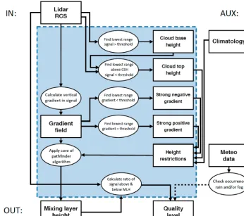
Figure 1.Flow diagram of the pathfinder algorithm. Internal operations and variables are grouped within the blue area. Input data are shown at the top and output variables at the bottom. Auxiliary data are displayed on the right. The use of collocated meteorological data is optional
area illuminated by the outgoing laser beam. For the MLH re-trieval, we will only be looking at the uncalibrated properties of the lidar signal, and in particular, the vertical gradient in RCS, indicated as RCS0. Calibration constants are therefore cancelled out. The overlap function, however, is important, as it increases from zero to unity from the ground up to the alti-tude of full overlap:zf. Abovezfwe assumeO(z > zf)=1. In the region of incomplete overlap below zf, RCS0 will be influenced by O by adding a systematic positive contribu-tion to the gradient. A further consequence of the lidar in-strument geometry is that no lidar signal is obtained at very close ranges below zb. In the lowest range between the in-strument andzb, the lidar is essentially blind.
2.2 The pathfinder method
The pathfinder method starts with a time series of RCS data as defined in Eq. 1, which is also represented in Fig. 3. Since the data can include atmospheric circumstances under which MLH detection may not be feasible (i.e. fog, intense precip-itation, low clouds), some pre-selection of data is needed, such as cloud screening. So first, parts of the data in time and/or height will be excluded for analysis based on four dif-ferent guiding restrictions as explained in Sect. 2.2.1. In the
second stage, as the core of the algorithm, the vertical gra-dients in the lidar data are computed and the gradient data RCS0are transformed into a mathematical graph in which all measurement points are represented by a node (vertex) and the connections (edges) are constructed based on costs calcu-lated from the measurements. Dijkstra’s (1959) algorithm is then applied to find the combination of measurement points representing the temporal evolution of the MLH. In the last stage a quality label is assigned to the MLH estimates based on the ratio of RCS above and below the MLH estimates. A flow diagram of the algorithm is given in Fig. 1.
2.2.1 Guiding restrictions
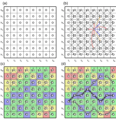
Figure 2.Overview of the translation of data into a mathematical graph and subsequent steps to determine MLH.(a)One-to-one translation of data points to graph vertices.(b)Grid of connections between vertices, for a single vertex allowed connections are shown in blue, examples of forbidden connections shown in orange and red. (c)Assignment of costs to the graph connections based on RCS vertical gradients. (d)Selection of correct path with Dijkstra’s algorithm, with three possible paths originating from the same point. Their total cost is displayed at the right. The middle path will be selected as the MLH development estimate as this is the path with the lowest possible cost.
The pathfinder algorithm restricts the maximum height of the MLH to the top of the first cloud layer. Cloud detection in pathfinder is simple yet effectively based on the magni-tude of RCS, which is possible due to the high backscat-ter on cloud droplets compared to aerosols. For each time step, the lowest altitude at which RCS exceeds a prescribed threshold is marked as cloud base height (CBH). After that, the lowest altitude above the CBH at which RCS drops be-low the same threshold is marked as cloud top height (CTH). Note that CTH is an apparent cloud top height. For optically thick clouds, the lidar signal might not penetrate the complete cloud and the signal might drop below the threshold value be-fore reaching the actual cloud top. Therebe-fore, it is not certain that CTH marks the correct cloud top. Nevertheless, we do
not limit the search range to the cloud base, because, in case of shallow cumulus clouds, the air in the cloud is part of the boundary layer. The apparent cloud top marked as CTH is al-ways closer to the correct cloud top and MLH than the cloud base.
Figure 3. (a)A full diurnal cycle of backscatter lidar profiles from the ALS450 system at Cabauw on 20 May 2010. The data presented are the range-corrected signal, RCS. The black line indicates pathfinder MLH solution.(b)The gradient field calculated from the backscatter lidar data.
morning, a stricter threshold can be used before the con-vective period. For an overview of thresholds used for the ALS450 UV-Lidar at Cabauw, see Table 2. To prevent exclu-sion of ML clouds, interaction between the positive gradient and previously described cloud detection is needed. When a cloud base is found within 300 m of a positive gradient, the search range is extended to the cloud top. This range is based on the typical scale of increased RH near clouds.
From literature, the scales associated with the ML in the midlatitudes are well known. For example, the ML in the Netherlands rarely extends above about 750 m during night-time and about 3000 m during daynight-time. This is implemented in the algorithm by restricting the search range during the morning period to that of the night period. On the onset of the convective period, a linear increase of 2.5 ms−1 is al-lowed, until the maximum altitude for daytime is reached. For the remainder of the day, the search range is limited by the daytime maximum.
Restriction to the exact altitude of cloud top or gradient might cause the exclusion of the actual MLH from the search range if the feature triggering a restriction is coincident with MLH. To prevent this from happening, the restrictions are relaxed in altitude by 75 m. Additionally, to prevent a sin-gle noisy measurement or inhomogeneity to disturb the algo-rithm, the restrictions are also relaxed in time by 2 min.
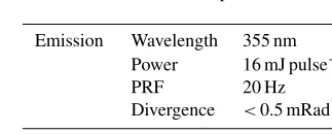
Table 1.Main characteristics of Leosphere ALS450.
Emission Wavelength 355 nm Power 16 mJ pulse−1 PRF 20 Hz Divergence <0.5 mRad
Detection Wavelength 355 nm
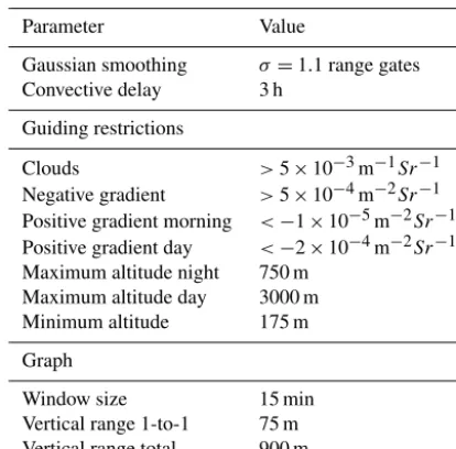
deter-Table 2.Overview of pathfinder parameters applied to Leosphere ALS450 lidar data.
Parameter Value
Gaussian smoothing σ=1.1 range gates Convective delay 3 h
Guiding restrictions
Clouds >5×10⁻³m−1Sr−1 Negative gradient >5×10⁻⁴m−2Sr−1 Positive gradient morning <−1×10⁻⁵m−2Sr−1 Positive gradient day <−2×10⁻⁴m−2Sr−1 Maximum altitude night 750 m
Maximum altitude day 3000 m Minimum altitude 175 m
Graph
Window size 15 min Vertical range 1-to-1 75 m Vertical range total 900 m
mined by the environment and referred to as “climatology” in the text.
2.2.2 Applying graphs
Tracking the evolution of MLH is essentially selecting a se-ries of points with corresponding time and altitude from a data set, based on certain criteria – much like planning an optimal route on a map. The mathematical representation of information in graphs is an excellent tool for this purpose. To apply graphs for MLH tracking from lidar measurements, we define the following four steps. First, a graph is set up with each point in the data set as vertices. Secondly, connections between these vertices are made so that any collection of con-nected vertices (hereafter called “path”) in the graph repre-sents a physically possible MLH evolution. Third, costs are assigned to the connections. Finally, the graph is searched by Dijkstra’s shortest path algorithm to select the optimal path following the MLH.
In the first step, a graph is created following the structure of the corresponding data set. Every point in the data set is translated into a vertex, regardless of the actual values in the data set. For a data set withNtime steps andMrange gates, this will lead to a graph withN×Mvertices, illustrated in Fig. 2a. In this stage, the graph is unstructured and the ver-tices unconnected.
To restrict possible paths in the graph to a physically sen-sible MLH evolution, connections between vertices repre-sent specific conditions. The first condition is that vertices only connect to vertices of the next time step. Connections to vertices of the same time step, previous time steps or more than one time step away are not allowed. These excluded connections are represented by the red arrows in Fig. 2b.
Next, only connections to vertices within a restricted ver-tical range are allowed – represented by the additional or-ange and blue arrows in Fig. 2b. The blue connections are allowed, but the orange connections are not because they ex-ceed the vertical range limit. Note that the representation in Fig. 2 is simplified and the actual vertical restriction can in-clude multiple range gates depending on the combination of vertical resolution of the data and chosen vertical restric-tion. In our implementation, the maximum allowed MLH growth rate is 2.5 ms−1, so the allowed range is 75 m when the time between measurements is 30 s. An additional re-striction is posed on a timescale of 15 min. Over this time window, connections to vertices exceeding a growth rate of 1 ms−1are not allowed. This growth rate is larger than val-ues found, e.g. by Baars et al. (2008), who reports valval-ues of 1 km h−1or 0.278 ms−1only in extreme cases. However, these values represent mean growth rates and do not repre-sent timescales resolving individual rising thermals. Imple-menting lower values caused problems in the pathfinder al-gorithm when tracking fast MLH development in the morn-ing.
In the third step, costs are assigned to the connections in the graph to determine which path represents the MLH from the collection created in the previous steps. For pathfinder, costsCare based on the vertical gradient RCS0:
C= − ∂
∂zRCS
−1
. (2)
Connections pointing to a certain vertex are assigned a cost corresponding to the point in RCS0represented by that ver-tex. Using this conversion, strong negative RCS0corresponds
to low costs and vice versa. Consequently, the path with the lowest total cost will include the vertices with strongest neg-ative gradients. The assignment of costs is shown in Fig. 2c, where the colours blue, green, yellow and red represent RCS0. Blue is the strongest negative gradient, green and yel-low are intermediate and red represents the weakest negative gradient. Note that the minus sign in the conversion Eq. (2) is needed for positive costs for negative gradients, since Di-jkstra’s algorithm needs positive costs. Whenever negative costs still occur, these are given a prescribed fill value.
In the final step, Dijkstra’s shortest path algorithm is ap-plied to select the optimal MLH path. This method efficiently determines the path with the lowest total cost originating from a specific vertex in the first time step to one of the vertices in the last time step satisfying the above-mentioned conditions (Fig. 2d).
method available for near-real-time MLH tracking. Whereas computational cost determines the upper limit of the window size, the lowest limit is determined by the typical timescale within the ML. For the results shown in Sect. 4, measure-ments are combined in time windows with a size of 15 min, which is large enough to capture several rising thermals si-multaneously. For a continuous series of MLH estimates, the last time step in a time window overlaps with the first time step of the subsequent time window. The MLH estimate in this time step is used as the starting point of the next time window. Without a preceding time window, the first win-dow on a day has no normal starting point. Instead, for the first time window the vertex in the first time step with the strongest negative gradient is used as the starting point. 2.2.3 Quality flagging
In the final stage of the pathfinder algorithm, a quality flag is added to each point of the MLH estimates. The quality criterion is based on the ratioRof the RCS above and below the estimated MLH, similar to the quality flag used in de Haij et al. (2007) and Morille et al. (2007). The ratio is calculated as follows:
rQ=
RCS(z=MLH,MLH+150 m)
RCS(z=MLH−150 m,MLH), (3)
where RCS indicates the average RCS over the indicated range interval.
Since we expect RCS to be smaller above MLH than below it,rQis expected to be less than 1. If the algorithm marked an erroneous, noise induced gradient within the ML or FA, the backscatter above and below the estimate are comparable and the ratio is close to 1. However, if the top of the residual layer is marked as MLH or aerosol concentrations in the ML as low, this ratio can also be small. Consequently, a high ratio is an indication of an incorrect MLH estimate, but a small ratio is no guarantee the MLH is correct. As a threshold, ratios above 0.9 are considered an indication of an incorrect MLH estimate.
3 Instrumentation 3.1 Cabauw site
The instruments for this study were located at the Cabauw Experimental Site for Atmospheric Research (CESAR; Apit-uley et al., 2008) in the Netherlands, where a suite of oper-ational and research mode remote sensing and in-situ mea-surements are performed to comprehensively characterise the atmospheric column. At CESAR, multiple instruments are operated that can be used to validate and verify the MLH re-trievals described here.
For the development of pathfinder, a continuous data set was needed from a backscatter lidar with sufficient signal
to noise. This was provided by the ALS450 described in Sect. 3.2. For comparison with other, independent, MLH methods (Sect. 3.3 and 3.4), periods were sought for, where multiple instruments were operating simultaneously. The in-struments and methods used are briefly introduced below.
3.2 Backscatter lidar
The main instrument used for the development and testing in this study was a single wavelength backscatter lidar, the Leo-sphere ALS450, operating at 355 nm. This particular instru-ment also measures depolarisation (Donovan and Apituley, 2013), but this information is not used here. The instrument is running 24/7 and records an averaged lidar signal every 30 s at a spatial resolution of 15 m. The ALS450 has a maximum operational vertical range for clouds and aerosols of 15 km during night-time and a reduced range of 8 km during the day due to remaining solar background. Main characteristics are tabulated in Table 1. The region of incomplete overlap between the probing laser beam and the receiving telescope extends up to about 500 m. All data from the ALS450 are available from the CESAR database (Baltink, 2016).
The atmospheric clear air attenuation is not entirely negli-gible at 355 nm, and adds a negative contribution to the gradi-ent. However, we will neglect contribution to the gradient, as it is very smooth compared to the gradients from the aerosol backscatter.
The ALS450 has been operational at Cabauw since 2007. Unfortunately, significant gaps exist in the instruments’ data record due to frequent instrument failure. The continuity of data coverage was best in 2010, which is why this data period was selected, providing a full annual cycle to be studied.
Also installed at Cabauw is an Impulsphysik LD40 ceilometer, which is part of the Dutch ceilometer network, from which MLH is routinely derived (de Haij et al., 2007). The LD40 operates at 905 nm and has a maximum opera-tional vertical range for clouds of about 10 km. However, for aerosols the range is often limited to 2 km or less due to the low signal-to-noise ratio (SNR). Pathfinder was applied to LD40 data, but due to the limited SNR no useful intercom-parison could be made to the ALS450 or other instruments. Currently, the LD40 is being decommissioned and replaced by the more capable Lufft CHM15k for the entire network in the Netherlands. However, the data could not be included in this study, but is the subject of future work.
3.3 Wind profiler
di-rections gives horizontal and vertical wind speeds. MLH de-tection from the wind profiler is possible since the intensity of the returning signal primarily depends on inhomogeneities in the atmospheric moisture and temperature caused by tur-bulence. The SNR is directly proportional to these inhomo-geneities, captured in the refractive index structure function
Cn2 (Ottersten, 1969). Due to the entrainment at the MLH,
Cn2exhibits a (local) maximum at this height. The width of the Doppler spectrum is also used in the MLH detection. The spectral width is related to the differences in wind speed in the probed volumes, is smaller in the entrainment layer than in the mixing layer itself and increases again into the free at-mosphere. Therefore, MLH is associated with a minimum in the spectral width. Results for the MLHW used in this paper use the method described by Angevine et al. (1994). A data set processed for MLH retrieval overlapping with ALS450 data was available for the IMPACT campaign in 2008 (Roelofs et al., 2010).
3.4 Radiosonde
Radiosonde data from Vaisala RS92-GDP measuring profiles of relative humidity, temperature, pressure and wind are used from the IMPACT campaign (Roelofs et al., 2010) that were launched from the Cabauw site. These sondes were used in the comparison between lidar, wind profiler and sonde (Sect. 4.3). Note that the sondes we used here for best col-location are not the routine radio sonde data from De Bilt, at about 20 km from Cabauw. However, for the full-year analy-sis presented in Sect. 4.4 we considered the De Bilt sondes.
Several methods exist to calculate MLH from the ra-diosonde measurements (MLHS), including the parcel method (Holzworth, 1964), lapse rate method (Hayden et al., 1997) and Richardson bulk method (Vogelezang and Holt-slag, 1996; Seibert et al., 2000). Here, we will use the Richardson bulk method since it takes into account both in-stability and wind shear.
4 Results
The performance of pathfinder is demonstrated in a couple of case studies: under clear-sky conditions in Sect. 4.1 and in more complex atmospheres with clouds and precipitation in Sect. 4.2. Subsequently, our new method is intercompared with MLH estimates from other instruments in Sect. 4.3. To test the applicability of pathfinder semi-operationally and to include a wide range of weather conditions, a comparison with manual MLH estimates for a full year is discussed.
Furthermore, the same data set is also processed by the STRAT2D method (Menut et al., 1999; Morille et al., 2007; Haeffelin et al., 2012) in Sect. 4.3.2. This method was se-lected, since the STRAT2D code has been made available to the community at large, specifically to be adapted and ap-plied to lidar instruments at the disposal of interested
inves-tigators. Therefore, pathfinder and STRAT2D applied to the same data provide an insight in algorithm differences, with-out introducing doubts abwith-out differences between various in-strument characteristics.
The following data are all based on measurements of the Leosphere ALS450 at Cabauw, for which the pathfinder tun-ing parameter values are listed in Table 2.
4.1 Clear sky
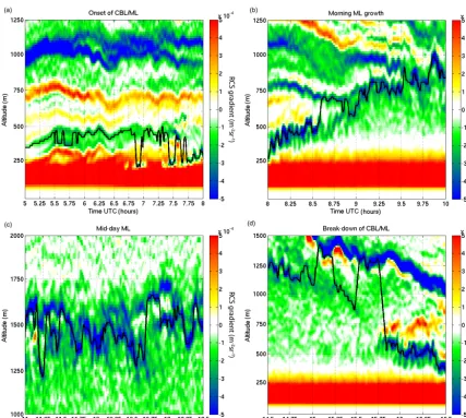
The first case study is the evolution of MLHL on 20 May 2010: a clear-sky day with a well-developed afternoon ML. The measured backscatter and corresponding vertical gra-dients are shown in Fig. 3. Also shown is the pathfinder MLH estimate from sunrise to sunset. To point out different features of the algorithm, four regions will be highlighted: (1) the period between sunrise and the onset of convection, (2) the morning growth of the ML, (3) the plateau during the middle of the day and (4) the breakdown of the ML and tran-sition into the night-time boundary layer. These regions can be seen in Fig. 4.
From sunset it takes several hours before the surface tem-perature is high enough to produce convection visible in lidar observations. With the complete ML below the lidar detec-tion rangezb, the solution tracks a gradient in stratification of the residual layer. Around 07:00 UTC, the ML rises above
zband becomes visible to the lidar. The solution indicates the correct altitude as MLH. As the layer moves up and down, it again sinks below the detectable range, but when the layer reappears after some 30 min, the solution again indicates the correct height for MLH.
The greatest challenge in deriving MLH from lidar mea-surements is to separate the gradient associated with the ML from the gradients in the residual layer. The pathfinder method will ignore additional layers when these are rela-tively far from the MLH. However, when an additional strong gradient exists close to the MLH, it might be included in the MLH estimate. The algorithms’ decision depends on the proximity of the gradients and the ratio of their relative strength. For the solution to shift to a different layer it has to transition several points of weak gradients and receives a penalty for this in the form of a higher path cost. A rela-tively strong gradient on a residual layer can outweigh this penalty and still cause a shift in the path with the lowest total path cost. Figure 4b shows that for the major part of the morning transition the correct MLH is indicated. Only around 08:45 UTC is the solution indeed triggered on a gra-dient in the residual layer, when the gragra-dient on the real MLH becomes weaker.
lim-Figure 4.Highlights of the MLH evolution at Cabauw on 20 May 2010. See text in Sect. 4.1. Gradients in RCS and pathfinder MLH estimates during a clear-sky day. These include(a)the period between sunrise and onset of the ML,(b)the morning growth of the ML,(c)the midday structure of the MLH and(d)the break-down of the ML. Time is indicated in decimal hours.
itation of 75 m between time steps is enough to follow the differences between thermals, such as the sudden decrease around 11:15 and 12:45 UTC.
4.2 Complex atmospheres
Even though a clear-sky day gives a good insight into differ-ent ML features, completely cloud-free days are scarce in the Netherlands. The presence of clouds influences the evolution of the ML (e.g. by blocking incoming solar radiation) and causes additional gradients which can distract the algorithm from the correct solution. As an example for this, the next case study treats a day with abundant fair-weather cumulus clouds. As can be seen in Fig. 5, two layers of clouds are present, mainly stratocumulus above cumulus clouds form-ing on top of the ML.
Around sunrise and sunset, the two cloud layers are well separated. Pathfinder correctly designates MLH to the top of
the lowest cloud layer. This is mainly due to the guiding re-striction that excludes measurements above the first cloud layer. However, this is a broken cloud deck and the guid-ing restrictions cannot exclude the stratocumulus clouds for all time steps. It is the combination of the guiding restriction together with the limited vertical search range that ensures correct tracking of the MLH even for broken cloud layers.
With the growth of the ML, the distance between the two cloud layers decreases up to a point where the two can no longer be distinguished when the signal extinction is too strong in the cumulus layer. During these periods, the solu-tion tracks the top of the stratocumulus as MLH, leading to short peaks in MLH, e.g. around 10:00 UTC.
Figure 5.Lidar RCS together with pathfinder MLH estimate on 11 April 2010. A day with cumulus cloud forming on top of the ML with an additional stratocumulus cloud layer above.
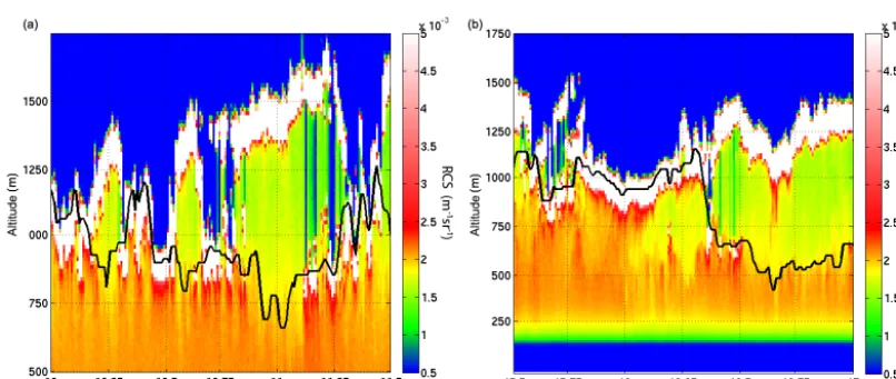
Figure 6.Highlights of the MLH estimate found by the pathfinder algorithm. See text in Sect. 4.2. Shown are(a)difficulties in distinguishing ML and non-ML clouds and(b)commitment to a cloud layer that detaches from the ML.
and 16:45 UTC. The ML decreases in depth, but the cloud layer remains at the same altitude. The pathfinder algorithm keeps tracking the strong gradients on the apparent cloud tops instead of the MLH. Because pathfinder is designed to track gradients close to adjacent gradients, the algorithm will not divert from a cloud layer until either strong gradients or clouds trigger the guiding rules.
The last two cases consider the ML during precipitation events. An example of a day with (heavy) precipitation is 8 June 2010, seen in Fig. 7. During and after precipitation, the lidar observations are affected by water on top of the in-strument. Only the strong backscatter on raindrops is strong enough to be distinguished from the background and noise. Therefore, a lidar-based MLH estimate in these periods is unreliable if not impossible. Between 06:30 and 08:30 UTC the estimates fluctuate between 150 and 750 m, the complete range allowed by the guiding restrictions. During rain be-tween 14:30 and 15:30 UTC, the signal is too low to calculate reliable MLH estimates.
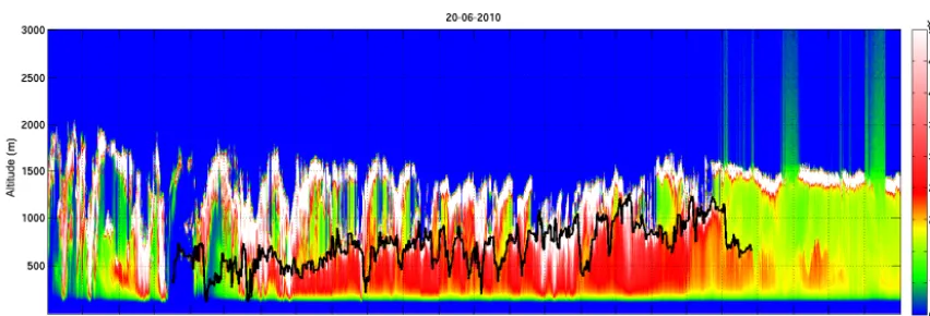
Another day with frequent precipitation is 20 June 2010, seen in Fig. 8. A characteristic of this day was that most of the precipitation evaporated before reaching the ground. Only 0.2 mm of rain was recorded at Cabauw that day. Without the observations affected by water on top the instrument, this day gives an insight into the effects of precipitation on the ML and the MLH solution of pathfinder under these condi-tions. Evaporating precipitation can be grouped into two cat-egories: evaporation in the lidar overlap region or well above it.
ap-Figure 7.Lidar RCS together with pathfinder MLH estimate on 8 June 2010. A day with varying cloud types and changing precipitation rates, including some showers between 06:00 and 09:00, 15:00 and 16:00 and at 19:00 UTC.
Figure 8.Lidar RCS together with pathfinder MLH estimate on 20 June 2010. A day with a completely overcast sky and precipitation falling from the cloud but (almost) completely evaporating before reaching the surface.
pears and with it the ML decreases in altitude. When the precipitation stops, air is no longer brought downward and the ML increases again in altitude. Under these conditions, the gradient on top of this layer is picked up well by the pathfinder algorithm. Similar events can be observed be-tween 11:45 and 12:00 or 12:30 and 13:00 UTC.
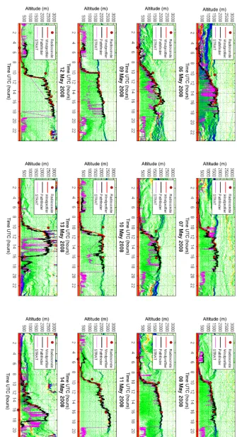
4.3 Comparison to other methods – 12-day period
For a comparison of the lidar methods, pathfinder and STRAT2D, which were applied to the same data, were com-pared to radiosonde and wind profiler MLH retrievals. We used the observations from a 12-day period in May 2008, ob-tained during the IMPACT campaign at Cabauw. Radiosonde observations were taken around 05:00, 10:00 and 16:00 UTC each day. The Richardson bulk method was used to esti-mate MLHR. The wind profiler operated continuously dur-ing IMPACT, but MLHW estimates could only be given for the above-mentioned 12-day period. The ALS450 also op-erated continuously and the pathfinder and STRAT2D algo-rithms were applied to derive MLH estimates, MLHL,P and
MLHL,S respectively. An overview of lidar measurements and the different MLH time series are shown in Fig. 10.
4.3.1 Wind profiler
The MLH estimates from the wind profiler and pathfinder algorithm are in excellent agreement, with 90 % of the pathfinder MLH estimates falling within a range of 250 m of the wind profiler values. Pathfinder mean bias compared to wind profiler MLH estimates is as small as−9.8 m. Largest deviations are found at midday. However, due to the differ-ence in approach and time resolution, it is not clear which MLH estimate is more correct. Next to that, pathfinder could not track the MLH on some of the mornings because the ML was too shallow and stayed under the detection range for a large part of the morning.
4.3.2 STRAT2D
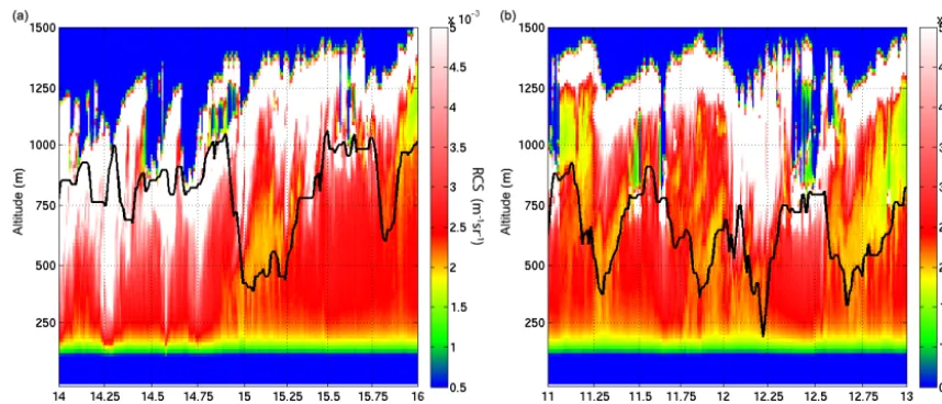
Figure 9.Highlights of the MLH estimate found by the pathfinder algorithm on 20 June 2010. See text in Sect. 4.2. Shown are(a)precipitation events reaching the lidar overlap region and(b)precipitation evaporating well above this region.
on a wavelet transform (Menut et al., 1999; Morille et al., 2007; Haeffelin et al., 2012). However, the main difference between the methods is in the ability to track the MLH over time, for which pathfinder introduces the use of graphs.
For large parts of the 12-day period, the estimates by STRAT2D and pathfinder agree well and also with the re-sults of the wind profiler. However, for STRAT2D large dif-ferences occur between subsequent time steps when irregu-larities are found within the ML. This leads to unrealistic, erratic estimates of MLHL,Sevolution during the day under some conditions. This behaviour is reflected in the mean bias of−244 m of STRAT2D compared to wind profiler MLH es-timates: 70 % of the STRAT2D estimates fall within a 250 m vertical range of wind profiler MLH estimates. Additionally, STRAT2D does not give an estimate due to the criterion that the ratio between backscatter above and below the MLH can-didate cannot exceed a prescribed value. During the IMPACT campaign, the ML air was relatively clean, yielding too low backscatter values in the ML compared to the free atmo-sphere in order to fulfill the STRAT2D criterion.
4.3.3 Radiosonde
Agreement between radiosonde and pathfinder strongly de-pends on the time of day. A good correlation (R2=0.88) is found for the 16:00 UTC soundings excluding 14 May, with a mean bias of only +18 m of pathfinder compared to ra-diosonde estimates and a RMSE of 156 m. By contrast, there is little agreement at 05:00 and 10:00 UTC. At 05:00 UTC, the ML is often too low to be detected by lidar and cannot be tracked by pathfinder. Comparing the 10:00 UTC soundings with the lidar observations, it becomes clear that the Richard-son bulk method often incorrectly designates the residual layer as MLH (e.g. 3, 10 and 12 May). This is reflected in a mean bias of−938 m of pathfinder MLH compared to
radiosonde estimates. An investigation of these 10:00 UTC soundings shows that a theoretical adiabatically rising air parcel indeed has positive buoyancy almost up to the ra-diosonde estimate. The Richardson bulk method estimates MLH slightly higher because wind shear is taken into ac-count. For 3 May, a well mixed-layer extending up to an alti-tude of 900 m can be distinguished from the radiosonde tem-perature profile (not shown), coinciding with the pathfinder MLH estimate. The Richardson bulk method, however, in-correctly estimates the MLH at about 1600 m. The reason may be that the Richardson bulk method does not take into account entrainment of environmental air into the rising ther-mal. By mixing in air with a lower (potential) temperature, the parcel loses its positive buoyancy at a lower altitude than the theoretical non-mixing rising parcel. Ignoring entrain-ment might be appropriate for deep convection, where the major part of the ascent takes place in non-turbulent air, but because of the turbulent nature of the ML, entrainment takes place at a much higher rate and cannot be neglected.
4.4 Full-year analysis of midday MLH
were used. Note that the pathfinder and visual/manual analy-sis have been performed on the exact same underlying instru-ment data. This ensures that only the algorithm is checked, without introducing new independent data.
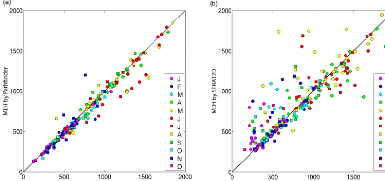
MLHM is compared to a 10 min average of MLHL,P around noon. The results are shown in Fig. 11a. The correla-tion with the manual estimates is as high asR2=0.90, mean bias of−50 m and a RMSE of 83 m. If the pathfinder quality criterion is used, which identifies estimates where the ratio between backscatter below and above the candidate MLHL,P (i.e. RCS(z >MLHL,P)/RCS(z <MLHL,P)) is larger than 0.9, a number of days are excluded, and 197 days remain where confidence is highest. This data set yields a correlation between MLHM and MLHL,P of R2=0.95, with a mean bias of −30 m and RMSE of 61 m. The STRAT2D results were also compared to the manual estimates. STRAT2D only gives an estimate if the same quality criterion is used, which leaves 234 days with a correlation ofR2=0.74, mean bias of +43 m and a RMSE of 127 m. The scatter that is larger than the pathfinder is apparent in Fig. 11b. Most of the mis-matches are caused by an overestimation of the MLH by STRAT2D. In these cases STRAT2D designates the top of the residual layer as MLH. The colour coding in Fig. 11 in-dicates the month and reveals the seasonality. As expected, lowest MLH estimates are found in winter and highest esti-mates in spring and summer.
4.5 Parameter sensitivity
Pathfinder limits the search for MLH to altitudes near pre-viously found MLH estimates, which gives it its improved tracking behaviour. However, the method may be sensitive to initialisation parameters. Two parameters in particular that may have an effect on the retrieved MLHL,P time series are the start time on the day of the first time step and the time window size, i.e. the number of time steps treated simultane-ously. When two possible paths have comparable total cost, including or excluding time steps in a time window might tip the outcome to either one of those competing paths. This would change the MLH estimate of that time window and possibly the outcome of subsequent time windows.
4.5.1 Variation of the initial start time
A change in the position of the first time step will not change the size of the search range, but shifts it along the time axis together with all other time windows of that day. As a conse-quence, the first MLH candidate found may be different from the one found in the default run and this may influence the subsequent MLH estimates since they are bound to the pre-vious MLH estimates. The default time window is 15 min, i.e. 30 time steps for the ALS450. In the test, the time win-dow was shifted forward and backward by 1 to 30 time steps, leading to a total of one base plus 60 sensitivity runs for each day considered. The analysis was applied to the observations
of May 2010. Overall, very high agreement between base and sensitivity runs is found. There is an exact agreement at least 93.1 % for all individual time steps of the complete month when comparing the results of one sensitivity run with the base case. Accompanying mean bias is as low as 4.15 m and maximum monthly mean RMSE of 17 m. As expected, agreement deteriorates when start and endpoints of the time windows go further away from their original position in the base run. Lowest agreement is found for a forward shift of 17 time steps.
4.5.2 Extent of the search time window
Within a time window, the vertical search range increases with 75 m both upward and downward each time step with our current settings. If the window size is increased, the search range consequently expands and more measurements are included in the search.
Next to the default time window of 30 time steps, calcu-lations are made for window sizes between 10 and 70 time steps with increments of 10 time steps. Again, the ALS450 observations from May 2010 were used. Again, the algo-rithm showed stable behaviour and the exact same solution is found between 95.3 and 96.6 % of the individual time steps in the month when using time windows between 20 and 70 time steps. Corresponding mean bias ranges between−7.0 and+0.5 m and RMSE between 12.5 and 15.3 m. The per-formance for a window size of 10 time steps was slightly worse with an exact match of 89.6 %, mean bias of−21.7 m and RMSE of 34 m. For this smallest time window, the maxi-mum allowed change of the MLH of 1 ms−1between starting and endpoint of the time window caused the algorithm to be unable to correctly track differences between individual ris-ing thermals. As a result, many short-term differences occur between these runs and the default calculations.
All sensitivity runs with a larger time window showed the lowest correlations for a single day all on 27 May. Apart from some exceptions, this was due to the period between 14:00 and 16:00 UTC when a residual layer with clouds was in close proximity to the MLH. For window sizes larger than 30 time steps, the solution jumped from the MLH to a residual layer and followed this layer between 14:00 and 16:00 UTC. Runs with a smaller window size tracked MLH during the whole period. Pathfinder has to include several high cost time steps to allow for a jump to another layer. For relatively small time windows, there are not enough time steps left to com-pensate for this extra cost and the jump is rejected as a so-lution. In case of larger time windows, this might not be the case and the solution is allowed to jump to another layer more easily. This divergence continues as long as the tracked fea-ture (e.g. residual or cloud layer) exists or the guiding re-strictions pick up gradients forcing the calculations back to the correct solution.
Figure 11.Scatter plots of(a)pathfinder MLHL,P against MLHM (R2=0.96) and(b)STRAT2D MLHL,S against MLHM (R2=0.74) for the full data set of 2010. Colour coding indicates the month of the year.
MLH estimates during a day irrespective of the time window settings. Although solutions can diverge for short periods, the guiding restrictions force the calculations back to the correct solution.
4.6 Discussion
The clear-sky cases show that the guiding restrictions suc-cessfully exclude large parts of the additional gradients of the residual layer. This prevents the need to apply strong smoothing filters or averaging and allows the shortest path algorithm to determine the evolution of the MLH on the na-tive resolution of the underlying data. In case the guiding restrictions do not exclude all additional gradients, a jump to another layer of high gradients is most often prevented by the shortest path algorithm itself. For a transition, several mea-surement points with low gradients have to be included in the path, increasing the total cost of the jump. A transition can-not always be prevented if the additional gradients are strong enough to compensate for the extra cost. Here, further study would be needed on how to tune the algorithm settings. Also, atmospheric conditions that are different from the Dutch con-ditions may require different settings.
Clouds can be a good indicator of MLH height, but the high backscatter on the cloud droplets cause a negative gra-dient typically an order of magnitude larger than gragra-dients associated with differences in aerosol concentration. Because of these strong gradients, the solution found by the algorithm is drawn to cloud tops. In case of a cloud layer above the ML, guidance is needed to restrict the algorithm to the MLH, for instance, by a more rigorous cloud screening prior to the pathfinder analysis.
During rain MLHL,P derivation is difficult, because of the attenuation of the lidar signal. If precipitation did not reach the surface, it could be seen that the downdraught of a rain
shower lowered MLH. Pathfinder is able to correctly follow this decrease in MLH as long as the precipitation evaporates above the overlap regionzf, otherwise there is no negative gradient to assign MLHL,P to. The top of the precipitating cloud will be marked as MLHL,P instead, although it is not the actual MLH.
Because of the high temporal resolution of the lidar obser-vations, changes in MLH by individual thermals are domi-nant. The typical spatial scale of the thermals is of the order of several hundreds of metres up to a kilometre. To compare results to other instruments with a similar time resolution, their collocation should be better than this typical scale.
Since the MLH at night in the Netherlands is often be-low the minimum overlap region of the ALS450 used in this study, no attempts were made to derive the nocturnal bound-ary layer. Nocturnal boundbound-ary layers could be tracked if the lidar profiles would start at appropriately low heights.
Whereas pathfinder was developed specifically for MLH retrieval from stand-alone single wavelength backscatter li-dar data, the method may be generalised to be applied to data from other profiling instruments for MLH retrieval. More-over, pathfinder may be embedded in a chain of multiple al-gorithms, such as cloud screening. One such example has re-cently been described by Poltera et al. (2017).
5 Conclusions
individual to visually recognise the MLH development in li-dar RCS plots. To accommodate for this, a new method was proposed called “pathfinder”. This method evaluates multi-ple time steps within a configurable time window simultane-ously. Graph theory is applied together with Dijkstra’s short-est path algorithm (Dijkstra, 1959) to imitate the continuous character of the MLH.
The pathfinder algorithm stores a full day of lidar mea-surements arranged in a time–altitude matrix and subse-quently divides the matrix into time windows of 15 min. These 15 min blocks are translated into graphs in which each individual data point represents a vertex. To estimate MLH exactly one altitude has to be selected in each time step. For the selection a certain cost is assigned to each vertex, which is inversely proportional to the gradient at the point in the graph. This way, the path with the lowest total cost will contain the maximum sum of strong gradients and will be a good estimate for the MLH. To mimic the gradual evolu-tion of the MLH, the distance between subsequent points is restricted. The threshold used for this is a maximum growth rate of 2.5 ms−1. Between the first and last time steps of a time window, this threshold is lowered to 1 ms−1. To guide the shortest path algorithm, a set of rules is used. Features like clouds, strong negative and positive gradients exclude parts of the observations from the search range for MLH.
Pathfinder was applied to data from a Leosphere ALS450 deployed at the Cabauw Experimental Site (CESAR) in the Netherlands. The results were checked against MLH esti-mates obtained from independent observations, such as those from a wind profiler and radiosondes. Excellent agreement was found between MLH estimates of the pathfinder method and from the wind profiler during a 12-day period (IMPACT campaign, May 2008). The comparison with collocated ra-diosonde data was more problematic, we believe, due to lim-itations in the Richardson bulk method. Pathfinder results were also checked against manual/visual MLH retrieval ap-plied to the same data, as well as the results from a different algorithm, STRAT2D, applied to the same data.
In in this study, pathfinder gives less scatter than STRAT2D in the comparison of a full-year analysis with manual MLH retrievals. This is due to the jumps between layers present in the STRAT2D estimates.
The pathfinder method can be used operationally on stand-alone single wavelength backscatter lidar data, provided the signal-to-noise ratio is sufficient to detect aerosol layers up to a few kilometres above ground. The typical computation time is less than 5 min for observations from a full day, based on the Leosphere ALS450 data set. An application of pathfinder to other lidar instruments, such as the Lufft CHM15k which now being deployed in the Dutch operational observation network, is currently under investigation.
Data availability. The lidar data used in this study are publicly available from the CESAR database http://www.cesar-database.nl.
Competing interests. The authors declare that they have no conflict of interest.
Acknowledgements. The authors thank the STRAT development team for making the STRAT2D code available, for their support and fruitful discussions. The authors also thank the reviewers for their positive comments and feedback, which made it possible to improve and clarify the paper.
Edited by: L. Bianco
Reviewed by: W. Angevine and one anonymous referee
References
Angevine, W. M., White, A. B., and Avery, S. K.: Boundary-layer depth and entrainment zone characterization with a boundary-layer profiler, Bound.-Lay. Meteorol., 68, 375–385, doi:10.1007/BF00706797, 1994.
Apituley, A., Russchenberg, H., van der Marel, H., Boers, R., ten Brink, H., de Leeuw, G., Uijlenhoet, R., Arbresser-Rastburg, B., and Röckmann, T.: Overview Of Research And Networking With Ground Based Remote Sensing For Atmospheric Profiling At The Cabauw Experimental Site For Atmospheric Research (CESAR) – The Netherlands, in: Proceedings IGARSS 2008, Boston, Massachusetts, III, 903–906, 2008.
Baars, H., Ansmann, A., Engelmann, R., and Althausen, D.: Con-tinuous monitoring of the boundary-layer top with lidar, At-mos. Chem. Phys., 8, 7281–7296, doi:10.5194/acp-8-7281-2008, 2008.
Baltink, H. K.: CESAR-database, available at: http://www. cesar-database.nl (last access: 25 May 2017), 2016.
Beyrich, F.: Mixing-height estimation in the convective bound-ary layer using sodar data, Bound.-Lay. Meteorol., 74, 1–18, doi:10.1007/BF00715708, 1995.
de Haij, M., Wauben, W., and Baltink, H. K.: Continuous mixing layer height determination using the LD-40 ceilometer: a feasi-bility study, Scientific report 2007-01, KNMI, De Bilt, 102 pp., 2007.
Dijkstra, E. W.: A note on two problems in connexion with graphs, Numer. Math., 1, 269–271, doi:10.1007/BF01386390, 1959. Donovan, D. P. and Apituley, A.: Practical
depolarization-ratio-based inversion procedure: lidar measurements of the Eyjafjal-lajökull ash cloud over the Netherlands, Appl. Opt., 52, 2394– 2415, doi:10.1364/AO.52.002394, 2013.
Eresmaa, N., Karppinen, A., Joffre, S. M., Räsänen, J., and Talvitie, H.: Mixing height determination by ceilometer, Atmos. Chem. Phys., 6, 1485–1493, doi:10.5194/acp-6-1485-2006, 2006. EUMETNET: E-PROFILE Website, available at: http://www.
eumetnet.eu/e-profile (last access: 25 May 2017), 2016. Flamant, C., Pelon, J., Flamant, P. H., and Durand, P.: Lidar
de-termination of the entrainment zone thickness at the top of the unstable marine atmospheric boundary layer, Bound.-Lay. Mete-orol., 83, 247–284, doi:10.1023/A:1000258318944, 1997. Haeffelin, M., Angelini, F., Morille, Y., Martucci, G., Frey, S.,
Ceilome-ters in View of Future Integrated Networks in Europe, Bound.-Lay. Meteorol., 143, 49–75, doi:10.1007/s10546-011-9643-z, 2012.
Harvey, N. J., Hogan, R. J., and Dacre, H. F.: A method to diagnose boundary-layer type using Doppler lidar, Q. J. Roy. Meteorol. Soc., 139, 1681–1693, doi:10.1002/qj.2068, 2013.
Hayden, K., Anlauf, K., Hoff, R., Strapp, J., Bottenheim, J., Wiebe, H., Froude, F., Martin, J., Steyn, D., and McKendry, I.: The verti-cal chemiverti-cal and meteorologiverti-cal structure of the boundary layer in the Lower Fraser Valley during Pacific ’93, Atmos. Environ., 31, 2089–2105, doi:10.1016/S1352-2310(96)00300-7, 1997. Hinkley, E. D.: Laser monitoring of the atmosphere, Springer
Ver-lag, Berlin, 1976.
Holzworth, G. C.: Estimates of mean maximum mixing depths in the contiguous United States, Mon. Weather Rev, 92, 235–242, 1964.
Hooper, W. P. and Eloranta, E. W.: Lidar Measurements of Wind in the Planetary Boundary Layer: The Method, Accuracy and Results from Joint Measurements with Radiosonde and Kytoon, J. Climate Appl. Meteorol., 25, 990–1001, doi:10.1175/1520-0450(1986)025<0990:LMOWIT>2.0.CO;2, 1986.
Illingworth, A.: TOPROF website, available at: http://www.toprof. imaa.cnr.it (last access: 25 May 2017), 2016.
Menut, L., Flamant, C., Pelon, J., and Flamant, P. H.: Ur-ban boundary-layer height determination from lidar mea-surements over the Paris area, Appl. Opt., 38, 945–954, doi:10.1364/AO.38.000945, 1999.
Morille, Y., Haeffelin, M., Drobinski, P., and Pelon, J.: STRAT: An Automated Algorithm to Retrieve the Vertical Structure of the Atmosphere from Single-Channel Lidar Data, J. Atmos. Ocean. Technol., 24, 761–775, doi:10.1175/JTECH2008.1, 2007. Ottersten, H.: Atmospheric Structure and Radar
Backscat-tering in Clear Air, Radio Sci., 4, 1179–1193, doi:10.1029/RS004i012p01179, 1969.
Pal, S., Haeffelin, M., and Batchvarova, E.: Exploring a geophysical process-based attribution technique for the determination of the atmospheric boundary layer depth using aerosol lidar and near-surface meteorological measurements, J. Geophys. Res.-Atmos., 118, 9277–9295, doi:10.1002/jgrd.50710, 2013.
Poltera, Y., Martucci, G., Collaud Coen, M., Hervo, M., Emmeneg-ger, L., Henne, S., Brunner, D., and Haefele, A.: Pathfinder-TURB: an automatic boundary layer algorithm. Development, validation and application to study the impact on in-situ mea-surements at the Jungfraujoch, Atmos. Chem. Phys. Discuss., doi:10.5194/acp-2016-962, in review, 2017.
Roelofs, G.-J., ten Brink, H., Kiendler-Scharr, A., de Leeuw, G., Mensah, A., Minikin, A., and Otjes, R.: Evaluation of simulated aerosol properties with the aerosol-climate model ECHAM5-HAM using observations from the IMPACT field campaign, At-mos. Chem. Phys., 10, 7709–7722, doi:10.5194/acp-10-7709-2010, 2010.
Seibert, P., Beyrich, F., Gryning, S.-E., Joffre, S., Rasmussen, A., and Tercier, P.: Review and intercomparison of operational meth-ods for the determination of the mixing height, Atmos. Environ., 34, 1001– 1027, doi:10.1016/S1352-2310(99)00349-0, 2000. Stull, R.: An Introduction to Boundary Layer Meteorology,
Springer, 1988.
Thomas, W.: DWD Ceilometer Map, available at: http://dwd.de/ ceilomap (last access: 25 May 2017), 2016.
Van Pul, W. A. J., Holtslag, A. A. M., and Swart, D. P. J.: A comparison of ABL heights inferred routinely from lidar and radiosondes at noontime, Bound.-Lay. Meteorol., 68, 173–191, doi:10.1007/BF00712670, 1994.
Vogelezang, D. H. P. and Holtslag, A. A. M.: Evaluation and model impacts of alternative boundary-layer height formulations, Bound.-Lay. Meteorol., 81, 245–269, doi:10.1007/BF02430331, 1996.
Wiegner, M., Emeis, S., Freudenthaler, V., Heese, B., Junkermann, W., Münkel, C., Schäfer, K., Seefeldner, M., and Vogt, S.: Mix-ing layer height over Munich, Germany: Variability and compar-isons of different methodologies, J. Geophys. Res.-Atmos., 111, doi:10.1029/2005JD006593, 2006.