www.atmos-meas-tech.net/8/4155/2015/ doi:10.5194/amt-8-4155-2015
© Author(s) 2015. CC Attribution 3.0 License.
APOLLO_NG – a probabilistic interpretation of the APOLLO
legacy for AVHRR heritage channels
L. Klüser, N. Killius, and G. Gesell
German Aerospace Center, German Remote Sensing Data Center, Oberpfaffenhofen, Weßling, Germany Correspondence to: L. Klüser ([email protected])
Received: 19 March 2015 – Published in Atmos. Meas. Tech. Discuss.: 30 April 2015 Revised: 30 September 2015 – Accepted: 30 September 2015 – Published: 12 October 2015
Abstract. The cloud processing scheme APOLLO (AVHRR Processing scheme Over cLouds, Land and Ocean) has been in use for cloud detection and cloud property re-trieval since the late 1980s. The physics of the APOLLO scheme still build the backbone of a range of cloud detec-tion algorithms for AVHRR (Advanced Very High Resolu-tion Radiometer) heritage instruments. The APOLLO_NG (APOLLO_NextGeneration) cloud processing scheme is a probabilistic interpretation of the original APOLLO method. It builds upon the physical principles that have served well in the original APOLLO scheme. Nevertheless, a couple of additional variables have been introduced in APOLLO_NG. Cloud detection is no longer performed as a binary yes/no decision based on these physical principles. It is rather ex-pressed as cloud probability for each satellite pixel. Con-sequently, the outcome of the algorithm can be tuned from being sure to reliably identify clear pixels to conditions of reliably identifying definitely cloudy pixels, depending on the purpose. The probabilistic approach allows retrieving not only the cloud properties (optical depth, effective radius, cloud top temperature and cloud water path) but also their un-certainties. APOLLO_NG is designed as a standalone cloud retrieval method robust enough for operational near-realtime use and for application to large amounts of historical satellite data. The radiative transfer solution is approximated by the same two-stream approach which also had been used for the original APOLLO. This allows the algorithm to be applied to a wide range of sensors without the necessity of sensor-specific tuning. Moreover it allows for online calculation of the radiative transfer (i.e., within the retrieval algorithm) giv-ing rise to a detailed probabilistic treatment of cloud vari-ables. This study presents the algorithm for cloud detection and cloud property retrieval together with the physical
prin-ciples from the APOLLO legacy it is based on. Furthermore a couple of example results from NOAA-18 are presented.
1 Introduction
During all these years of research with use of APOLLO a couple of limitations have been identified. Oumbe et al. (2013) propose to retrieve cloud effective radius together with the optical depth estimation in order to improve the modeling of cloud extinction for solar irradiance calcula-tions. Klüser and Holzer-Popp (2010) reported that the lack of cloud effective radius retrieval is very disadvantageous in aerosol-cloud-interaction studies. Merchant et al. (2005) point out the advantage of a more flexible probabilistic cloud detection scheme. The same argument is brought by Holzer-Popp et al. (2013) with a different focus: in comparing cloud masks from the aerosol_cci and the cloud_cci projects they found that about 20 % of all observations were used nei-ther for aerosol retrieval nor for cloud retrieval. The reason outlined in Holzer-Popp et al. (2013) was that aerosol re-trievals require a cloud mask which is precise about clear-sky pixels (a so called clear-conservative cloud mask). On the other hand, for retrieving cloud properties it is necessary to be sure that the pixel is cloudy (cloud-conservative cloud mask). Consequently, there is no single cloud mask fulfill-ing the need of both groups. Cloud detection has thus to be flexible with respect to the application it is used for.
Different versions of the APOLLO algorithm have evolved over time (e.g., Kriebel et al., 2003; Holzer-Popp et al., 2008; Klüser and Schepanski, 2009; Klüser and Holzer-Popp, 2010). The evolution of varying versions for different purposes and sensors made it desirable to harmonize the sen-sor dependent versions again. Necessary requirements like the introduction of a cloud droplet effective radius retrieval along with the optical depth estimation (Nakajima and King, 1990), the use of modern representations of ice cloud optical properties (Baum et al., 2014) and the requirement for more flexible cloud detection (Merchant et al., 2005; Holzer-Popp et al., 2013) consequently motivated the development of a new cloud detection and cloud retrieval scheme based on the physical principles of APOLLO.
As a direct consequence, a new probabilistic cloud de-tection scheme has been developed from the basis of the APOLLO physics. One major goal of the next generation method is to be applicable with any satellite sensor provid-ing the traditional five AVHRR channels (centered approx-imately at 0.6, 0.9, 1.6/3.7, 11 and 12 µm). Consequently, the new scheme does not use additional channels (like those centered at 8.7 or 13.4 µm), which are available on instru-ments such as SEVIRI or the new Visible Infrared Imag-ing Radiometer Suite (VIIRS) onboard the recently launched Suomi satellite. The probabilistic scheme still relies on the same physical assumptions as the original APOLLO scheme. The scheme is specifically designed to be applied to the full AVHRR series, which lacks the information of addi-tional channels. Consequently, we feel it is justified to still call the method APOLLO although it is not exactly an up-date of the existing algorithm but rather a new approach using the same physical ideas. Consequently, the scheme will be called APOLLO_NextGeneration (or APOLLO_NG
throughout this article). The AVHRR channel terminology is used, i.e., channel numbering from 1 to 5 with channel 1 re-ferring to a red channel centered at 0.6 µm and channel 5 referring to an IR channel centered at 12 µm (see Kriebel et al., 2003). We are fully aware that the scheme will not provide fully consistent results for different sensors due to the varying sensor characteristics of the AVHRR family and the differences in sensor design for other instruments. But at least it uses a similar mathematical framework for all sensors without introducing specific additional information from one channel or another which is not available from AVHRR. Re-sults from different sensors will thus be at least comparable, although they are not absolutely consistent.
Section 2 introduces the APOLLO_NG cloud detection al-gorithm. Section 3 deals with the detection of snow and its discrimination from clouds while Sect. 4 describes the re-trieval of physical cloud properties subsequent to the cloud detection. It is followed by some examples in Sect. 5, a dis-cussion of the algorithms and corresponding results in Sect. 6 and a concluding summary in Sect. 7.
2 Probabilistic cloud detection 2.1 Algorithm heritage
The original APOLLO cloud detection is based on five con-secutive threshold tests, for which the thresholds are deter-mined dynamically from the analyzed scene.
The five tests include the infrared gross temperature test, the dynamical visible cloud test, the spatial coherence test, the reflectance ratio test and the brightness temperature dif-ference test. The physical ideas behind the five APOLLO cloud tests are that cloud tops are cold, bright or inhomo-geneous or a combination thereof. Moreover water clouds can be identified by their reflectance ratio between two solar channels (being close to 1) as well as by differential absorp-tion at two wavelengths in the infrared window.
Two of these tests were run twice with updated informa-tion. The succession of the respective tests fed into a bit-adding scheme . Any observed AVHRR pixel has been said to be cloud-contaminated or fully cloudy, if a sufficiently large number of bits are added in the second run (see Saunders and Kriebel, 1988; Kriebel et al., 2003).
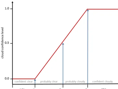
Figure 1. The linear approach of different confidence levels and
thresholds used for the cloud probability estimation from an obser-vation of variablex.
“AVHRR heritage” channels are used in APOLLO_NG. But, instead of binary yes/no information gained from “simple” threshold tests, the distance from the respective threshold is used as an estimate of the likelihood of cloud presence in the observation. A Bayesian probability update scheme then uses the cloud test probability (interpreted as confidence in observing a cloud with corresponding properties) for updat-ing the overall cloud probability. Figure 1 showcases how the distance from the threshold can be interpreted as a cloud probability. Binary threshold methods such as the traditional APOLLO scheme assume that, if an observed value is greater (lower) than a threshold, it is “definitely” cloudy or cloud free. Thus it assigns a cloud probability of either 0 or 1 to a specific cloud test without allowing for fractional probabili-ties. Consequently, the probabilistic extension is more flex-ible (allowing all probabilities between 0 and 1) and is also stricter in the mathematical interpretation. It propagates the probability in a clearly prescribed statistical way with equal weight for all cloud tests to the final cloud probability.
After having obtained an estimate of the cloud probability, the cloud affected pixels (over land) undergo a snow detec-tion test in the legacy of the Gesell et al. (1989) method. The minimum value of cloud probability for assigning an obser-vation to the cloud mask can be set according to the user’s needs. Consequently, the APOLLO_NG cloud detection can be tuned from clear sky confident (i.e., having low clear sky misclassification rate) to cloud confident (low cloud misclas-sification rate). This gives the user of the cloud detection scheme an increased cloud masking flexibility compared to the traditional APOLLO scheme.
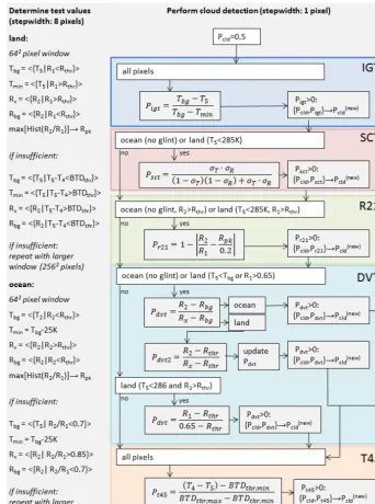
Figure 2 shows a detailed flowchart of the APOLLO_NG cloud detection. In contrast to the traditional APOLLO scheme the information of each individual cloud test feeds as Pcld into the outcome of the subsequent test. The
APOLLO_NG cloud detection scheme should be seen as a new algorithm rather than an update of the traditional APOLLO method. Nevertheless, both are based on the same physical principles of cloud detection.
2.2 Cloud probability, Bayesian probability
propagation and probabilistic information content Probabilistic cloud detection aims to evaluate the probability of cloud occurrence in a given observationx. Observations in this sense can be any observed property such as reflectance, brightness temperature, brightness temperature difference or reflectance ratio. For any observation an interval between values with a very high confidence for representing cloud-free background conditions (xbg)and values with a very high confidence for representing cloud observations (xcld)is de-fined. Figure 1 shows a schematic plot of the confidence in-terval concept.xbgandxcldcan be either predefined or they are determined from the satellite observations, for example by averaging over larger observation windows. The cloud probability for each cloud test then follows the linear met-ric
Ptest=
x−xbg
xcld−xbg
. (1)
It can be assumed that any observation can be approxi-mated by piecewise linearization around a traditional cloud mask thresholdxbinary. Thusxcldandxbgmust be selected to meet this assumption realistically, i.e., the interval [xbg,xcld] must not be too large for the character of given observation
xandxcld=xbgmust also be avoided.
A linear model for assessing the cloud likelihood around
xbinaryis chosen for the sake of convenience. The fact that it drops to zero atxbg already suggests that there may be bet-ter suited probability models like the Gaussian cumulative probability distribution function. Nevertheless, for the pur-pose of cloud detection the linear model is a good tradeoff between accuracy and computational convenience (and thus efficiency).
Bayesian statistics are used to propagate cloud likelihood information within different tests to aggregate the informa-tion gained from the different inputs.
Generally Bayes’ theorem states that the likelihood of one event can be calculated from the likelihood of all possible events and is traditionally used for updating probability in-formation for very different purposes (e.g., Rodgers, 1998; MacKay, 2003).
The version of Bayes’ theorem most often used in retrieval theory is
P (x|y)=P (y|x)·P (x)
P (y) , (2)
Figure 2. Flowchart of the APOLLO_NG cloud detection scheme.
the value of x andP (x|y)is the desired probability of the value forxgiven the evidenceP (y).
In the framework of cloud detection, one can assume that the evidence carrying signal is a binary symmetric channel, which means thatP (¬y)=1−P (y). This assumption be-comes important when updating the probability. In this case, furthermore using P (y)=P (y|x)P (x)+P (y|¬x)P (¬x), the updated probability ofx under the new evidence y be-comes (MacKay, 2004)
P (x|y)= P (x)·P (y|x)
(1−P (x))·(1−P (y|x))+P (x)·P (y|x), (3)
which is more convenient for the purpose of cloud detection than Eq. (2). The reason is that in Eq. (3) only two probability variables (P (x)andP (y|x)) are evaluated and the first guess about the prior evidenceP (y) is carried in the probability evaluation as the sum of the conditional probabilities forx
being true andxnot being true.
As the information in all above described cloud tests is complementary, Eq. (3) is used for probability propagation if the respective likelihoodP (y|x)given by a cloud test is larger than zero (i.e.,P (y|x) >0).
The overall cloud probability stems from the test proba-bilities of very different cloud characteristics. So, although strictly speaking the five tests do not assess the same prob-ability, their aggregation results in a good estimate of the probability that an observation really is cloud contaminated. In fact Pcld represents the probability that an observation shows a cloud having all five characteristics (cold top, bright reflectance, reflectance ratio about one, spatially inhomo-geneous and thin cloud, probably cirrus, at top). It is ob-tained by consecutive likelihood updates as described. Con-sequently, it can be used for cloud masking based on the de-sired confidence in either clear sky or cloudy pixel detection (see also discussion in Holzer-Popp et al., 2013).
In order to learn about the reliability of the cloud detec-tion, the cloud probabilities (those of the five different cloud tests outlined above) can be used as input to an assessment of Shannon’s information content Hinf (Shannon and Weaver, 1949; Kolmogorov, 1968; Rodgers, 2000; MacKay, 2004). Therefore the probabilities for cloud observation have to be interpreted as independent signals. Five signals about the cloud state build the basis for the information content:PIGT,
PSCT,PDVT,PR21,PT45 (detailed mathematical descriptions
follow in the sections below). In Shannon and Weaver (1949) the mathematical formulation of the information content re-quires that none of the probabilities equals 0 and also none equals one. Consequently, everyPx=0 would be set to 0.01
and everyPx=1 would be set to 0.99 for the purpose of
cal-culatingHinf.
The probabilistic information content concept of Kol-mogorov (1968) expands the view of Shannon and Weaver (1949) with respect to of Bayesian probability the-ory. Assuming that a priori information (i.e., information dependent of the aforementioned cloud tests) is zero, the in-formation content of the cloud detection algorithm emerges from the considerations of Kolmogorov (1968):
Hinf= − 5 X
j=1
Pj·log2 Pj. (4)
It is intuitive that the magnitude of Hinfis related to the information carried by the vector of cloud test probabilities. High information content signifies that the different proba-bilistic cloud tests agree quite well. This is a direct conse-quence of the definition of information content. Assuming that the probabilities would highly disagree, including one of the tests with rather low probability would not add any new information to the knowledge about the cloud. In the sense of Shannon and Weaver (1949) all information about the cloud contamination would already be known by hav-ing the information of one or two tests. On the other hand, when the tests have similar probabilities, each provides addi-tional information. Thus the resulting high information con-tent indicates that all cloud tests contribute to the knowledge about the cloud presence. The confidence then increases that the pixel is quite contaminated. Consequently, highHinf
re-lates to a more homogenous distribution of the probabilities. LowHinfindicates the significance of merely a single test for cloud detection. The more tests indicate cloudy (or cloud-free) conditions, the higher the confidence in the cloud de-tection. On the other hand, the original APOLLO was built in such a way that a single cloud test was able to classify an observation as cloudy. Consequently,Hinfprovides addi-tional information about the cloud detection. Together with
Pcld it thus may be used to tune the output towards a more “clear confident” cloud mask or a more “cloud confident” cloud mask, depending on the purpose of the product. 2.3 Probabilistic cloud detection tests
2.3.1 Infrared gross temperature (IGT)
Thick or cold-topped clouds can easily be detected in in-frared satellite imagery by their low brightness temperatures (e.g., Shenk and Curran, 1974; Saunders and Kriebel, 1988; Rosenfeld and Lensky, 1998; Frey et al., 2008). The infrared gross temperature test (IGT) makes use of the deviation be-tween observed cloudy brightness temperature in one of the split window channels (centered at 11 and 12 µm) and the background temperature representing the surface. In order to evaluate the brightness temperature distance from the most likely cloud-free brightness temperature, in APOLLO_NG a 65×65 (±32 pixels) pixels box around a given observations is evaluated.
Over ocean surfaces, a reflectance ratio for the channels 1 and 2 (centered at 0.6 and 0.9 µm, respectively), which is lower than 0.7, indicates mainly cloud-free conditions (Kriebel et al., 2003). Frey et al. (2008) use channel 2 re-flectance to identify cloud-free pixels with different confi-dence levels.
The aforementioned approach can be understood as clus-tering the data into confident cloud free and supposedly cloudy data and subsequent cluster-averaging. In order to speed up the procedure,TbgandTminare only calculated for 1 in 8 pixels and linearly interpolated in between (assum-ing steady and slowly vary(assum-ing background and cloud field temperature conditions). IGT cloud probabilityPIGTis then calculated for each pixel as
PIGT=
Tbg−T5
Tbg−Tmin
. (5)
If T5≤233.15 K and Tbg≤233.15 K (homogeneous freezing threshold, Pavolonis and Heidinger, 2004) it can be assumed that the target is a synoptic scale convective system, when also R1≥0.4. ThenPIGT is set to 0.95 without eval-uating Eq. (5) as in large scale synoptic systems it may be extremely difficult to find the appropriate background tem-peratureTbg. The value of 0.95 is an arbitrary choice in or-der to allow subsequent tests to include cloud information, which would not be possible as a consequence of Eq. (3) if
PIGTwould be set to 1 or even 0.99. 2.3.2 Spatial coherence test (SCT)
A spatial coherence test is used to examine regions with high variability in either reflectance or brightness tempera-ture (Saunders and Kriebel, 1988; Kriebel et al., 2003). In the APOLLO_NG algorithm the spatial coherence is evalu-ated consecutively in temperature and reflectance data during day. It starts with evaluating the 3×3 pixel standard deviation of the brightness temperature field (σT5)and of the channel 2
reflectance field (σR2). Coastal pixels are always
inhomoge-neous by definition and are thus discarded in the SCT like-lihood. Moreover, over land the SCT is only applied when
PIGT>0.
Applying Eq. (3) with likelihoods LT5=σT5/NPT5 and
LR2=σR2/NPR2the respective SCT cloud probabilityPSCT
is then evaluated as
PSCT=
LT5·LR2
1−LT5
·
1−LR2
+
LT5·LR2
. (6)
Cloud likelihood normalization parameters of NPT5=
1.0 K and NPR2 =0.2 are used for the standard deviations
of T5 and R2 (values adapted from Kriebel et al., 2003). Physically that means, the higher the standard deviation (the more variable the reflectance respective temperature field), the higher is the likelihood that the window is cloud af-fected and is mostly sensitive to broken or inhomogeneous cloud fields within the observation window. One should be aware that the standard deviation of the reflectance field is also subject to effects of variability of the bidirectional re-flectance distribution function (BRDF) of the surface over the 3×3 pixel box. It is assumed that in the presence of clouds these effects are minor compared to the impact of bright and inhomogeneous clouds given the small size of the sample.
2.3.3 Dynamic visible test (DVT)
Clouds can be identified as bright reflecting objects in satel-lite images (e.g., Shenk and Curran, 1974). Many different approaches have been identified to use reflectance thresh-olds for cloud discrimination (examples listed in e.g., Naka-jima and Kaufman, 1993, Frey et al., 2008, and Klüser et al., 2008). The dynamic visible test uses dynamic thresholds based on channel 2 (over ocean) or channel 1 (over land) re-flectance histograms for cloud identification. The approach is analogous to the IGT approach, but the scaling is performed with minimum cloudy and maximum clear sky reflectance for given confidence levels (Frey et al., 2008 as for IGT, see Sect. 2.3.1). Consequently, the DVT cloud likelihood is for-mulated as
PDVT=
R1,2−Rbg
Rbg−Rmax
, (7)
andRbgandRmaxare again evaluated for land and ocean sep-arately. Applying only Eq. (7) with the cluster-based back-ground and maximum reflectance values would result in high cloud probabilities over various land surfaces such as deserts or other bright surfaces. Thus the cloud probability is up-dated with Eq. (3) by using a priori background values for arid and non-arid land surfaces depending on the observed scenery. Following Frey et al. (2008) land surfaces are dis-tinguished between arid and non-arid (i.e., vegetated) by the minimum channel 1 reflectance in the running window. If the minimum reflectance falls below the clear sky value (high confidence) for non-arid land or the brightness temperature of the background is lower than 285 K, the filtering uses the non-arid values and the arid boundary thresholds are used otherwise. Any residual misinterpretation of desert surface properties for cloud probability is excluded by flagging all pixels that have non-negativePDVT, are warmer than 278 K, darker than 0.6 and have negative split window brightness temperature difference ofT4–T5(see e.g., Klüser and Schep-anski, 2009). Also very warm pixels (T2>290 K) for which the reflectance ratio test (see Sect. 2.3.4) yields zero prob-ability are discarded over land (a discussion on warm top clouds can also be found in Holzer-Popp et al., 2008). For these desert pixelsPDVTis set back to 0 in the case that the reflectance is lower than 0.65.
Over water bodies the DVT test is also sensitive to sunglint. Thus the DVT is not applied within the area po-tentially affected by sunglint, which can be determined from theoretical considerations (Saunders and Kriebel, 1988). 2.3.4 Shortwave reflectance ratio (R21)
reflectance ratios between 0.7 and 1.3 (Kriebel et al., 2003). The peak of the reflectance ratio histogram in the moving window is determined according to the description by Saun-ders and Kriebel (1988). The distance of the actual observa-tion from the peak is used to calculate PR21, if it is smaller
than 0.2 (that widens the original threshold of Saunders and Kriebel, 1988, in order to allow for a wider range of proba-bilities):
PR21=
(R2/R1)−(R2/R1)peak
0.2 . (8)
The reflectance ratio is used for cloud probability also over land (requiring thatT5<285 andT4–T5>0 in order to ex-clude warm desert surfaces). TheR21test is not executed in the sunglint area.
2.3.5 Brightness temperature difference (T45)
The test for thin clouds and cirrus is one of the most impor-tant for a couple of applications including aerosol retrieval (e.g., Holzer-Popp et al., 2013). Thin clouds can be detected by their differential influence on brightness temperatures at 11 and 12 µm (the so called split window channels) due to slopes in the complex refractive index of water and ice in that spectral region (e.g., Warren, 1984). Especially for cir-rus clouds the extinction efficiency is much lower at 11 than at 12 µm (Yang et al., 2005). The brightness temperature dif-ference (BTD) of AVHRR channels 4 and 5 has been used frequently for cirrus detection and visualization (e.g., Rosen-feld and Lenksy, 1998; Frey et al., 2008).
The thresholds for thin cloud detection vary with observed channel 4 brightness temperature as well as with the cosine of the viewing zenith angle2v(Saunders and Kriebel, 1988). In order to determine the thin cloud probability from theT45 test the BTD thresholds of Saunders and Kriebel (1988) are evaluated for a range of conditions enveloping the actual con-ditions (namely,T4and cos(2v)). From these envelope con-ditions the minimum and maximum BTD (named BTDmin and BTDmax, respectively) are determined and the thin cloud probability is evaluated as for the other tests:
PT45=
BTD−BTDmin BTDmax−BTDmin
. (9)
2.3.6 Additional nighttime probability estimates (T43 andT35)
At night, the channels 1 and 2 cannot be exploited for cloud detection, as no reflected sunlight is available. Neverthe-less, the channel 3 of AVHRR is available at night for all three AVHRR versions. For the AVHRR/1 and AVHRR/2 in-struments, the channel 3 is permanently centered at 3.7 µm, while for AVHRR/3 the channel 3 mode is switched between 1.6 µm at day and 3.7 µm at night. Instruments such as SE-VIRI, AATSR or VIIRS operate both, 1.6 and 3.7 (or 3.9) µm channels permanently. Consequently, for these instruments
the 3.7 (3.9) µm brightness temperature is used as additional input at night. Following Kriebel et al. (2003) the bright-ness temperature differences between channel 4 and channel 3 and between channel 3 and channel 5 are exploited during night (T43 respectiveT35). The lower and upper boundaries (BTDminrespective BTDmaxin Eq. 9) of the probability esti-mation interval are 0.5 and 1.5 K in the first and 3 and 5 K in the latter (1 K respective 2 K confidence interval around the thresholds used in Kriebel et al., 2003).
3 Snow discrimination
The a posteriori snow detection (i.e., detection of falsely identified clouds in the case of snow cover) follows the same probabilistic approach as the cloud detection scheme. That is, the binary thresholds in Kriebel et al. (2003) and Gesell (1989) are expanded by the methodology explained above in order to yield a snow contamination probability. The snow discrimination is only applied over land and for ob-servations with 258 K≤T5≤278 K. Also2s<85◦,PT45=
0 and PDVT>0 are necessary prerequisites for successful snow detection. That means, the pixel must be illuminated by sun, must not be cirrus contaminated and the dynamic visible reflectance test must indicate cloud. Then the snow detection is performed applying Eq. (7) to the channel 3 reflectanceR3. The boundary thresholds are Rbg=0.1 and
Rmax=0.03 (which only becomes positive whenR3< Rbg) in the case of channel 3 being centered at 3.7 µm. Otherwise, i.e., channel 3 center wavelength of 1.6 µm,Rbg=0.15 and
Rmax=0.06. The snow probability is updated once again by using the reflectance ratio between channels 1 and 3 with the confidence interval boundariesRbg=20,Rmax=15 for the 3.7 µm channel andRbg=6.67,Rmax=5 for the 1.6 µm channel.
4 Cloud property retrieval
4.1 Optical depth and effective radius
Figure 3. Reflectance of liquid water (left) and ice (right) clouds at the absorbing versus the non-absorbing channel for the absorbing channel
being centered at 1.6 µm (top) and 3.7 µm (bottom). Cloud reflectance is simulated with the two-stream scheme of Coakley and Chylek (1975) for a sun zenith angle or 10◦and for various optical depths and effective radii (see text for details).
As inherited from the original APOLLO it is assumed that the solution of the radiative transfer problem used in tradi-tional schemes does a reasonably good job for AVHRR. In fact the signal-to-noise ratio as well as the broad spectral re-sponse functions of the solar bands of AVHRR (together with the calibration) suggest that using a two-stream approxima-tion will provide reasonably good results. In APOLLO_NG the two-stream solution of the radiative transfer problem as described in Coakley and Chylek (1975) is used for the non-absorbing and the non-absorbing channel. This scheme is iden-tical to the scheme used for the original APOLLO cloud property retrieval (Kriebel et al., 1989) and thus truly com-plies with the APOLLO legacy. The surface is assumed to be Lambertian with the albedo estimated from the cloud-free surroundings as described in Sect. 2.3.3.
The two-stream approach used in APOLLO_NG offers the potential to calculate reflectance online at reasonably high performance. This gives the advantage that the method be-comes independent of sensor-specific radiance lookup tables and tuning factors (as long as the channel specific cloud single scattering albedo and asymmetry parameter are pro-vided, both essential inputs to the two-stream approxima-tion) – of course at the price of reduced accuracy (see dis-cussion in Coakley and Chylek, 1975). The second advan-tage is that the calculations can be performed online for a range of optical depths and effective radii, so that the
proba-bilistic potential can be fully exploited. It nevertheless has to be made absolutely clear that the two-stream approach buys the mathematical simplicity at the price of losing ac-curacy in the results. That becomes of larger importance for sensors with better calibrated solar channels having narrow filter functions. Consequently, the results obtained by using the two-stream approach as outlined below should be seen as rough estimates in the case of instruments such as SEVIRI, AATSR or VIIRS. They are used here for the sake of con-sistency with the AVHRR methodology and not because we think they will offer high precision. Moreover, as the tradi-tional APOLLO scheme has been shown to be useful for ex-ample in solar irradiance calculations (Oumbe et al., 2013) it is envisaged to keep the physics of the traditional APOLLO scheme. The new implementation in APOLLO_NG com-pared to APOLLO thus mainly consists of incorporating the effective radius retrieval and the probabilistic approach also yielding uncertainties for the retrieved parameters.
and black curves would correspond to the possibility of re-trieving optical depth and effective radius independently, as is more or less the case for very high optical depths. At lower optical depth the sensitivity to effective radius changes de-creases, and as a result the uncertainty in retrieved effective radius will become much higher.
For the 3.7 µm channel of AVHRR under daylight condi-tions it is essential to correct for the thermal emission in order to calculate the reflected part of the signal. Figure 3 shows that getting an improper reflectance in the absorbing chan-nel will cause large errors in the retrieved effective radius, but also in the optical depth. The method of Kaufman and Nakajima (1993) also takes into account above-cloud water vapor absorption for calculation of 3.7 µm reflectance and is applied within APOLLO_NG.
The simultaneous retrieval of cloud optical depth and ef-fective radius (Nakajima and King, 1990) is performed con-secutively for each observation for potential liquid water and ice phase clouds. The approach is to calculate optical depths with the equations of Coakley and Chylek (1975) and Stephens et al. (1984) from a set of 10 different reflectance values R1,sim in the red (non-absorbing) channel ranging from 0.05 to 0.95. For each of these 10 values forR1,sim the distance to the observationR1is determined. The weighting factor for each R1,sim is then calculated assuming a Gaus-sian distribution around the observation R1with a standard deviation of 10 %. A first guess optical depth is determined by weighting the optical depth values associated with each reflectance value by the thus determined Gaussian weighting factor. Having obtained first guess optical depth, the same procedure is repeated with a set of 10 different effective radii for the reflectance in the absorbing channel, yieldingR3,sim. The Gaussian distribution of the thus simulated reflectance around the observationR3provides the weighting factors for the effective radius. The resulting effective radius (evaluated for assumed liquid water and ice clouds separately) is again calculated by weighting the input values with the weighting factors. Moreover the first guess optical depth is once again corrected for the influence of the effective radius on the non-absorbing reflectance (through the phase function and thus the backscattered fraction).
Starting values for the effective radius are 2 µm through 20 µm in 2 µm steps for liquid water clouds and 10 µm through 55 µm in 5 µm steps for ice clouds. Necessary sin-gle scattering albedo and asymmetry parameter (see Coakley and Cox, 1975; Stephens et al., 1984) are determined with Mie calculations for liquid water clouds. For the sake of con-venience and as the results for different effective radius val-ues are combined in the probabilistic scheme, we performed the Mie simulations for mono-disperse liquid-water clouds. For ice clouds the optical properties of Baum et al. (2014) are used.
Within the APOLLO_NG scheme not only the mean val-ues for optical depth and effective radius are calculated, but also the standard deviation of the thus-obtained probability
distributions. This methodology easily allows for estimating the uncertainty of the retrieved quantity. Consequently, each retrieval is accompanied by an uncertainty estimate, which is a prerequisite e.g., for data assimilation in numerical models. 4.2 Cloud top phase, cloud top temperature and cloud
water path
During the previous step two values for cloud optical depth and effective radius have been obtained: one for purely liquid phase clouds and one for ice clouds. Cloud phase discrimi-nation yields the final value for optical depth and effective radius through representative weighting following the prob-abilistic approach. Therefore the Gaussian distributions for the weighting factors of the simulated channel 3 reflectances (depending on the selected effective radii) are used for evalu-ating the likelihood of liquid water respective ice clouds. As the absorbing channel is sensitive to the cloud phase as well as to the effective radius, theR3,simforward simulations are also well suited for cloud phase assessment. It is assumed that the sum over all distance weighting factors is smaller for the cloud phase better representing the observed cloud. Con-sequently, the first guess of the liquid phase fraction is simply calculated as
LPF1=
P
jφj(liquid) P
jφj(liquid)+Pjφj(ice)
. (10)
φjdenotes the weighting factor for thejth effective radius
value for liquid water or ice clouds respectively. If no cirrus cloud is detected, i.e., if the topmost cloud layer is assumed to be opaque, the liquid phase fraction is once more updated with the likelihood of glaciated cloud droplet expressed as a function of temperature. Therefore it is assumed that be-low the homogeneous freezing temperature of 233.15 K all droplets at cloud top are frozen and that above the pure wa-ter freezing point of 273.15 K all cloud droplets are liquid (Pavolonis and Heidinger, 2004). Thus applying Eq. (3) with these boundary thresholds yields an updated liquid phase fraction (LPF) of
LPF
=
LPF1·
T5−233.16 K
40 K
(1−LPF1)·
1−T5−233.16 K
40 K
+LPF1· T
5−233.16 K
40 K
(11) for any observation with 233.15 K≤T5≤273.15 K. More-over for T5>273.15 K, LPF=1 and for T5<233.15 K, LPF=0. Cloud optical depth and effective radius are then finally determined by weighting the results for liquid clouds by LPF and those for ice clouds by (1−LPF).
between cloudy and clear radiance (IcldandIclr, respectively) and the channel 5 radianceI5. The corresponding equation (e.g., Guignard et al., 2012)
1−exp(−τ )= I2−Iclr
Icld−Iclr
(12) can easily be solved forIcld. It directly yields cloud top tem-perature through inversion of the temtem-perature–radiance re-lationship. Iclr is approximated by the background temper-ature value Tbg as determined for the IGT cloud probabil-ity. Infrared optical depth τir is different from visible opti-cal depth τvis for non-opaque clouds (e.g., Comstock et al., 2007; Baum et al., 2014). Here the approximation of Chang and Li (2005) is used, which relatesτirtoτvisby
τir=
τvis
LPF·2.13+(1−LPF)·2.56. (13) Cloud water path can be expressed as a function of optical depth and effective radius as well as extinction efficiencyQe. For spherical liquid phase cloud dropletsQe→2, while for ice clouds the extinction efficiency is determined by effective radius (and the crystal shape) and thus is determined from the weighting factors of the effective radius from the optical properties database. Liquid phase and ice phase extinction efficiencies are weighted according to the liquid phase frac-tion (the same is done for densityρ). Then the cloud water path is calculated as
CWP=4·ρ·τvis·reff 3·Qe
. (14)
Besides the liquid phase fraction (or ice phase fraction IPF=1−LPF) also a cloud top phase identifier is derived in order to facilitate the interpretation and application of APOLLO_NG results. It is widely controlled by LPF and CTT as well asPT45.
As a starting point all observations having CTT > 273.15 K or LPF > 0.75 are identified as liquid water clouds. Correspondingly, all clouds having CTT≤273.15 K and LPF < 0.05 are initially set to opaque ice clouds. If CTT≤ 273.15 K and 0.05≤LPF≤0.75 the clouds are classified as supercooled liquid/mixed phase. In the case thatPT45
indi-cates thin cloud, presence of cirrus is assumed ifT5> 233.15 (i.e., the cloud is not opaque with cold-top such as deep con-vective clouds) and CTT < 253.15 K (i.e., the cloud top is rea-sonably cold for cirrus). Given cirrus has been identified but the optical depth is larger than 2 and more than one test indi-cates the presence of clouds (i.e.,Hinf> 0) it is assumed that more than one cloud layer is present and the overlap flag is set.
In the cloud detection scheme the cloud fraction of each pixel is approximated by the cloud probability as a start-ing point. Thus observations withPcld< 95 % are assumed to be partially cloudy. That follows the legacy of the original APOLLO scheme. During the cloud property retrieval the
fractional cloud cover is estimated from the average of the first guess cloud fraction of a surrounding 3×3 pixel box. Hence it is assumed that near cloud edges the information carried by neighboring pixels translates into subpixel cloudi-ness (see e.g., Koren et al., 2008; Hirsch et al., 2014).
5 Example results from AVHRR
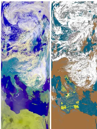
Figure 4 depicts the RGB composite and cloud mask in the traditional APOLLO quicklook style for an overpass of NOAA-18 over Europe in HRPT (High Resolution Pic-ture Transmission) projection with 1.1 km spatial resolution at nadir received at the receiving station of the German Aerospace Center (DLR) at Oberpfaffenhofen, South Ger-many, for 15 July 2008. In the cloud mask image fully cloudy pixels are white, partially cloudy pixels grey, sunglint is yel-low, cloud-free water is blue and cloud-free land brown (see Kriebel et al., 2003). Both images have been produced with APOLLO_NG strictly following the tradition of APOLLO. The cloud mask derived from APOLLO_NG and depicted in Fig. 4 includes all pixels with cloud probability larger than 25 %.
Figure 5 shows an example of APOLLO_NG cloud prob-abilityPcld and the corresponding cloud detection informa-tion content Hinf for the AVHRR scene on 15 July 2008 in isotropic Mercator projection with 1/30◦grid resolution. Clouds have been detected over wide parts of central and northern Europe with high confidence. The information con-tent on the other hand shows that not in all cases with high cloud probability all cloud tests agree as the variability in
Hinf is much higher than the variability in Pcld. Given the dependences of the different cloud tests, it is not surpris-ing that the information content is highest for cumulus and stratocumulus cloud fields with high spatial variability (e.g., northwest of Great Britain and over central Europe) and not that high for the cyclonic deep convection in the vicinity of Iceland. In the latter case ice-topped cold clouds with rather high spatial homogeneity prevail, reducing the suitability of the SCT,R21andT45tests. Comparing Fig. 4 (the cloud mask derived fromPcld>25 %) and Fig. 5 shows that there are re-gions where cloud probability is low (for example < 25 %) and it is not obvious from visual inspection of the RGB im-age that these are indeed cloud contaminated. Such regions are for example found in central France, over North Africa and over the Mediterranean Sea. Consequently, an adjust-ment of the clear sky threshold forPcld to 25 % results in a larger number of clear sky pixels compared to what would be flagged with a threshold ofPcld>0 %. Such a possibil-ity of adjustment is especially important for the purpose of aerosol retrieval (Holzer-Popp et al., 2013) and solar irradi-ance estimation.
Figure 4. RGB composite and cloud mask in the traditional APOLLO quicklook style (Kriebel et al., 2003; see also text for color description)
from AVHRR on NOAA-18 for 15 July 2008 in orbit projection.
the resulting cloud mask in this example is a bit more on the clear conservative side than on the cloud conservative side. Recent analysis of SEVIRI cloud detection suggests that the cloud mask of the traditional APOLLO scheme is best represented by setting a cloud probability of 40 % (not shown). That value may change with sensor, as the traditional APOLLO versions slightly vary with sensor. It is another in-dicator that the 25 % minimumPcldthreshold used for gener-ating the cloud mask in Fig. 4 and subsequently for deriving the cloud products (Fig. 6) is rather clear conservative.
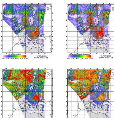
Figure 6 shows the resulting cloud optical depth and ef-fective radius for the same AVHRR scene together with their
Figure 5. Cloud probability (left) and cloud detection information content (right) from AVHRR on NOAA-18 for 15 July 2008.
Figure 6. Cloud optical depth (top row) and effective radius (bottom row) retrieval results (left) and associated uncertainties (right) for the
same data as in Fig. 4.
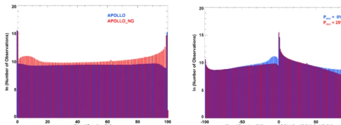
Figure 7. Left – cloud fraction histograms of APOLLO (red) and APOLLO_NG (blue) for the central overpass of NOAA-19 on 15 July 2013.
Right – histograms of the cloud fraction difference between APOLLO and APOLLO_NG for all cloud probability values (blue) and with all observations having cloud probability smaller than 25 % set to cloud free (red).
uncertainties are observed for high effective radii, i.e., for ice clouds, or in cases of low cloud optical depth.
In Figure 7 histograms of cloud fraction for one AVHRR overpass over Europe (15 July 2013, daytime) are presented for APOLLO_NG as well as for the original APOLLO scheme. It can be seen that APOLLO tends to detect much more either fully cloudy or entirely cloud-free pixels (the population of the histogram bins are depicted as the nat-ural logarithm of the numbers of observations), whereas APOLLO_NG has higher shares of cloud fractions between 1 and 99 %. The histograms of the cloud fraction differ-ences between APOLLO and APOLLO_NG are as well presented. Here the blue bars indicate the difference dis-tribution when all pixels are taken into account regard-less of the APOLLO_NG cloud probability, and also when APOLLO_NG pixels with cloud probabilities smaller than 25 % are set to cloud free (red bars). It is evident that in the latter case the amount of rather large positive differ-ences (i.e., APOLLO has much higher cloud fraction than APOLLO_NG) decreases. The two histograms exemplarily show the potential benefit of changing the minimum cloud probability for cloud detection. Although in Fig. 7 only one springtime overpass over Europe covering a wide range of complex cloud conditions is analyzed, histograms from other overpasses in all four seasons show very similar results. This comparison should not be seen as a rigorous validation, but it gives a first indication about the performance of the APOLLO_NG cloud detection. Referring to the evaluation of the traditional APOLLO scheme, 70 % of cloud cover re-trievals showed agreement within±1/8 cloud amount when compared to SYNOP observations (Kriebel et al., 2003). The comparison of APOLLO and APOLLO_NG shows agree-ment of 78.4 % (all observations) to 79.3 % (minimum cloud probability of 25 %) within±1/8 (cloud fraction±12.5 %).
6 Discussion
The examples presented above showcase the possibility of using the original APOLLO cloud detection metrics and physical parameterizations in a probabilistic manner. Such an approach increases the information gained from AVHRR observations. With the probabilistic approach the desired de-gree of conservativeness in the cloud detection can be tuned from clear confident to cloud confident. This is achieved by selecting an appropriate minimum cloud probability for iden-tifying cloud contaminated pixels. In applications of cloud property remote sensing the minimum probability will be set rather high. Contrastingly in cloud masking applications for clear sky remote sensing purposes, such as for example aerosol retrieval, the minimum probability will be selected rather low. Each evaluation of the cloud mask must thus take into account the corresponding purpose as well as the selec-tion of minimum probability. In Fig. 4 it has been shown that cloud probability alone will result in a cloud mask which can be adapted to the purpose of usage (see Fig. 7), but the quality of the cloud detection can furthermore been assessed by the interpretation of the Shannon information contentHinf pro-vided along withPcld. The more cloud tests detect potential cloud contamination and thus the higherHinf, the more con-fidence one can have in the retrieved cloud probability (even if it is a low probability).
is also used in APOLLO_NG, extended by the formulation of the two-stream equations for absorbing channels (Coak-ley and Chylek, 1975). We are fully aware that using a two-stream approximation will reduce the precision of the re-flectance simulations. Nevertheless, performing the simula-tions online is seen to be advantageous over the loss of preci-sion for the purpose of APOLLO_NG. Moreover, simulating the 3.7 µm reflectance would require very good knowledge about the cloud top temperature a priori. This knowledge typically is not available. Consequently, the errors brought about by the estimation of the thermally emitted part of the 3.7 µm band radiance would again result in large errors which would remove all advantages from the precise radiative trans-fer modeling. This would not be a large problem for sen-sors such as SEVIRI or VIIRS which also have absorbing channels at 1.6 or 2.2 µm. For the AVHRR/1 and AVHRR/2 with the 3.7 µm channel the errors introduced by the use of the two-stream approximation are expected to not be larger than those of the other estimations and assumptions. Espe-cially the conversion from thermal-corrected radiance to re-flectance includes the assumption of Lambertian reflection and potentially introduces additional errors. Also, given the rather broad channel response functions of the AVHRR in-struments, the uncertainties of the two-stream approxima-tion might be acceptable compared to their influence for instruments with finer resolution. In contrast to the tradi-tional APOLLO scheme the APOLLO_NG implementation rigorously follows a modular programming approach. Con-sequently, the two-stream scheme could easily be replaced with a more precise forward model. The value of this will be explored for applications of APOLLO_NG to more modern sensors than AVHRR.
Online simulations together with the probabilistic ap-proach of retrieving cloud properties have the great ad-vantage that uncertainty assessment is an intrinsic by-product of each retrieved variable. Consequently, the un-certainty of each observation (i.e., pixel) is estimated from the observations itself. Figure 6 clearly shows the value of such a method. Depending on the purpose of the use of APOLLO_NG results these uncertainties also can be used to confine the applications to observations with high confi-dence only. This will be especially useful in the application of APOLLO_NG in high resolution case studies (e.g., Klüser et al., 2008) or in the field of aerosol-cloud-interaction re-search (Klüser et al., 2008; Klüser and Holzer-Popp, 2010).
In this study the methodology of the probabilistic APOLLO_NG scheme has been outlined. The specific cloud detection tests have been motivated from well-known phys-ical principles and standard methodologies of cloud re-mote sensing. Cloud detection and cloud property evalu-ation is currently performed for APOLLO_NG by differ-ent means and for a range of sensors. Cloud detection will first be cross compared with cloud detection results of the original APOLLO scheme, which has already been evaluated with SYNOP data for AVHRR and for Europe
(Kriebel et al., 2003; Meerkötter et al., 2004). This cross-comparison has already been started and will be described in a subsequent study. Moreover APOLLO_NG will be run with MODIS (Moderate Resolution Imaging Spectrora-diometer) and VIIRS observations and will be compared with independent cloud mask results from the MODIS/VIIRS cloud detection (which exploit more channels of these in-struments than APOLLO_NG does, see for example Frey et al., 2008). In order to evaluate the cloud property re-trievals, the APOLLO_NG results will also be compared to MODIS/VIIRS cloud retrievals. Using external data as a reference also facilitates sensitivity studies, especially in terms of relationships between minimum cloud probability and false alarm rate and cloud detection rate. Moreover the availability of a wide range of channels including those cen-tered at 1.3, 1.6, 2.2 and 3.7 µm provides the possibility to assess the sensitivity of the retrieved cloud properties to the selection of the absorbing channel. Consequently, the exter-nal uncertainties and potential biases for sensors having only one of the useful channels (like AVHRR) can be examined.
7 Summary and outlook
Based on the legacy and the physical principles of the well-known cloud retrieval scheme APOLLO a new scheme called APOLLO_NextGeneration has been developed. By build-ing on the classical principles for cloud detection and cloud property retrieval, these have been implemented in a prob-abilistic way. This study explained the physical and math-ematical principles and approaches used in the formula-tion of the APOLLO_NG scheme and shows example re-sults with AVHRR. One of the major achievements of the APOLLO_NG scheme is to harmonize the legacy of the APOLLO method for all satellite sensors maintaining the so-called AVHRR heritage channels. So far each sensor had its own APOLLO adaptation (see Kriebel et al., 2003; Holzer-Popp et al., 2008; Klüser and Holzer-Holzer-Popp, 2010). Conse-quently, a harmonization effort was strongly required for fu-ture applications and extended evaluation of cloud products and derived information. As the APOLLO_NG makes use of a probabilistic approach to cloud detection, it thus addresses the need of variable cloud detection conservativeness in a broad range of applications (e.g., Holzer-Popp et al., 2013). Traceability of the origins of the reported cloud probability as well as flexible cloud detection thresholds together with a propagation of information allows for a more useful descrip-tion of the observed condidescrip-tions (Fig. 7). New addidescrip-tional inter-pretations of the cloud detection results such as the Shannon information content for cloud detection moreover feed into the potential to define cloud masks addressing the purpose of the application.
APOLLO. This comparison has been done for cloud frac-tion and for one overpass over Europe in this study. Com-paring the resulting numbers with other overpasses in other seasons indicated that these remain fairly constant. Never-theless, a more rigorous validation of the cloud detection and cloud property retrieval is necessary and will be covered in full detail in a subsequent study.
Introducing the retrieval of cloud droplet (and ice crys-tal) effective radius into the scheme makes APOLLO_NG also a suitable candidate for aerosol-cloud-interactions re-search (see Klüser and Holzer-Popp, 2010). APOLLO_NG facilitates the possibility to continue and expand the use of APOLLO in a wide range of applications (e.g., Gesell, 1989; Meerkötter et al., 2004; Holzer-Popp et al., 2008; Klüser and Holzer-Popp, 2010; Qu et al., 2012). All of these applications require a well-understood error characterization as well as clearly documented sensitivities of the APOLLO_NG cloud products. Consequently, a subsequent APOLLO_NG evalu-ation study will use MODIS and VIIRS data to derive the sensitivity to absorbing channel selection between 1.6 and 3.7 µm. Moreover, it will cross-examine the cloud property results with the MODIS/VIIRS cloud products at given sen-sor resolution and geometry.
Acknowledgements. We thank three anonymous reviewers for their
constructive comments and valuable suggestions, which helped to improve the manuscript. The development of the APOLLO_NG method was part of the DLR project TIMELINE.
The article processing charges for this open-access publication were covered by a Research
Centre of the Helmholtz Association.
Edited by: A. Sayer
References
Baum, B. A., Yang, P., Heymsfield, A. J., Bansemer, A., Cole, B. H., Merrelli, A., Schmitt, C., and Wang, C.: Ice cloud single-scattering property models with the full phase matrix at wave-lengths from 0.2 to 100 µm, J. Quant. Spectrosc. Ra., 146, 123– 139, doi:10.1016/j.jqsrt.2014.02.029, 2014.
Chang, F.-L. and Li, Z.: A new method for detection of cirrus over-lapping water clouds and determination of their optical proper-ties, J. Atmos. Sci., 62, 3993–4009, 2005.
Coakley, J. A. and Chylek, P.: The two-stream approximation in ra-diative transfer: including the angle of incident radiation, J. At-mos. Sci., 32, 409–418, 1975.
Comstock, J. M., d’Entremont, R., DeSlover, D., Mace, G. G., Matrosov, S. Y., McFarlane, S. A., Minnis, P., Mitchell, D., Sassen, K., Shupe, M. D., Turner, D. D., and Wang, Z.: An in-tercomparison of microphysical retrieval algorithms for upper-tropospheric ice clouds, B. Am. Meteorol. Soc., 88, 191–204, 2007.
Frey, R. A., Ackerman, S. A., Liu, Y., Strabala, K. I., Zhang, H., Key, J. R., and Wang, X.: Cloud detection with
MODIS. Part I: Improvements in the MODIS cloud mask for collection 5, J. Atmos. Ocean. Tech., 25, 1057–1072, doi:10.1175/2008JTECHA1052.1, 2008.
Gesell, G.: An algorithm for snow and ice detection using AVHRR data an extension to the APOLLO software package, Int. J. Re-mote Sens., 10, 897–905, 1989.
Guignard, A., Stubenrauch, C. J., Baran, A. J., and Armante, R.: Bulk microphysical properties of semi-transparent cirrus from AIRS: a six year global climatology and statistical analy-sis in synergy with geometrical profiling data from CloudSat-CALIPSO, Atmos. Chem. Phys., 12, 503–525, doi:10.5194/acp-12-503-2012, 2012.
Hirsch, E., Koren, I., Levin, Z., Altaratz, O., and Agassi, E.: On transition-zone water clouds, Atmos. Chem. Phys., 14, 9001– 9012, doi:10.5194/acp-14-9001-2014, 2014.
Holzer-Popp, T., Schroedter-Homscheidt, M., Breitkreuz, H., Mar-tynenko, D., and Klüser, L.: Improvements of synergetic aerosol retrieval for ENVISAT, Atmos. Chem. Phys., 8, 7651–7672, doi:10.5194/acp-8-7651-2008, 2008.
Holzer-Popp, T., de Leeuw, G., Griesfeller, J., Martynenko, D., Klüser, L., Bevan, S., Davies, W., Ducos, F., Deuzé, J. L., Graigner, R. G., Heckel, A., von Hoyningen-Hüne, W., Kolmo-nen, P., Litvinov, P., North, P., Poulsen, C. A., Ramon, D., Sid-dans, R., Sogacheva, L., Tanre, D., Thomas, G. E., Vountas, M., Descloitres, J., Griesfeller, J., Kinne, S., Schulz, M., and Pin-nock, S.: Aerosol retrieval experiments in the ESA Aerosol_cci project, Atmos. Meas. Tech., 6, 1919–1957, doi:10.5194/amt-6-1919-2013, 2013.
Kaufman, Y. J. and Nakajima, T.: Effect of Amazon smoke on cloud microphysics and albedo – analysis from satellite imagery, J. Appl. Meteorol., 32, 729–744, 1993.
Klüser, L. and Holzer-Popp, T.: Relationships between mineral dust and cloud properties in the West African Sahel, Atmos. Chem. Phys., 10, 6901–6915, doi:10.5194/acp-10-6901-2010, 2010. Klüser, L. and Schepanski, K.: Remote sensing of mineral dust
over land with MSG infrared channels: A new Bitemporal Mineral Dust Index, Remote Sens. Environ., 113, 1853–1867, doi:10.1016/j.rse.2009.04.012, 2009.
Klüser, L., Rosenfeld, D., Macke, A., and Holzer-Popp, T.: Obser-vations of shallow convective clouds generated by solar heat-ing of dark smoke plumes, Atmos. Chem. Phys., 8, 2833–2840, doi:10.5194/acp-8-2833-2008, 2008.
Kolmogorov, A. N.: Logical basis for information theory and prob-ability theory, IEEE T. Inform. Theory, 14, 662–664, 1968. Koren, I., Oreopoulos, L., Feingold, G., Remer, L. A., and
Al-taratz, O.: How small is a small cloud?, Atmos. Chem. Phys., 8, 3855–3864, doi:10.5194/acp-8-3855-2008, 2008.
Kriebel, K. T., Saunders, R. W., and Gesell, G.: Optical properties of clouds derived from fully cloudy AVHRR pixels, Beitr. Phys. Atmosph., 62, 165–171, 1989.
Kriebel, K. T., Gesell, G., Kästner, M., and Mannstein, H.: The cloud analysis tool APOLLO: improvements and validations, Int. J. Remote Sens., 24, 2389–2408, 2003.
MacKay, D. J. C.: Information Theory, Inference and Learning Al-gorithms, Cambridge University Press, Cambridge, UK, 2004. Merchant, C. J., Harris, A. R., Maturi, E., and Maccallum, S.:
Meerkötter, R., König, C., Bissoli, P., Gesell, G., and Mannstein, H.: A 14-year European Cloud Climatology from NOAA/AVHRR data in comparison to surface observations, Geophys. Res. Lett., 31, L15103, doi:10.1029/2004GL020098, 2004.
Nakajima, T. and King, M. D.: Determination of the optical thick-ness and effective particle radius of clouds from reflected so-lar radiation measurements – Part I: Theory, J. Atmos. Sci., 47, 1878–1893, 1990.
Oumbe, A., Blanc, P., Ranchin, T., Schroedter-Homscheidt, M., and Wald, L.: A new method for estimating solar energy resource, in: Proceedings of the ISRSE 33, Stresa, Italy, 4–9 May 2009, Joint Research Center, Ispra, Italy, USBKey, paper 773, 2009. Pavolonis, M. J. and Heidinger, A. K.: Daytime cloud overlap
detec-tion from AVHRR and VIIRS, J. Appl. Meteorol., 43, 762–778, 2004.
Qu, Z., Oumbe, A., Blanc, P., Lefevre, M., Wald, L., Schroedter-Homscheidt, M., Gesell, G., and Klüser, L.: Assessment of Heliosat-4 surface solar irradiance derived on the basis of SEVIRI-APOLLO cloud products, Proceedings of the 2012 EU-METSAT Meteorological Satellite Conference, Sopot, Poland, 3–7 September 2012, EUMETSAT P. 61, s2–06, 2012.
Rosenfeld, D. and Lensky, I. M.: Satellite-based insights into pre-cipitation formation processes in continental and maritime con-vective clouds, B. Am. Meteorol. Soc., 79, 2457–2476, 1998. Rodgers, C.D.: Information content and optimization of high
spec-tral resolution remote measurements, Adv. Space Res., 21, 361-367, 1998.
Rodgers, C. D.: Inverse methods for atmospheric sounding, theory and practice, in: Series on Atmospheric, Oceanic and Planetary Physics, vol. 2, World Scientific Publishing, Singapore, 2000. Saunders, R. W. and Kriebel, K. T.: An improved method for
de-tecting clear sky and cloudy radiances from AVHRR data, Int. J. Remote Sens., 9, 123–150, 1988.
Shannon, C. E. and Weaver, W.: The Mathematical Theory of Com-munication, University of Illinois Press, 1949.
Shenk, W. E. and Curran, R. J.: The detection of dust storms over land and water with satellite visible and infrared measurements, Mon. Weather Rev., 102, 830–837, 1974.
Stephens, G. L.: Radiation profiles in extended water clouds. II: Pa-rameterization schemes, J. Atmos. Sci., 35, 2123–2132, 1978. Stephens, G. L., Ackerman, S., and Smith, E. A.: A shortwave
pa-rameterization revised to improve cloud absorption, J. Atmos. Sci., 41, 687–690, 1984.
Yang, P., Wei, H., Huang, H.-L., Baum, B. A., Hu, Y. X., Kat-tawar, G. W., Mishchenko, M. I., and Fu, Q.: Scattering and absorption property database for nonspherical ice particles in the near- through far-infrared spectral region, Appl. Optics, 44, 5512–5523, 2005.