www.clim-past.net/13/379/2017/ doi:10.5194/cp-13-379-2017
© Author(s) 2017. CC Attribution 3.0 License.
Development and evaluation of a system of proxy data
assimilation for paleoclimate reconstruction
Atsushi Okazaki1and Kei Yoshimura2
1RIKEN Advanced Institute for Computational Science, Kobe, Japan 2Institute of Industrial Science, The University of Tokyo, Tokyo, Japan
Correspondence to:Atsushi Okazaki ([email protected])
Received: 21 November 2016 – Discussion started: 22 November 2016
Revised: 26 February 2017 – Accepted: 28 March 2017 – Published: 20 April 2017
Abstract.Data assimilation (DA) has been successfully ap-plied in the field of paleoclimatology to reconstruct past cli-mate. However, data reconstructed from proxies have been assimilated, as opposed to the actual proxy values. This pre-vented full utilization of the information recorded in the proxies.
This study examined the feasibility of proxy DA for pale-oclimate reconstruction. Isotopic proxies (δ18O in ice cores, corals, and tree-ring cellulose) were assimilated into mod-els: an isotope-enabled general circulation model (GCM) and forward proxy models, using offline data assimilation.
First, we examined the feasibility using an observation system simulation experiment (OSSE). The analysis showed a significant improvement compared with the first guess in the reproducibility of isotope ratios in the proxies, as well as the temperature and precipitation fields, when only the iso-topic information was assimilated. The reconstruction skill for temperature and precipitation was especially high at low latitudes. This is due to the fact that isotopic proxies are strongly influenced by temperature and/or precipitation at low latitudes, which, in turn, are modulated by the El Niño– Southern Oscillation (ENSO) on interannual timescales.
Subsequently, the proxy DA was conducted with real proxy data. The reconstruction skill was decreased compared to the OSSE. In particular, the decrease was significant over the Indian Ocean, eastern Pacific, and the Atlantic Ocean where the reproducibility of the proxy model was lower. By changing the experimental design in a stepwise manner, the decreased skill was suggested to be attributable to the misrep-resentation of the atmospheric and proxy models and/or the quality of the observations. Although there remains a lot to
improve proxy DA, the result adequately showed that proxy DA is feasible enough to reconstruct past climate.
1 Introduction
Knowledge of past conditions is crucial for understanding long-term climate variability. Historically, two approaches have been used to reconstruct paleoclimate; one based on the empirical evidence contained in proxy data, and the other based on simulation with physically based climate models. Recently, an alternative approach combining proxy data and climate simulations using a data assimilation (DA) technique has emerged. DA has long been used for forecasting weather and is a well-established method. However, the DA algo-rithms used for weather forecasts cannot be directly applied to paleoclimate due to the different temporal resolution, spa-tial extent, and type of information contained within obser-vation data (Widmann et al., 2010). The temporal resolution and spatial distribution of proxy data are significantly lower (seasonal at best) and sparser than the present-day observa-tions used for weather forecasts, and the information we can get does not measure the direct states of climate (e.g., temper-ature, wind, pressure), but represents proxies of those states (e.g., tree-ring width, isotopic composition in ice sheets). Thus, DA applied to paleoclimate is only loosely linked to the methods used in the more mature field of weather fore-casting, and it has been developed almost independently from them.
al., 2012; Dubinkina and Goosse, 2013; Steiger et al., 2014), and paleoclimate studies using DA have successfully deter-mined the mechanisms behind climate changes (Crespin et al., 2009; Goosse et al., 2010, 2012; Mathiot et al., 2013). In previous studies, the variables used for assimilation have been data reconstructed from proxies (e.g., surface air tem-perature) because observation operators or forward models for proxies have not been readily available. Hereafter, the DA method that assimilates reconstructed data from proxies is re-ferred to as reconstructed DA. Recently, proxy modelers have developed and evaluated several forward models (e.g., Dee et al., 2015, and references therein). Thanks to that, currently a few studies have started attempting to assimilate proxy data directly (Acevedo et al., 2016a, b; Dee et al., 2016).
The main advantage of proxy DA over reconstructed DA is the richness of information used for assimilation. In pre-vious studies, only a single reconstructed field was assimi-lated. However, proxies are influenced by multiple variables. Hence, the assimilation of a single variable does not use the full information recorded in the proxies.
The reconstruction method itself also limits the amount of information. The most commonly used climate reconstruc-tion is an empirical and statistical method that relies on the relationships between climate variables and proxies observed in present-day observations. These relationships are then ap-plied to the past climate proxies to reconstruct climate prior to the instrumental period. Most of the studies using this ap-proach assume that the relationship is linear. However, this assumption imposes considerable limitations in which spe-cific climate proxies can be used, and proxies that do not satisfy the assumption have generally been omitted (e.g., PAGES 2k Consortium, 2013). Because information on pale-oclimate is scarce, it is desirable to use as much information as possible.
Furthermore, the reconstruction method also limits the quality of information provided. The method also assumes stationarity of the relationship between the climate and the proxies. However, this assumption has been shown to be in-valid for some cases (e.g., Schmidt et al., 2007; LeGrande and Schmidt, 2009). In the case of reconstructed DA, the assimilation of such questionable reconstructed data would provide unrealistic results. In the case of proxy DA, however, the skill of the assimilation is expected to be unchanged, pro-vided the model can correctly simulate the non-stationarity.
The concept of proxy data assimilation is not new, and has been proposed in previous studies (Hughes and Ammann, 2009; Evans et al., 2013; Yoshimura et al., 2014; Dee et al., 2015). Yoshimura et al. (2014) demonstrated that the assimi-lation of the stable water isotope ratios of vapor improves the analysis for current weather forecasting. They performed an observation system simulation experiment (OSSE) assuming that isotopic observations from satellites were available ev-ery 6 h. Because the isotope ratio of water is one of the most frequently used climate proxies, this represents a significant first step toward improving the performance of proxy data
assimilation in terms of identifying suitable variables for as-similation. However, it is not yet clear whether it is feasible to constrain climate only using isotopic proxies whose tem-poral resolution and spatial coverage are much longer and sparser than those of the specific study.
This study examined the feasibility of isotopic proxy DA for the paleoclimate reconstruction on the interannual timescale. Because the study represents one of the first at-tempts to assimilate isotopic variables on this timescale, we adopted the framework of an OSSE, as in previous climate data assimilations (Annan and Hargreaves, 2012; Bhend et al., 2012; Steiger et al., 2014; Acevedo et al., 2016b; Dee et al., 2016). After the evaluation of proxy DA in the idealized way, we conducted the study with “real” proxy DA. We in-vestigated which factors decreased or increased the skill of the proxy DA. As a measure of skill, we report the correla-tion coefficient throughout the paper.
In this study, we used only oxygen isotopes (18O) as prox-ies. The isotope ratio is expressed in delta notation (δ18O) relative to Vienna Standard Mean Ocean Water (VSMOW) throughout the paper. If the original data were expressed in delta notation relative to Vienna Pee Dee Belemnite (VPDB), they were converted to the VSMOW scale.
This paper is structured as follows. In the following sec-tion, the data assimilation algorithm, models, data, and ex-perimental design are presented. Section 3 shows the results of the idealized experiment. Section 4 gives the results of the real proxy DA. The discussion is presented in Sect. 5. Finally, we present our conclusions in Sect. 6.
2 Materials and methods
2.1 Data assimilation algorithm
We used a variant of the ensemble Kalman filter (EnKF; see Houtekamer and Zhang, 2016, and references therein): the sequential ensemble square root filter (EnSRF; Whitaker and Hamill, 2002). EnSRF updates the ensemble mean and the anomalies from the ensemble mean separately, and processes observations serially one at a time if the observations have independent errors.
To assimilate time-averaged data, a slight modification was made for the method following Bhend et al. (2012) and Steiger et al. (2014). In the modified EnSRF, the analysis pro-cedure is not cycled to the simulation (Bhend et al., 2012); thus, the background ensembles can be constructed from ex-isting climate model simulations (Huntley and Hakim, 2010; Steiger et al., 2014). As such, we can assimilate data with any temporal resolution coarser than the model outputs. In this study, we focused on annual DA.
lat-ter uses the same background ensemble for every analysis step. To reduce computational cost, we chose the latter way, where the ensemble members are individual years. This sim-plification was valid because the interannual variability in a single run was inherently indistinguishable from the variabil-ity in the annual mean within the ensemble of simulations in which the initial conditions were perturbed, at least for atmo-spheric variables. Thus, the background ensembles were the same for all the reconstruction years and did not contain any year-specific boundary conditions and forcing information; hence, the background error covariance was constant over time. Therefore, this study did not consider non-stationarity between the proxies and climate. Despite the limitations of the algorithm used in this study, it should be noted that the proxy DA could address non-stationarity if one uses tempo-rally varying background ensemble. We return to this point in Sect. 5.
To control spurious long-distance correlations due to sam-pling errors, a localization function proposed by Gaspari and Cohn (1999) with a scale of 12 000 km was used. The de-tailed procedure used for the algorithm is described in Steiger et al. (2014).
2.2 Models
Isotope ratios recorded in ice cores, corals, and tree-ring cel-lulose were assimilated. To assimilate these variables, ward models for the variables are required. We used the for-ward model developed by Liu et al. (2013, 2014) for corals, and that of Roden et al. (2000) for tree-ring cellulose. We assumed that the isotopic composition of ice cores was the same as that of precipitation at the time of deposition. Note that, in reality, the isotope ratio recorded in ice cores is not always equal to that in precipitation due to post-depositional processes (e.g., Schotterer et al., 2004). Because detailed models that explicitly simulate the impact of all the processes involved in determining the value of the ratio are not yet available, we used the isotope ratio in precipitation for that in ice cores to avoid adding unnecessary noise.
The isotopic composition in precipitation was simulated using an atmospheric general circulation model (GCM) into which the isotopic composition of vapor, cloud water, and cloud ice are incorporated as prognostic variables. The model explicitly simulates the isotopic composition with all the details of the fractionation processes combined with atmo-spheric dynamics and thermodynamics, as well as hydrolog-ical cycles. Hence, the model simulates the isotopic compo-sition consistent with the modeled climate. Although many such models have been developed previously (Joussaume et al., 1984, Jouzel et al., 1987; Hoffmann et al., 1998; Noone and Simmonds, 2002; Schmidt et al., 2005; Lee et al., 2007; Yoshimura et al., 2008; Risi et al., 2010; Werner et al., 2011), we used a newly developed model (Okazaki and Yoshimura, 2017) based on the atmospheric component of MIROC5
(Watanabe et al., 2010). The spatial resolution was set to T42 (approximately 280 km) with 40 vertical layers.
The variability inδ18O recorded in coral skeleton arago-nite (δ18Ocoral) depends on the calcification temperature and localδ18O in sea water (δ18Osw) at the time of growth (Ep-stein and Mayeda, 1953). Previous studies have modeled δ18Ocoral as the linear combination of sea surface temper-ature (SST) and δ18Osw (e.g., Julliet-Leclerc and Schmidt, 2001; Brown et al., 2006; Thompson et al., 2011), as follows:
δ18Ocoral=δ18Osw+aSST, (1)
wherea is a constant which represents the slope between δ18Ocoraland SST. In this study, the constant was uniformly set to −0.22 ‰◦C−1 for all the corals, following Thomp-son et al. (2011), and we used a model developed by Liu et al. (2013, 2014) to predictδ18Osw. The model is an iso-topic mass balance model that considers evaporation, pre-cipitation, and mixing with deeper ocean water. The coral model uses the monthly output of the isotope-enabled GCM as its input, except for the isotope ratio of deeper ocean wa-ter, which was obtained from observation-based gridded data compiled by LeGrande and Schmidt (2006). After the model calculates the monthlyδ18Ocoral, it is arithmetically averaged to provide the annualδ18Ocoral.
The isotope ratio in tree-ring cellulose (δ18Otree) was cal-culated using a model developed by Roden et al. (2000). In this model, δ18Otree is determined by the isotopic com-position of the source water used by trees for photosyn-thesis, and evaporative enrichment on leaves via transpira-tion. In this study, the value of the isotopic composition in the source water was arbitrarily assumed to be the moving average, traced 3 months backward, of the isotopic com-position in precipitation at the site. Again, the model used the monthly output of the isotope-enabled GCM as its in-put. After performing the tree-ring model calculation, the monthly output was weighted using climatological net pri-mary production (NPP) to calculate the annual average. The NPP data were obtained from the US National Aeronautics and Space Administration (NASA) Earth Observation web-site (http://neo.sci.gsfc.nasa.gov).
Because the isotopic compositions of the proxies were simulated using the output of the isotope-enabled GCM, their horizontal resolution was the same as that of the GCM.
2.3 Experimental design 2.3.1 Control experiment
de-scribe the experimental design for the GCM. The GCM was driven by observed SST and sea-ice data (HadISST; Rayner et al., 2003), and historical anthropogenic (carbon dioxide, methane, and ozone) and natural (total solar irradiance) forc-ing factors. The simulation covered the period of 1871–2007 (137 years).
Although the simulation period included recent times cov-ered by observational data, we assumed that the only variable that could be obtained was the annual mean ofδ18O in the proxies. We based this assumption on the fact that we wished to perform the DA for a period in which no direct measure-ments were available, and there were only climate proxies covering the period. Therefore, the temporal resolutions of the “observations” and “simulations” were also annual, con-sidering the typical temporal resolution of the proxies.
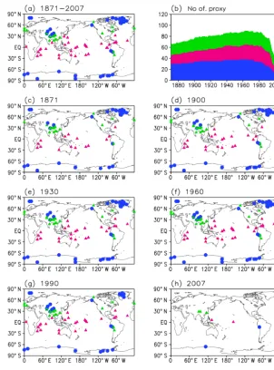
Observations were generated by adding Gaussian noise to the truth. The spatial distribution of the observations mim-icked that of the proxies. The spatial distributions of each proxy for various periods are mapped in Fig. 1. As can be seen from the figure, the distributions and the number of proxies varied with time. However, for the sake of simplicity, the distributions of the proxies were assumed to be constant over time in the CTRL experiment (Fig. 1a). The size of the observation errors will be discussed in Sect. 2.4.
The state vector consisted of five variables: surface air temperature and amount of precipitation, as well as the iso-topic composition in precipitation, coral, and tree-ring cellu-lose. The first three variables were obtained from the isotope-enabled GCM, and the other two variables were obtained from the proxy models driven by the output of the GCM.
2.3.2 Real proxy data assimilation
The second (REAL) experiment assimilated proxy data sam-pled in the real world. To mimic realistic conditions, SST and sea-ice concentration data to be used as model forcing were modified from observational to modeled data. In real-ity, there were no direct observations available for the tar-get period of the proxy DA. Therefore, to reliably evaluate the feasibility of proxy DA, the first estimate should be con-structed using modeled SST, as opposed to observed SST. We used SST data from the historical run of the Coupled Model Intercomparison Project Phase 5 (CMIP5; Taylor et al., 2007) from the atmosphere–ocean coupled version of MIROC5 (Watanabe et al., 2010) obtained from the CMIP5 data server (https://esgf-node.llnl.gov/search/cmip5/).
Because the experiment was not an OSSE, a nature run was not necessary.
2.3.3 Sensitivity experiments
Four sensitivity experiments were conducted to test the ro-bustness of the results of the proxy DA. In the first sensitiv-ity experiment (CGCM), the simulation run was constructed from the simulation forced by the modeled SST and sea ice
as in the REAL experiment. The other settings for the simu-lation run were the same as those in the CTRL experiment. The nature run was the same as that of the CTRL experi-ment. Thus, this experiment investigated how the reconstruc-tion skill of the results was decreased by using the simulated SST compared to the CTRL.
In the second sensitivity experiment (VOBS), the experi-mental design was the same as that in the CGCM, except for the number of proxies that were assimilated. In the CGCM experiment, the distribution and number of proxies were set to be constant over time, as in the CTRL experiment. In the VOBS experiment, the distribution and number of proxies varied with time. Thus, this experiment investigated how the reconstruction skill was decreased by changing the number of proxies compared to the CGCM.
In the third sensitivity experiment (T2-Assim), recon-structed surface temperature (Tr) was assimilated. The pur-pose of the experiment was to compare the skill of the re-constructed DA with that of the proxy DA. The experimental design was the same as that in the CTRL experiment, except for the variables that were assimilated. The reconstructed temperature was generated with a linear regression model of Tr=a+b×δ18O, where a and b are coefficients and δ18O is the observed isotope ratio. The coefficients are cali-brated with the observed isotope ratio and the true tempera-ture in the CTRL for the period of 1871 to 1950 (80 years). If the correlation between the isotope ratio and the tempera-ture during the calibration period was not statistically signif-icant (p <0.10), the data were discarded following Mann et al. (2008). This screening process reduced the available data from 94 to 81 grid points.
The final sensitivity (M08) experiment was used to exam-ine the sensitivity to the observation network. The experi-mental design was the same as for the CTRL, except for the spatial distribution of the proxy. The proxy network used in the experiment was the same as that of Mann et al. (2008). We assumed that isotopic information was available for all the sites, even when this was not the case. For example, even if only tree-ring width data were available at some of the sites in Mann et al. (2008), in this experiment we assumed that isotopic data recorded in tree-ring cellulose were available at the site. The number of grids containing observations were 94 and 250 for the CTRL experiment and M08, respectively. The T2-Assim and the M08 were compared with CTRL.
The experimental designs are summarized in Table 1.
2.4 Observation data
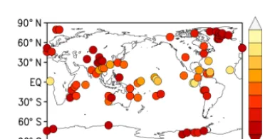
an-Figure 1.Spatial distribution of proxies (δ18O in ice cores, corals, and tree-ring cellulose, denoted by blue, pink, and green, respectively).
(a)Proxies spanning at least 1 year during 1871–2000 are mapped.(b)The number of proxies is depicted as a function of time.(c–h)The spatial distributions of the proxies are mapped for(c)1871,(d)1900,(e)1930,(f)1960,(g)1990, and(h)2007.
nual; proxies whose resolution was lower than annual were excluded. The full list of proxies used in this study is given in the Supplement. Following Crespin et al. (2009) and Goosse et al. (2010), all proxy records were first normalized and then averaged onto a T42 grid box to eliminate model bias and produce a regional grid box composite. To compare the re-sults from each experiment effectively, the assimilated vari-ables were all normalized in both the simulation and nature runs, as well as in the observations in all the experiments.
Errors were added to the truth in a normalized manner to provide the observation for all the experiment other than REAL. The normalized error was uniformly set to 0.50 for all the proxies. This was based on the measurement error of δ18O in ice cores being reported to range from 0.05 to 0.2 ‰ (e.g., Rhodes et al., 2012; Takeuchi et al., 2014), and the
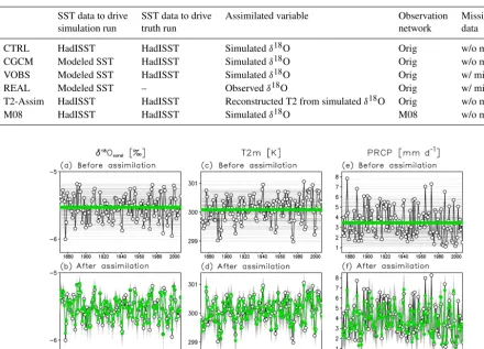
Table 1.Experimental designs. The observation network used in the CTRL experiment is denoted as Orig.
SST data to drive SST data to drive Assimilated variable Observation Missing
simulation run truth run network data
CTRL HadISST HadISST Simulatedδ18O Orig w/o missing
CGCM Modeled SST HadISST Simulatedδ18O Orig w/o missing
VOBS Modeled SST HadISST Simulatedδ18O Orig w/ missing
REAL Modeled SST – Observedδ18O Orig w/ missing
T2-Assim HadISST HadISST Reconstructed T2 from simulatedδ18O Orig w/o missing
M08 HadISST HadISST Simulatedδ18O M08 w/o missing
Figure 2.Annual meanδ18O in corals at a location where observational data were available (1◦N, 157◦W) for(a)background and(b) anal-ysis. The black line indicates the truth, gray lines indicate ensemble members, and green line indicates the ensemble mean.
the proxies. The corresponding signal-to-noise ratio (SNR) is 2.0. The errors are assumed to be independent for all the experiments.
3 Results from the OSSE
The time series of the first estimation, the analysis, and the truth for δ18O in corals are compared as an example in Fig. 2 at a location where observational data were available (1◦N, 157◦W). Because the first estimate was the same for all reconstruction years, it is drawn as horizontal lines. Af-ter the assimilation, the analysis agreed well with the truth (R=0.96,p <0.001). This confirmed that the assimilation performed well. We then examined how accurately the other variables were reconstructed by assimilating isotopic infor-mation. Figure 2 also shows the time series of surface air temperature and precipitation for the same site. There was a clear agreement between the analysis and the truth for both variables (R=0.92 and 0.88, respectively, for temperature and precipitation). This indicated that temperature and pre-cipitation were effectively reconstructed by assimilating iso-topic variables at this site. This was because the isotope ratio
in corals has a signature not only from temperature as given in Eq. (1) but also precipitation (Liu et al., 2013); the correla-tion withδ18Ocoralwas−0.88 (p <0.001) for both tempera-ture and precipitation, respectively. This example shows that the isotopic proxy records more than one variable.
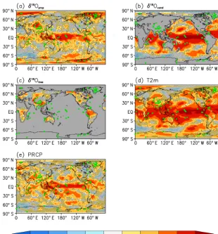
Figure 3 maps the correlation coefficients between the analysis and the truth for the isotope ratio, temperature, and precipitation for 1970–1999. Because the first estimate was constant over time, the temporal correlation between the first estimate and the truth was zero everywhere. Thus, a positive correlation indicated that the DA improved the simulation.
observa-Figure 3.Temporal correlation between the analysis and the truth. The green dots represent the location of the proxy sampling site. The hatched areas indicate where the correlation is not statistically significant (p >0.05).
tion sites in high latitude. In contrast, closely correlated areas were restricted to low latitude for precipitation.
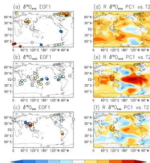
How can the spatial distribution of the correlation pattern be explained; i.e., what do the proxies represent? To investi-gate this question, empirical orthogonal function (EOF) anal-ysis was conducted for the simulatedδ18O in precipitation, corals, and tree-ring cellulose. Only grids that contained ob-servations were included in the analysis. The variables were centered around their means before the analysis. The data covered the period 1871–2007. The EOF patterns and tempo-ral correlations between surface temperature and the charac-teristic evolution of EOF or the principal components (PCs) of the first mode of each proxy are shown in Fig. 4.
The first mode ofδ18O in ice core explains 14.3 % of the total variance and it is the only significant mode according to North et al.’s (1982) rule of thumb (the first and the second mode were indistinguishable). The maximum loadings were in Greenland and Antarctica, where temperature increase has been observed for the past hundred years (e.g., Hartmann et al., 2013). Indeed, the PC1 shows the significant trend and is correlated with global mean surface temperature (R=0.44, p <0.001). Therefore, it is legitimate to regard ice core data
as a proxy of global temperature as revealed from observa-tion (Schneider and Noone, 2007).
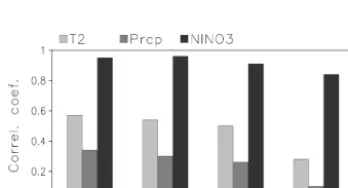
Figure 4.First mode of EOF and the correlation between PC1 and temperature for(a, d)ice cores,(b, e)corals, and(c, f)tree-ring cellulose.
in summer monsoon rainfall in India, which leads to dry con-ditions in summer. The decrease in precipitation leads to iso-topically enriched precipitation, and the dry conditions en-hance the enrichment of water in leaves. Correspondingly, theδ18O in tree-ring cellulose becomes heavier than normal in the positive phase of ENSO. Due to the relationships be-tween the coral and tree-ring cellulose data and ENSO, the correlation coefficient between the analysis and the truth for the NINO3 index was as high as 0.95 (p <0.001).
Although EOF analysis did not reveal any other signifi-cant correlation between PCs and climate indices, climate in-dices for the North Atlantic Oscillation and Southern Annu-lar Mode calculated using the reconstructed data were signif-icantly correlated with the truth (0.59 and 0.46, respectively).
4 Real proxy data assimilation
Based on the results of the idealized experiment described in the previous section, we performed a “real” proxy DA, in which sampled and measured data in the real world were assimilated.
The temporal correlation between the analysis and obser-vations for temperature and precipitation are shown in Fig. 5d
and h. The observations were obtained from HadCRUT3 (Brohan et al., 2006) for temperature, and GHCN-Monthly Version 3 (Peterson and Vose, 1997) for precipitation.
Although the real proxy DA had reasonable skill, it was in-ferior relative to the CTRL experiment. We investigated the cause of the decreased skill using the outputs of the sensitiv-ity experiments. The design of the experiments was changed in a stepwise fashion to more realistic conditions of proxy data assimilation from the idealized conditions. The correla-tions between the analysis and the truth, or the observation, for the experiments are shown in Fig. 5. The truths for the CGCM and VOBS experiments were the same as those for the CTRL experiment. The global mean correlation coeffi-cients for temperature, precipitation, and NINO3 in the ex-periments are summarized in Fig. 6. Note that the correlation was averaged in the same domain for all the experiments to take into account the differences in representativeness.
Figure 5.Temporal correlation between the analysis and the truth for(a–d)temperature and(e–h)precipitation, for each experiment. The green dots represent the location of the proxy sampling site. The hatched areas indicate where the correlation is not statistically significant (p >0.05).
Figure 6.Temporal correlation between the analysis and the truth for each experiment for 1970–1999. The values for temperature and precipitation are the global mean of the temporal correlations.
ENSO measured by the NINO3 index, and the spatial pat-terns of the temperature and precipitation fields regressed on the NINO3 time series (see Figs. 13 and 14 in their report).
Figure 7.Temporal correlations between the analysis and the truth for(a, c)temperature and(b, d)precipitation, for(a, b)CTRL and(b, d)T2-Assim. The green dots represent the location of the proxy sampling site. The hatched areas mean that the correlation is not statistically significant (p >0.05).
When the REAL and VOBS experiments were compared, the correlation coefficients for temperature were significantly decreased over the Indian Ocean, eastern Pacific, and At-lantic Ocean. These areas corresponded to areas of low re-producibility in the coral model (Liu et al., 2014). The ef-fects of sea current and river flow in these areas, which were not included in the coral model, were deemed to be consider-able. Although we cannot attribute all the decreased skill to the coral model, the reproducibility ofδ18O in corals in these areas requires improvement to enhance the performance of the assimilation.
5 Discussion
5.1 Comparison with the reconstructed temperature assimilation
Hughes and Ammann (2009) recommended assimilating measured proxy data, as opposed to reconstructed data de-rived from the proxy data. This subsection compares the re-sults from the CTRL and T2-Assim experiments.
Figure 7 shows the spatial distribution of the correlation coefficients for temperature and precipitation between the truth and the analysis for each experiment. As a whole, the reconstruction skill was slightly degraded in T2-Assim com-pared with CTRL with the global mean correlation coef-ficients for temperature (precipitation) of 0.50 (0.30), 0.45 (0.23), for CTRL and T2-Assim, respectively. On the other hand, the skill of proxy DA was not always better than that
Figure 8.Signal-to-noise ratio (SNR) of the reconstructed temper-ature from the observation used in CTRL.
T2-Figure 9.Temporal correlations in North America between the analysis and the truth for(a, b)temperature, and(c, d)precipitation, for experiments using different proxy networks. The green dots represent the location of the proxy sampling site. The hatched areas indicate where the correlation is not statistically significant (p >0.05).
Assim, and this resulted in the improved skill. Note that the screening process hardly hampered the reconstruction skill, because even if the reconstructed temperature was fully used (i.e., not screened), the skill was almost the same as T2-Assim.
Conducting similar experiments, Dee et al. (2016) also concluded that the reconstruction skill was almost the same among proxy DA and reconstructed DA if the relation be-tween the reconstructed variable and the proxy is linear. As isotope-enabled GCMs (Schmidt et al., 2007; LeGrande and Schmidt, 2009) and observations and models for tree-ring width (D’Arrigo et al., 2008; Evans et al., 2014; Dee et al., 2016) have demonstrated, however, the relations between the proxies and climate are nonlinear and non-stationary as well. Thus, it is difficult to expect that the skill of reconstructed DA will be the same as that of proxy DA if we have the well-defined forward proxy models (Hughes and Ammann, 2009). Although the current models are far from perfect as implied in Sect. 4.2, the assimilation of proxy data will offer a useful tool for the reconstruction of paleoclimate, in which the re-lationship between the proxies and climate constructed with the present-day conditions does not apply.
5.2 Sensitivity to the distribution of the proxies
The skill of the proxy DA was relatively low over Eurasia and North America, even in the idealized experiment. It was unclear whether this was because of limitations in the proxy data assimilation or the scant distribution of the proxies. This subsection investigates the reasons for the relatively low
re-producibility in these areas by comparing the results of the CTRL and M08 experiments, focusing on North America. The number of grids for which proxy data were available over North America was 11 and 126 for the CTRL and M08, respectively.
The results for North America are shown in Fig. 9. The fig-ure shows the temporal correlation coefficients between the analysis and the truth for surface air temperature and pre-cipitation. The correlation coefficients were calculated for 1970–1999. The skill was high in the area in which the prox-ies were densely distributed for both variables. The values of the coefficients averaged over the United States (30–50◦N,
80–120◦W) were 0.69 and 0.58 for temperature and
precipi-tation, respectively. Compared to the coefficients of 0.23 and 0.21, respectively, in the CTRL experiment, the skill was en-hanced for both variables. This implies that the performance of the reconstruction was strongly dependent on the distribu-tion of the proxy data. Taking into consideradistribu-tion that proxy DA can assimilate not only proxy data but also reconstructed data, proxy DA can take advantage of the use of increasingly large amounts of data. Although it is beyond the scope of this study, the combined use of these data is expected to improve the performance of proxy DA.
6 Conclusion and summary
temperature and precipitation in these regions, and the cor-relation between ENSO and δ18O in corals in Pacific and tree-ring cellulose in Tibet. Encouraged by the results, real proxy DA was performed, where the simulation run was con-structed from the simulation forced by the modeled SST, and the real (observed) proxy data were assimilated into the sim-ulation (REAL experiment). The skill of the reconstruction decreased compared to CTRL.
To investigate the reason for the relatively low skill in REAL compared to CTRL, we performed additional experi-ments: CGCM and VOBS. The imperfect SST used to drive the CGCM experiment resulted in a slight reduction of the skill compared to the CTRL experiment with perfect SST. This was because ENSO, which is the most important mode for the reconstruction, was well represented in the modeled SST. The result is encouraging because to apply the DA sys-tem to reconstruct ages where no instrumental observation is available, we must rely on SST simulated by a coupled GCM. Similarly, assimilating the unfixed number of the observation only slightly decreased the reconstruction skill as shown in the comparison between CGCM and VOBS.
From the suite of experiments, more than half of the differ-ence between CTRL and REAL remained unexplained. This remaining difference can have a lot of origins: e.g., errors in the isotope-incorporated atmospheric GCM, the proxy mod-els, and the proxy data. The errors in the models include model biases and missing or overly simplified model com-ponents. For instance, the coral model does not take into ac-count the impact of ocean current or river runoff in this study. Furthermore, post-depositional processes for simulating iso-tope ratio in ice core were not included at all. Those pro-cesses should be included to enable more efficient utilization of all the data. The errors in proxy data include misrepresen-tation of the targeted temporal and/or spatial scales. It is also possible that the data were highly distorted by non-climatic factors. Thus, a thorough quality control, similar to the pro-cedures used in weather forecasting, should be conducted be-fore assimilation (e.g., Appendix B of Compo et al., 2011). At this stage, it is difficult to show the relative contributions of each factor to the degraded skill in REAL, it is necessary to estimate the impact of structural errors in models as done in Dee et al. (2016).
Although the skill of proxy DA is dependent on the repro-ducibility of the models and the number and quality of the observations, the results suggest that it is feasible to constrain climate using only proxies. In particular, ENSO and ENSO-related variations in temperature and precipitation should be reliably reconstructed even with the current proxy DA sys-tem and proxy network used in this study because the corre-lation coefficient between the analysis and the observations was as high as 0.83 in the REAL experiment. Although the reconstruction of ENSO is dependent on data from corals, and the time span covered by corals is relatively short (a few hundred years), ENSO can still be reliably reconstructed due
to its global impact, as was demonstrated in the relationship between isotopes in tree-ring cellulose from Tibet.
Moreover, we expect that the reproducibility will increase as more proxy data become available because it was heavily dependent on the spatial distribution. Given that proxy DA can assimilate both proxy data and data reconstructed from proxy, and that the reconstruction skill in reconstructed DA is slightly superior to proxy DA, the combined use of the two types of data is beneficial for the performance. In that case, care must be taken not to assimilate dependent informa-tion (e.g., proxy data and reconstructed data from the same proxy).
The DA algorithm used in this study did not consider non-stationarity among proxies and climate variables because the Kalman gain was constant over time. To address non-stationarity, the Kalman gain for a specific reconstruction year should be constructed for several tens of years before and after that year. Nevertheless, EnKF can only capture linear relationships between observations and the modeled state. The use of other algorithms, such as particle filter (e.g., van Leeuwen, 2009), or four-dimensional variational assim-ilation (e.g., Rabier et al., 2000) should be investigated in future studies for scenarios where nonlinearity is not neg-ligible. Thus, it is important in future studies to investigate non-stationarity and nonlinearity among proxies and climate variables to identify suitable algorithms for proxy DA.
Data availability. Data for this paper are accessible through the Supplement.
The Supplement related to this article is available online at doi:10.5194/cp-13-379-2017-supplement.
Competing interests. The authors declare that they have no con-flict of interest.
Acknowledgements. The first author was supported by the Japan Society for the Promotion of Science (JSPS) via a Grant-in-Aid for JSPS Fellows. This study was supported by the Japan Society for the Promotion of Science (grants 15H01729, 26289160, and 23226012), the SOUSEI Program, the ArCS project of MEXT, Project S-12 of the Japanese Ministry of the Environment, and the CREST program of the Japan Science and Technology Agency.
Edited by: V. Rath
Reviewed by: two anonymous referees
References
Acevedo, W., Fallah, B., Reich, S., and Cubasch, U.: Assimilation of Pseudo-Tree-Ring-Width observations into an Atmospheric General Circulation Model, Clim. Past Discuss., doi:10.5194/cp-2016-92, in review, 2016b.
Annan, J. D. and Hargreaves, J. C.: Identification of climatic state with limited proxy data, Clim. Past, 8, 1141–1151, doi:10.5194/cp-8-1141-2012, 2012.
Asami, R., Yamada, T., Iryu, Y., Meyer, C. P., Quinn, T. M., and Paulay, G.: Carbon and oxygen isotopic composition of a Guam coral and their relationships to environmental variables in the western Pacific, Palaeogeogr. Palaeocl., 212, 1–22, 2004. Bhend, J., Franke, J., Folini, D., Wild, M., and Brönnimann, S.: An
ensemble-based approach to climate reconstructions, Clim. Past, 8, 963–976, doi:10.5194/cp-8-963-2012, 2012.
Brohan, P., Kennedy, J. J., Harris, I., Tett, S. F. B., and Jones, P. D., Uncertainty estimates in regional and global observed tempera-ture changes: A new data asset from 1850, J. Geophys. Res., 111, D12106, doi:10.1029/2005JD006548, 2006.
Brown, J., Simmonds, I., and Noone, D.: Modelingδ18O in tropical precipitation and the surface ocean for present-day climate, J. Geophys. Res., 111, D05105, doi:10.1029/2004JD005611, 2006. Compo, G. P., Whitaker, J. S., Sardeshmukh, P. D., Matsui, N., Al-lan, R. J., Yin, X., Gleason Jr., B. E, Vose, R. S., Rutledge, G., Bessemoulin, P., Brönnimann, S., Brunet, M., Crouthamel, R. I., Grnt, A. N., Groisman, P. Y., Jones, P. D., Kruk, M. C., Kruger, A. C., Marshall, G. J., Maugeri, M., Mok, H. Y., Nordli, Ø., Ross, T. F., Trigo, R. M., Wang, X. L., Woodruff, S. D., and Worley, S. J., The twentieth Century Reanalysis Project, Q. J. Roy. Meteor. Soc., 137, 1–28, 2011.
Crespin, E., Goosse, H., Fichefet, T., and Mann, M. E.: The 15th century Arctic warming in coupled model simulations with data assimilation, Clim. Past, 5, 389–401, doi:10.5194/cp-5-389-2009, 2009.
D’Arrigo, R., Wilson, R., Liepert, B., and Cherubini, P.: On the “Di-vergence Problem” in Northern Forests: A review of the the tree-ring evidence and possible causes, Global Planet. Change, 60, 289–305, 2008.
Dee, S., Emile-Geay, J., Evans, M., Allam, A., Steig, E., and Thompson, D.: PRYSM: An open-source framework for PRoxY System Modeling, with applications to oxygen-isotope systems, Journal of Advances in Modeling Earth Systems, 7, 1220–1247, 2015.
Dee, S., Steiger, N. J., Emile-Geay, J., and Hakim, G. J.: On the util-ity of proxy system models for estimating climate states over the common era, Journal of Advances in Modeling Earth Systems, 8, 1164–1179, 2016.
Dirren, S. and Hakim, C.: Toward the assimilation of time-averaged observations, Geophys. Res. Lett., 32, L04804, doi:10.1029/2004GL021444, 2005.
Dubinkina, S. and Goosse, H.: An assessment of particle filtering methods and nudging for climate state reconstructions, Clim. Past, 9, 1141–1152, doi:10.5194/cp-9-1141-2013, 2013. Epstein, S. and Mayeda, T.: Variation of O18content of waters from
natural sources, Geochim. Cosmochim. Ac., 4, 213–224, 1953. Evans, M. N., Tolwinski-Ward, S. E., Thompson, D. M., and
An-chukaitis, K. J.: Applications of proxy system modeling in high resolution paleoclimatology, Quaternary Sci. Rev., 76, 16–28, 2013.
Evans, M. N., Smerdon, J. E., Kaplan, A., Tolwinski-Ward, S. E., and González-Rouco, J. F.: Climate field reconstruc-tion uncertainty arising from multivariate and nonlinear prop-erties of predictors, Goephys. Res. Lett., 41, 9127–9134, doi:10.1002/2014GL062063, 2014.
Gaspari, G. and Cohn, S.: Construction of correlation functions in two and three dimensions, Q. J. Roy. Meteor. Soc., 125, 723–757, 1999.
Goodkin, N. F., Hughen, K. A., Curry, W. B., Doney, S. C., and Os-termann, D. R.: Sea surface temperature and salinity variability at Bermuda during the end of the Little Ice Age, Paleoceanography, 23, PA3203, doi:10.1029/2007PA001532, 2008.
Goosse, H., Renssen, H., Timmermann, A., Bradley, R., and Mann, M.: Using paleoclimate proxy-data to select optimal realisations in an ensemble of simulations of the climate of the past millen-nium, Clim. Dynam., 27, 165–184, 2006.
Goosse, H., Crespin, E., de Montety, A., Mann, M., Renssen, H., and Timmermann, A.: Reconstructing surface temperature changes over the past 600 years using climate model simula-tions with data assimilation, J. Geophys. Res., 115, D09108, doi:10.1029/2009JD012737, 2010.
Goosse, H., Crespin, E., Dubinkina, S., Loutre, M., Mann, M., Renssen, H., Sallaz-Damaz, Y., and Shindell, D.: The role of forcing and internal dynamics in explaining the “Medieval Cli-mate Anomaly”, Clim. Dynam., 39, 2847–2866, 2012.
Hartmann, D. L., Klein Tank, A. M. G., Rusticucci, M., Alexan-der, L. V., Brönnimann, S., Charabi, F., Dentener, F. J., Dlugo-kencky, E. J., Easterling, D. R., Kaplan, A., Soden, B. J., Thorne, P. W., Wild, M., and Zhai, P. M.: Observations: Atmosphere and Surface, in: Climate Change 2013: The physical science basis. Contribution of Working Group I to the Fifth Assessment Re-port of the Intergovernmental Panel on Climate Change, Cam-bridge University Press, CamCam-bridge, UK and New York, NY, USA, 2013.
Hoffmann, G., Werner, M., and Heimann, M.: Water isotope module of the ECHAM atmospheric general circulation model: A study on timescales from days to several years, J. Geophys. Res., 103, 16871–16896, 1998.
Houtekamer, P. L. and Zhang, F., Review of the ensemble Kalman filter for atmospheric data assimilation, Mon. Weather Rev., 144, 4489–4532, 2016.
Hughes, M. and Ammann, C.: The future of the past – an earth system framework for high resolution paleoclimatology: edito-rial essay, Climatic Change, 94, 247–259, 2009.
Huntley, H. and Hakim, G.: Assimilation of time-average observa-tions in a quasi-geostrophic atmospheric jet model, Clim. Dy-nam., 35, 995–1009, 2010.
Joussaume, S., Sadourny, R., and Jouzel, J.: A general circulation model of water isotope cycles in the atmosphere, Nature, 311, 24–29, 1984.
Jouzel, J., Russell, G. L., Suozzo, R. J., Koster, R. D., White, J. W. C., and Broecker, W. S.: Simulations of the HDO and H182 O Atmospheric cycles using the NASA GISS General Circulation Model: The seasonal cycle for present-day conditions, J. Geo-phys. Res., 92, 14739–14760, 1987.
Lee, J.-E., Fung, I., DePaolo, D., and Henning, C.: Analysis of the global distribution of water isotopes using the NCAR at-mospheric general circulation model, J. Geophys, Res., 112, D16306, doi:10.1029/2006JD007657, 2007.
LeGrande, A. and Schmidt, G.: Global gridded data set of the oxy-gen isotopic composition in seawater, Geophys. Res. Lett., 33, L12604, doi:10.1029/2006GL026011, 2006.
LeGrande, A. N. and Schmidt, G. A.: Sources of Holocene variabil-ity of oxygen isotopes in paleoclimate archives, Clim. Past, 5, 441–455, doi:10.5194/cp-5-441-2009, 2009.
Liu, G., Kojima, K., Yoshimura, K., Okai, T, Suzuki, A., Oki, T., Siringan, F., Yoneda, M., and Kawahata, H.: A model-based test of accuracy of seawater oxygen isotope ratio record derived from a coral dual proxy method at southeastern Luzon Island, the Philippines, J. Geophys. Res.-Biogeo., 118, 853–859, 2013. Liu, G., Kojima, K., Yoshimura, K., and Oka, A.: Proxy
interpretation of coral-recorded seawater 18O using 1-D model forced by isotope-incorporated GCM in tropical oceanic regions, J. Geophys. Res.-Atmos., 119, 12021–12033, doi:10.1002/2014JD021583, 2014.
Managave, S. R., Sheshshayee, M. S., Ramesh, R., Borgaonkar, H. P., Shad, S. K., and Bhattacharyya, A.: Response of cellulose oxygen isotope values of teak trees in differing monsoon environ-ments to monsoon rainfall, Dendrochronologia, 29, 89–97, 2011. Mann, M., Zhang, Z., Hughes, M., Bradley, R., Miller, S., Ruther-ford, S., and Ni, F.: Proxy-based reconstructions of hemispheric and global surface temperature variations over the past two mil-lennia, P. Natl. Acad. Sci. USA, 105, 13252–13257, 2008. Mathiot, P., Goosse, H., Crosta, X., Stenni, B., Braida, M., Renssen,
H., Van Meerbeeck, C. J., Masson-Delmotte, V., Mairesse, A., and Dubinkina, S.: Using data assimilation to investigate the causes of Southern Hemisphere high latitude cooling from 10 to 8 ka BP, Clim. Past, 9, 887–901, doi:10.5194/cp-9-887-2013, 2013.
Noone, D. and Simoonds, I., Associations betweenδ18O of water and climate parameters in a simulation of atmospheric circulation for 1979–95, J. Climate, 15, 3150–3169, 2002.
North, G., Bell, T. L., and Cahalan, R. F., Sampling errors in the es-timation of empirical orthogonal functions, Mon. Weather Rev., 110, 699–706, 1982.
Okazaki, A. and Yoshimura, K.: Development of stable water iso-tope incorporated atmosphere-land coupled model MIROC5, in preparation, 2017.
PAGES 2k Consortium, Continental-scale temperature variability during the past wto millennia, Nat. Geosci., 6, 339–346, 2013. Peterson, T. C. and Vose, R. S.: An overview of the global
histori-cal climatology network temperature database, B. Am. Meteorol. Soc., 78, 2837–2849, 1997.
Rabier, F., Järvinen, H., Klinker, E., Mahfouf, J.-F., and Sim-mons, A.: The ECMWF operational implementation of four-dimensional variational assimilation. I: Experimental results with simplified physics, Q. J. Roy. Meteor. Soc., 126, 1143–1170, 2000.
Rasmusson, E. M. and Capenter, T. H.: The relationship between eastern Equatorial Pacific sea surface temperatures and rainfall over India and Sri Lanka, Mon. Weather Rev., 111, 517–528, 1983.
Rayner, N. A., Parker, D. E., Horton, E. B., Folland, C. K., Alexan-der, L. V., Rowell, D. P., Kent, E. C., and Kaplan, A.: Global
analyses of sea surface temperature, sea ice, and night marine air temperature since the late nineteenth century, J. Geophys. Res., 108, D144407, doi:10.1029/2002JD002670, 2003.
Rhodes, R. H., Bertler, N. A. N., Baker, J. A., Steen-Larsen, H. C., Sneed, S. B., Morgenstern, U., and Johnsen, S. J.: Little Ice Age climate and oceanic conditions of the Ross Sea, Antarc-tica from a coastal ice core record, Clim. Past, 8, 1223–1238, doi:10.5194/cp-8-1223-2012, 2012.
Risi, C., Bony, S., Vimeux, F., and Jouzel, J.: Water-stable isotopes in the LMDZ4 general circulation model: Model evaluation for present-day and past climates and applications to climatic in-terpretations of tropical isotopic records, J. Geophys. Res., 115, D12118, doi:10.1029/2009JD013255, 2010.
Roden, J., Lin, G., and Ehleringer, J.: A mechanistic model for in-terpretation of hydrogen and oxygen isotope ratios in tree-ring cellulose, Geochim. Cosmochim. Ac., 64, 21–35, 2000. Sano, M., Xu, C., and Nakatsuka, T.: A 300-year
Viet-nam hydroclimate and ENSO variability record reconstructed from tree ring δ18O, J. Geophys. Res., 117, D12115, doi:10.1029/2012JD017749, 2012.
Schmidt, G., Hoffmann, G., Shindell, D., and Hu, Y.: Modeling atmospheric stable isotopes and the potential for constraining cloud processes and staratosphere-troposphere water exchange, J. Geophys. Res., 110, D21314, doi:10.1029/2005JD005790, 2005.
Schmidt, G., LeGrande, A., and Hoffmann, G.: Water iso-tope expressions of intrinsic and forced variability in cou-pled ocean-atmosphere model, J. Geophys. Res., 112, D10103, doi:10.1029/2006JD007781, 2007.
Schneider, D. P. and Noone, D. C.: Spatial covariance of wa-ter isotope records in a global netweok of ice cores span-ning twentieth-century climate change, J. Geophys. Res., 112, D18105, doi:10.1029/2007JD008652, 2007.
Schotterer, U., Stichler, W., and Ginot, P.: The influence of post-depositional effects on ice core studies: Examples from the Alps, Andes, and Altai, in Earth Paleoenvironments: Records Pre-served in Mid- and Low-Latitude Glaciers, 39–59, Kluwer Acad, Dordrecht, the Netherlands, 2004.
Steiger, N., Hakim, G., Steig, E., Battisti, D., and Roe, G.: Assimi-lation of Time-Averaged Pseudoproxies for Climate Reconstruc-tion, J. Climate, 27, 426–441, 2014.
Taylor, K. E., Stouffer, R. J., and Meehl, G.: An overview of CMIP5 and the experiment design, B. Am. Meteorol. Soc., 93, 485–498, 2007.
Takeuchi, N., Fujita, K., Aizen, V. B., Narama, C., Yokoyama, Y., Okamoto, S., Naoki, K., and Kobota, J.: The disappearance of glaciers in the Tien Shan Mountains in Central Asia at the end of Pleistocene, Quaternary Sci. Rev., 103, 26–33, 2014.
Thompson, D. M., Ault, T. R., Evans, M. N., Cole, J. E., and Emile-Geay, J.: Comparison of observed and simulated tropical climate trends using a forward model of coralδ18O, Geophys. Res. Lett., 38, L14706, doi:10.1029/2011GL048224, 2011.
van der Schrier, G. and Barkmeijer, J.: Bjerknes’ hypothesis on the coldness during AD 1790–1820 revisited, Clim. Dynam., 25, 537–553, 2005.
van Leeuwen, P. J.: Particle filtering in geophysical systems, Mon. Weather Rev., 137, 4089–4114, 2009.
eviedence and GCMs by means of data assimilation though up-scaling and nudging (DATUN), Proc. 11th Symposium on Global Climate Change Studies, AMS Long Beach, CA, 2000. Watanabe, M., Suzuki, T., O’ishi, R., Komuro, Y., Watanabe, S.,
Emori, S., Takemura, T., Chikira, M., Ogura, T., Sekiguchi, M., Takata, K., Yamazaki, D., Yokohota, T., Nozawa, T., Hasumi, H., Tatebe, H., and Kimoto, M.: Improved climate simulation by MIROC5: Mean States, Variability, and Climate Sensitivity, J. Climate, 23, 6312–6335, 2010.
Werner, M., Langebroek, P., Carlsen, T., Herold, M., and Lohmann, G.: Stable water isotopes in the ECHAM5 gen-eral circulation model: Toward high-resolution isotope mod-eling on a global scale, J. Geophys. Res., 116, D15109, doi:10.1029/2011JD015681, 2011.
Whitaker, J. S. and Hamill, T. M.: Ensemble data assimilation with-out perturbed observations, Mon. Weather Rev., 130, 1913–1924, 2002.
Widmann, M., Goosse, H., van der Schrier, G., Schnur, R., and Barkmeijer, J.: Using data assimilation to study extratropical Northern Hemisphere climate over the last millennium, Clim. Past, 6, 627–644, doi:10.5194/cp-6-627-2010, 2010.
Xu, C., Sano, M., and Nakatsuka, T.: Tree ring cellulose δ18O of Fokienia hodginsii in northern Laos: A promising proxy to reconstruct ENSO?, J. Geophys. Res., 116, D245109, doi:10.1029/2011JD016694, 2011.
Xu, C., Zheng, H., Nakatsuka, T., and Sano, M.: Oxygen iso-tope signatures preserved in tree ring cellulose as a proxy for April-September precipitation in Fujian, the subtropical region of southeast China, J. Geophys. Res-Atmos., 118, 12805–12815, 2013.
Xu, C., Pumijumnong, N., Nakatsuka, T., Sano, M., and Li, Z.: A tree-ring celluloseδ18O-based July-October precipitation recon-struction since AD 1828, northwest Thailand, J. Hydrol., 529, 422–441, 2015.
Yoshimura, K., Kanamitsu, M., Noone, D., and Oki, T.: Historical isotope simulation using Reanalysis atmospheric data, J. Geo-phys, Res., 113, D19108, doi:10.1029/2008JD010074, 2008. Yoshimura, K., Miyoshi, T., and Kanamitsu, M.: Observation
sys-tem simulation experiments using water vapor isotope informa-tion, J. Goephys, Res., 119, 7842–7862, 2014.