The Evaluation of Forecasting Methods for Sales of Sterilized Flavoured Milk in Chhattisgarh

(1)

ISSN: 2231-5381

http://www.ijettjournal.org

Page 98

The Evaluation of Forecasting Methods for Sales

of Sterilized Flavoured Milk in Chhattisgarh

Pradeep Kumar Sahu#1, Rajesh Kumar*2

#

Assistant Professor Mechanical Department Chhatrapati Shivaji Institute of Technology

Durg, Chhattisgarh, India

Abstract— In recent years, there has been a great deal of discussion on applications of various forecasting models and their performance in forecasting business activities. This paper discussed few of forecasting models and their application for sales forecasting of sterilized flavoured milk in Chhattisgarh. Applying weekly data spreading over October 2011 to October 2012, on the sales of sterilized flavoured milk in liter. The forecasting method analysed included: naϊve model , moving

average, double moving average, simple exponential smoothing; and semi average method. The accuracy of the forecasting method was measured using mean Forecast Error (MFE), mean Absolute Deviation (MAD), mean Square Error (MSE), root mean square Error (RMSE).

Keywords— sterilized flavoured milk, forecasting models

Introduction

Forecasting is defined as the prediction of future events based on known past value of relevant variables (Makridakis,Wheelwright,& Hyndman, 1998).Accurate forecasting is essential for manager to plan effectively. Inaccurate forecasting may lead to bad decisions that may lead, to ineffective management in overall operations.

Over-forecasting also increases the labour cost because the additional handling of product requires additional labour. Under –forecasting lead to the problem of product that runs out before customer demand is satisfied, this results in more immediate concerns. Under-production leads to increased stress for employees and manager who are likely to customer dissatisfaction. Finally, under- forecasting will result in decreased employee morale and manager confidence.

I. LITERATURE SURVEY

There has been a great deal of discussion in economic literature about applications of various forecasting models for forecasting desired issues. Several time series forecasting techniques such as naϊve model, moving average, double moving average, simple exponential smoothing; and semi average method has been applied to forecasting. In a study, Cacatto et al., (2012) introduce the forecasting practices that have been used by food industries in Brazil and detect how

these companies have been used forecasting methods, what are the main factors that influence their choice. The data was analyzed by multivariate statistics techniques using the SPSS software. The result shows that the companies do not use sophisticated forecasting methods: the historical analysis model is the mostly used. The factors that influence the choice of the models are the type of product and the time spent during the forecasting, and the main difficulties is the availability of the appropriate software.

Ryu et al., (2003) evaluated the forecasting method for institutional food service facility. They are identifying the most appropriate forecasting method of forecasting meal count for an institutional food service facility. The forecasting method analyzed included: naϊve model 1,2 and 3; moving average method ,double moving method , exponential smoothing method, double exponential method, Holt’s method, Winter method, linear regression and multiple regression method. The accuracy of forecasting methods was measured using mean absolute deviation, mean squared error, mean percentage error, mean absolute percentage error method, root mean squared error and Theil’s U- statistic. The result of this study showed that multiple regressions was the most accurate forecasting method, but naϊve method 2 was selected as the most appropriate forecasting method because of its simplicity and high level of accuracy.

Alfares et al., (2002) categorized the electric load forecasting technique. A wide range of methodology and model for forecasting are given in literature. These techniques are classified into nine categories: (1) multiple regression, (2) exponential smoothing, (3) iterative reweighted least-squares, (4) adaptive load forecasting, (5) stochastic time series, (6) ARMAX model based on genetic algorithms, (7) fuzzy logic, (8) neural networks and (9) expert systems. The methodology for each category is briefly described, the advantage and disadvantages discussed.

II. DATA COLLECTION

(2)

ISSN: 2231-5381

http://www.ijettjournal.org

Page 99

Week No. Demand Week No. Demand

1 1164.4 29 628.8

2 678.8 30 951.6

3 1384.2 31 1136.8

4 326.4 32 387.2

5 982 33 2055.6

6 681.6 34 676.8

7 792 35 754.8

8 888 36 1974.8

9 1648.4 37 1182

10 566.4 38 471.6

11 465.6 39 868.8

12 288 40 782.4

13 253.6 41 679

14 225.6 42 203.6

15 1219.8 43 142.2

16 280 44 135.2

17 254.4 45 1174.4

18 206.4 46 548

19 468.6 47 184.6

20 1128 48 1661.6

21 969.6 49 267.2

22 641 50 1611

23 960 51 802.2

24 1113.6 52 469.6

25 2367.2 53 374.4

26 1317.2 54 1042.2

27 1305.6 55 1136.8

28 1382 56 438

Table 1: Demand of Sterilized flavoured Milk (in liter)

Fig 1: Demand of Sterilized flavoured Milk (in liter)

III.METHODOLOGY

This study evaluated different forecasting model using sterilized flavoured milk demand data from Raipur dugdh sangh (Devbhog) at Raipur (Chhattisgarh).Weekly data from October 2011 to October 2012 were collected and used to forecast the sterilized flavoured milk demand. The forecast model used in the analysis included simple moving average method (n=2, n=3, n=4), double moving average method(n=2, n=3, n=4), single exponential method (α=0.1, α=0.2, α=0.3), semi average method, naϊve Model. The most appropriate forecasting method was determined on the basis of accuracy. In this research, several common accuracy methods were used: mean forecast error (MFE), mean absolute deviation (MAD), mean square error (MSE) and root mean square error (RMSE). The ranking was assigned to each forecasting method.

A. Forecasting Methods

1) Moving Average Method. The moving average method

involves calculating the average of observations and then employing that average as the predictor for the next period. The moving average method is highly dependent on n, the number of terms selected for constructing the average. The equation is as follows:

Ft+1 = (Yt +Yt-1 +Yt-2 + ……+Yt-n+1)/n

Where:

Ft+1 = the forecast value for the next period

Yt = the actual value at period t

n = the number of term in the moving average

(3)

ISSN: 2231-5381

http://www.ijettjournal.org

Page 100

has been to use MSE. In this study, the value of n taking 2, 3,

and 4.

2) Double Moving Average Method: Hanke and Reitsch

(1998) recommended the use of the double moving average method to forecast time series data. Forecasting with a double moving average requires determining two averages. The first moving average is computed; a second moving average is calculated. Five equations are used in the double moving average:

Mt = Ft+1 = (Yt +Yt-1 +Yt-2 + ……+Yt-n+1)/n

M’t = (Mt + Mt-1 +Mt-2 + ……+Mt-n+1)/n

At = 2Mt - M’t

Bt =

1

2 

n

( Mt - M ’

t )

Ft+p = At + Bt p

Where:

n = the number of period in the double moving average

Yt = the actual series value at time period t

P = the number of period ahead to be forecast

3) Simple Exponential Smoothing Method: The

exponential smoothing method is a technique that uses a weighted moving average of past data as the basis for a forecast. This method keeps a running average of demand and adjusts it for each period in proportion to the difference between the latest actual demand figure and the latest value of the average. The equation for the simple exponential smoothing method is:

Ft+1 = α Yt + (1-α) Ft-1

Where:

Ft+1 = the new smoothing value or the forecast value for

the next period

α= the smoothing constant (0 < α <1)

Yt = the new observation or actual value of the series in

period t

Ft = the old smoothed value or forecast for period t

The accuracy of the simple exponential smoothing method strongly depended on the optimal value of (α).The preferred range for α is from 0.1 to 0.3. In this study, the value of α taking 0.1, 0.2 and 0.3.

4) Semi – Average Method: According to this method,

the original data are divided into two equal parts and the values of each part are then summed up and averaged. The average of each part is centered in the period of the time of the part from which it has been calculated and then plotted on graph. Then a straight line is drawn to pass through the plotted points. This line constitutes the semi – average trend line. When the number of year is odd, the middle year is not considered while dividing the data into two equal parts and obtaining the average.

5) Naϊve Method: Naϊve method are forecasting

techniques obtained with a minimal amount of effort and data manipulation and are based on the most recent information available (Shim, 2000). The naϊve method uses data from the previous week to forecast the current week (one week lag):

Ft+1 = Yt

Where:

Ft+1 = the forecast value for the next period

Yt = the actual value at the next period

B. Measuring Forecasting Error

1) Mean Forecast Error: Mean forecast error (MFE) is

the mean of the deviation of the forecast demands from the actual demands.

MFE =

n

F

Y

_t

n

t

)

(

1







Where:

Yt = the actual value in time period t

Ft = the forecast value in time period t

n = the number of periods

2) Mean Absolute Deviation: A common method for

Measuring overall forecast error is the mean absolute deviation (MAD). Heizer and Render (2001) noted that this value is computed by dividing the sum of the absolute values of the individual forecast error by the sample size (the number of forecast periods). The equation is:

MAD =

n

F

Y

_t

n

t

)

(

1







(4)

ISSN: 2231-5381

http://www.ijettjournal.org

Page 101

3) Mean Square Error: Jarrett (1991) stated that the

mean square error (MSE) is a generally accepted technique for evaluating exponential smoothing and other methods. The equation is:

MSE = 2

1

)

(

1

t n

t

F

Y

n







Where:

4) Root Mean Square Error:Root mean square error

(RMSE) is the square root of MSE. This measures error in term of units that are equal to the original value (Jarrett, 1991).Symbolically, the equation is:

RMSE =

1 (

)

1







n

t

t t

F

Y

n

Where:

C. Evaluation of Forecasting Method

In this study, the most appropriate forecasting method was selected on the basis of both level of accuracy and ease of use. The various forecasting method are using to forecast future demand of sterilized flavored milk in Chhattisgarh, the accuracy of the forecasting method was assessed using mean forecast error (MFE), mean absolute deviation (MAD), mean square error (MSE), and root mean square error (RMSE).

In the case of forecasting of sterilized flavored milk demand in Chhattisgarh, special consideration as to each method’s ease of use was required, since the person in charge of forecasting usually has little time and-in some instances- little knowledge of how implement the forecasts.

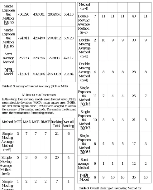
METHOD

MFE

MAD

MSE

RMSE

Simple

Moving

Average

Method

(n=2)

-4.54

458.296 345991

588.21 Simple

Moving

Average

Method

(n=3)

-12.171 427.686

292891

541.19 Simple

Moving

Average

Method

(n=4)

-1.6027 404.976

285162

534.05 Double

Moving

Average

Method

(n=2)

-15.805 626.588

592155

769.51 Double

Moving

Average

Method

(n=3)

1.9182

552.732 448771

669.90 Double

Moving

Average

Method

(n=4)

6.5897

516.738 446955

668.54 Single

Exponen

tial

Method(

α=0.1)

(5)

ISSN: 2231-5381

http://www.ijettjournal.org

Page 102

Single

Exponen

tial

Method(

α=0.2)

-36.298 432.681 285295.6 534.13

Single

Exponen

tial

Method(

α=0.3)

-24.811 428.490 290745.2 539.20

Semi

average

Method

25.273

328.356 223898

473.17 Naϊve

Model

-12.971 532.264 495390.9 703.84

Table 2: Summary of Forecast Accuracy (St.Flav.Milk)

IV.RESULT AND DISCUSSION

In this study, four accuracy model- mean forecast error (MFE), mean absolute deviation (MAD), mean square error (MSE), and root mean square error (RMSE)-were adopted to assess the accuracy of forecasting methods. The smaller the forecast error, the more accurate forecasting method.

Method MFE MAD MSE RMSE Ranking

Total

Over-all

Ranking

Simple

Moving

Average

Method

(n=2)

3

7

24

6 Simple

Moving

Average

Method

(n=3)

5

3

6

20

4 Simple

Moving

Average

1

2

7

1 Method

(n=4)

Double

Moving

Average

Method

(n=2)

7

11

40

11 Double

Moving

Average

Method

(n=3)

2

10

9

30

9 Double

Moving

Average

Method

(n=4)

4

8

28

8 Single

Exponen

tial

Method

(α=0.1)

11

7

4

25

7 Single

Exponen

tial

Method

(α=0.2)

10

5

3

21

5 Single

Exponen

tial

Method

(α=0.3)

8

4

5

17

3 Semi

average

Method

9

1

12

2 Naϊve

Model

6

9

10

35

10

(6)

ISSN: 2231-5381

http://www.ijettjournal.org

Page 103

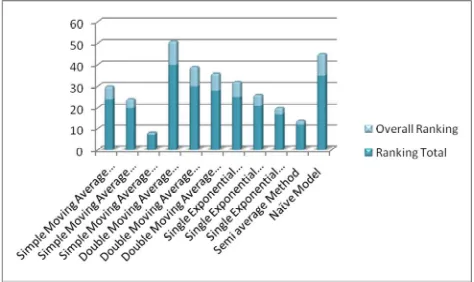
Simple Moving Average Method (n=4) was ranked first

because it had small errors and the total ranking of the Simple Moving Average Method (n=4) is 7 as shown in Table 3and Fig.2. In this method (MFE=-1.6027, MAD=404.976, MSE=285162, RMSE=534.005) outperformed all the other methods.

Semi average Method was ranked second because the total ranking of this method is 12 as shown in Table 3 and Fig.2. Semi average Method obtained the second minimum errors (MFE= 25.273, MAD = 328.356, MSE = 223898, RMSE = 473.179) as shown in Table 2.

Single Exponential Method (α=0.3) was ranked third because total ranking is 17 as shown in Table 3 and Fig.2. Single Exponential Method with α =0.3 produced third smallest error as shown in Table 2.

Simple Moving Average Method (n=3) method produced large errors (MFE= -12.171, MAD = 427.686, MSE = 292891, RMSE = 541.194) as compare to semi average method, Simple Moving Average method (n=4) and Single Exponential Method (α=0.3). So this method ranked is fourth.

Single Exponential Method (α=0.2) was ranked fifth because it had large errors (MFE = -36.298, MAD = 432.6811, MSE = 285295.6, RMSE = 534.1307) and total ranking is 21 as shown in Table 3 and Fig.2.

Simple Moving Average Method (n=2) was ranked sixth because the total ranking of this method is 24 as shown in Table 3 and Fig.2. Simple Moving Average Method (n=2) obtained the sixth minimum errors (MFE= -4.54, MAD = 458.296, MSE = 345991, RMSE = 588.21) as shown in Table 2.

Single Exponential Method (α=0.1) was ranked seventh because it had large errors (MFE = -68.6854, MAD = 451.8034, MSE = 289302.3, RMSE = 537.8683) and total ranking is 25 as shown in Table 3 and Fig.2.

Double Moving Average Method (n=4) was ranked eight because the total ranking of this method is 28 as shown in Table 3. Simple Moving Average Method (n=4) obtained the eight minimum errors (MFE= 6.58973, MAD = 516.738, MSE = 446955, RMSE = 668.547) as shown in Table 2.

Double Moving Average Method (n=3) was ranked ninth because total ranking is 30 as shown in Table 3 and Fig.2. In Double Moving Average Method with n=3 produced ninth smallest error as shown in Table 2.

Naϊve Model using the last week of data to forecast the next week. It has the lag of one week. Naϊve Method had large error (MFE = -12.971, MAD = 532.2643, MSE = 495390.9, RMSE = 703.8401) as shown in Table 2. So this model ranked is tenth.

Double Moving Average Method (n=2) was ranked eleventh because total ranking is 40 as shown in Table 3 and Fig.2. In Double Moving Average Method with n=2 produced maximum error as shown in Table 2.

Fig.2 Graph between ranking total and overall ranking

V. CONCLUSIONS

This study identified the most appropriate forecasting method based on accuracy and simplicity. The result showed that Simple Moving Average Method (n=4) obtained the best accuracy; however, it was selected as the most appropriate forecasting method for sales forecasting of sterilized flavored milk in Chhattisgarh.

REFERENCES

[1] Armstrong, J.S. and Collopy, F., (1992) “Error Measures For Generalizing About Forecasting Method: Empirical Comparisons”, International Journal of Forecasting, Vol.8, pp 69-80.

[2] Armstrong, J.S., & Lusk, E.J., (1983) “The accuracy of alternative extrapolation models: analysis of a forecasting competition through open peer review” Journal of forecasting, Vol.2, Issue 3, pp 259-311.

[3] Armstrong, J.S., et al., (2005) “The forecasting canon: nine generalization to improve forecast accuracy” The international journal of applied forecasting, Vol.1, Issue 1, pp 29-35.

[4] Armstrong, J.S., & Collopy, F., (1992)” Error measures for generalizing about forecasting methods: empirical comparisons” International journal of forecasting, Vol. 8, Issue 1, pp 69-80. [5] Armstrong, J.S., et al., (1983) “Relative accuracy of judgmental and extrapolative methods in forecasting annual earnings” Journal of forecasting, Vol. 2, Issue 4, pp 437-447.

[6] Armstrong, J.S., & Collopy, F., (1998) “Integration of statistical methods and judgment for time series forecasting: principles from empirical research Forecasting with Judgment” John Wiley & Sons Ltd., pp 269-293.

[7] Armstrong, J.S., et al., (1986) “The ombudsman: research on forecasting: a quarter-century review, 1960-1984” Interfaces, Vol. 16, Issue 1, pages 89-109.

(7)

ISSN: 2231-5381

http://www.ijettjournal.org

Page 104

[9] Armstrong, J.S., et al., (2001) “Standards and practices for forecasting” principles of forecasting: a handbook for researchers and practitioners, Kluwer academic publishers.

[10] Armstrong, J.S., Morwitz, V.G. and Kumar, V. (2000). Sales Forecasts for Existing Consumer Products and Services: Do Purchase Intentions Contribute to Accuracy? International Journal of Forecasting. Vol. 16, Issue 5, pp 383-397.

[11] Armstrong, J.S., Morwitz and Grohman, M.C. (1972). A Comparative Study of Methods for Long-Range Market Forecasting. Management Science. Vol. 19, Issue 2, pp 211-221.

[12] Azeem, A., et al., (2009) “Demand Forecasting and Supplier Selection for Incoming Material in RMG Industry: A Case Study” International Journal of Business and Management, Vol. 4, Issue 5, pp 149-159.

[13] Alfares, H.K., and Nazeerudin, M., (2002) “Electric load forecasting: literature survey and classification method,” International journal of system science: volume 33, Number 1, pp 23-24.

[14] Bunn, D., & Wright, G., (1991) “Interaction of judgmental and statistical forecasting method: issue and analysis” Management science, Vol.37, Issue 5, pp 501-518.

[15] Bratu, M., et al “The Accuracy of Unemployment Rate Forecasts In Romania and The Actual Economic Crisis”, Scientific Bulletin – Economic Sciences, Vol.11, Issue 2, pp 56-67.

[16] Chen, F.L., & Chen, Y.C., (2009) “An investigation of forecasting critical spare parts requirement” world congress on computer science and information engineering, pp 225-230. [17] Croushore, D., et al., (1993) “introducing: The survey of professional forecasters” Business Review, pp 3-5.

[18] Cole, R., et al (1969) “Data errors and forecasting accuracy” Economic forecasts and expectations: analysis of forecasting behavior and performance, pp 47-82.

[19] Chary, S.N., et al.,(2009) “Production and Operation Management”, Tata McGraw-Hill, New Delhi (India).

[20] Chopra, S. and Meindl, P., (2010) “Supply Chain Management Strategy, Plainning and Operation”, Pearson, 4th Ed, India.

[21] Cacatto, C., Belfiore, P., and Vieira, J.G., (2012) “Forecasting Practices in Brazilian food Industry,” Journal of logistics management: Vol. 1, No. 4, pp 24-36.

[22] Corberan-Vallet, A., Bermudez, J. D., and Vercher, E. (2011). Forecasting correlated time series with exponential smoothing models. International Journal of Forecasting, Vol. 27, pp 252-265. [23] Feridun, M. & Adebiyi,M.A.(2006) “ Forecasting Inflation in Developing Economics: The Case of Nigeria”, International Journal of Applied Econometrics and Quantitative Studies, 1986-1998, Volume 3, Issue 1, pp 18-19.

[24] Floros, C., et al., (2005) “Forecasting the UK Unemployment Rate: Model Comparisons”, International Journal of Applied Econometrics and Quantitative Studies,Vol.2, Issue 4, pp 57-72. [25] Fildes, R., & Markridakis, S.,(1993) “The impact of empirical accuracy studies on time series analysis and forecasting”, pp1-26. [26] Goodwin, P., et al (2000) “Correct or combine? Mechanically integrating judgmental forecasts with statistical methods” International journal of forecasting, Vol. 16, pp 261–275.

[27] Hyndman, R. J., Koehler, A. B., Snyder, R. D., and Grose, S., (2002) “A state space framework for automatic forecasting using exponential smoothing methods”, International Journal of

Forecasting, 18, 439-454.

[28] Hannan, M.A., Marselin, M.G., Rahaman, M.M., & Islam, M.S., (2011) “Analysis for finding an efficient sales forecasting method in the process of production plainning, operation and other area of decision making” International journal of mechanical and production engineering research and development, Vol. 1, Issue 2, pp 1-37.

[29] Jacobs, F. R. and Chase, R.B. (2013). Operations and Supply Chain Management: The Core, 3rd Edition, McGraw-Hill Higher Education

[30] Lim, P.Y., and Nayar, C.V., (2012) “Solar Irradiance and Load Demand Forecasting Based on Single Exponential Smoothing Method”, IACSIT International Journal of Engineering and Technology, Vol.4, Issue 4, pp 451-455.

[31] Markridakis, S., et al.,(1989) “Sliding simulation: a new approach to time series forecasting” management science, Vol.89, Issue 51, pp 1-12.

[32] Markridakis, S., et al.,(1989) “Why combining works?” International journal of forecasting, Vol.89, Issue 53, pp 1-6. [33] Mentzer, J.T., & Kahn, K.B., (1995) “Forecasting technique familiarity, satisfaction, usage, and application” Journal of forecasting, Vol. 14, pp 465-476.

[34] Padhan, P.C., et al., (2012) “Use of Univariate Time Series Model For Forecasting Cement Production in India”, International Research Journal of Finance and Economics, Issue 83.

[35] Panneerselvam, R., et al., (2009) “Production and Operation Management, 2nd_{edition, PHI Learning Private Limited, New Delhi}

(India).

[36] Patil, D.P., Shrotri, A.P. and Dandekar, A.R., (2013) “Management of Uncertainty in Supply Chain”, International Journal of Emerging Technology and Advanced Engineering, Vol.2, Issue 5, pp 303-308.

[37] Paul, S.K., et al., (2011) “Determination of Exponential Smoothing Constant to Minimize Mean Square Error and Mean Absolute Deviation”, Global Journal of Research in Engineering, Vol.11, Issue 3, Version 1.0.

[38] Rachel J.C., Bloomfield, P., and Cubbage, F.W., (2008) “Comparing Forecasting Models in Tourism”, Journal of Hospitality & tourism Research,Vol.32, Issue 1, pp 3-21.

[39] Rachel J.C., Bloomfield, P., and John S.F., (2003) “An Evaluation of Alternative Forecasting Method to Recreation Visitation,” Journal of Leisure Research: Vol. 35, No.4, pp 441-454. [40] Ramamurthy, P., et al., (2005) “Production and Operation Management”, New Age International (P) Limited, Publishers, New Delhi (India).

[41] Ryu, K., and Sanchez, A., (2003) “The Evaluation of Forecasting Method at an Institutional Foodservice Dining Facility,” Journal of Hospitality Financial Management: Vol. 11: Iss.1, Article 4.

[42] Strasheim et al., (1992) “Demand Forecasting for Motor Vehicle Spare Parts,” A Journal of Industrial Engineering, Vol. 6, No. 2, pp 18-19.

[43] Taylor, J. W., et al., (2003) “Exponential smoothing with a damped multiplicative trend”, International Journal of Forecasting, Vol. 19, pp 715-725.

[44] West, C.T., et al., (2003) “The Status of Evaluating Accuracy of Regional Forecasts”, The Review of Regional Studies, Vol.33, Issue 1, pp 85-103.