Volume 16, Number 2 (2018), 290-305
URL:https://doi.org/10.28924/2291-8639 DOI:10.28924/2291-8639-16-2018-290
AN APPROXIMATION OF FUZZY NUMBERS BASED ON POLYNOMIAL FORM FUZZY NUMBERS
SH. YEGANEHMANESH AND M. AMIRFAKHRIAN∗
Department of Mathematics, Central Tehran Branch, Islamic Azad University, Tehran, Iran
∗Corresponding author: amirfakhrian@iauctb.ac.ir
Abstract. In this paper, we approximate an arbitrary fuzzy number by a polynomial fuzzy number through minimizing the distance between them. Throughout this work, we used a distance that is a meter on the set of all fuzzy numbers with continuous left and right spread functions. To support our claims analytically, we have proven some theorems and given supplementary corollaries.
1. Introduction
Comparison of fuzzy numbers is an indispensable part of most systems using such numbers. To this end,
many researchers active in the Fuzzy Theory domain have tried to make fuzzy numbers comparable. Some
authors have approximated a fuzzy number by a single crisp number. This method which is called ranking
suffers from loss of some useful information.
Some authors such as [8] convert a given fuzzy number into an interval and solve an interval arithmetic
problem instead of a more complicated fuzzy computation. However, the fuzzy central concept fades here.
Finding the nearest triangular or trapezoidal fuzzy number associated to an arbitrary given fuzzy number is
another method on which some authors such as [2], [4], [6], [10] and [11] have concentrated. However, this
method fails to guarantee the same modal value (or interval). Also, some authors such as [12] and [13] have
made a considerable contribution to the coefficients of polynomial, the concept that we have used in this
research.
Received 2017-10-28; accepted 2018-01-08; published 2018-03-07. 2010Mathematics Subject Classification. 00A00.
Key words and phrases. fuzzy number; parametric form; distance; polynomial form. c
2018 Authors retain the copyrights of their papers, and all open access articles are distributed under the terms of the Creative Commons Attribution License.
In this paper, we propose two methods for approximating a given arbitrary fuzzy number with a polynomial
fuzzy number to a great degree of accuracy. The first method splits the approximation problem into two
sub-problems and solves them separately whereas the second one solves the problem in a general form.
2. Basic Concepts
In this section, the basic concepts used throughout the paper are given. LetF(R) be the set of all fuzzy
numbers (the set of all normal and convex fuzzy sets) on the real line.
Definition 2.1. A generalizedLRfuzzy numberu˜with the membership functionµu(˜ x),x∈Rcan be defined
as [1]:
µu˜(x) =
Lu˜(x), a≤x≤b,
1, b≤x≤c,
Ru(˜ x), c≤x≤d,
0, otherwise,
(2.1)
whereLu˜is the left membership function andRu˜is the right membership function. It is assumed thatLu˜is
in-creasing in [a, b] and Ru˜ is decreasing in [a, b], and that
Lu(˜ a) = Ru(˜ d) = 0 and Lu(˜ b) = Ru(˜ c) = 1. In addition, if Lu˜ and Ru˜ are linear, then ˜u is a
trape-zoidal fuzzy number, which is denoted by ˜u= (a, b, c, d). Ifb=c, we denoted it by ˜u= (a, c, d), which is a
triangular fuzzy number.
The parametric form of a fuzzy number is given by
˜
u= (u, u), whereuanduare functions defined over [0,1] and satisfy the following requirements:
(1) uis a monotonically increasing left continuous function.
(2) uis a monotonically decreasing left continuous function.
(3) u≤u, in [0,1].
We nameuandu, left and right spread functions, respectively. Ifais a crisp number, thenu(r) =u(r) =a,
for∀r∈[0,1].
Definition 2.2. We say that a fuzzy number ˜v has an m−degree polynomial form, if there exist two
poly-nomials pandqof degree at mostm such thatv˜= (p, q) [3].
Let ˜v ∈ Fm(R) be the set of allm−degree polynomial form fuzzy numbers. For 0< α≤1, α-cut of a
fuzzy number ˜uis defined by [5] as follows:
The core of a fuzzy number is defined by [5] as follows:
core(˜u) ={t∈R| µ˜u(t) = 1}. (2.3)
LetFc(R) be the set of all fuzzy numbers with continuous left and right spread functions and letFm(R)
be the set of allm−degree polynomial form fuzzy numbers [3]. We also consider Πmas the set of all
poly-nomials of degree at mostm.
We can write a fuzzy number ˜u∈ Fm(R) as follows:
˜
u= (u, u), (2.4)
whereu,u∈Πm.
3. A Parametric Distance
In order to measure the distance between two fuzzy numbers, here, we propose a new definition.
Definition 3.1. Foru,˜ ˜v∈ F(R), the distance ofu˜ andv˜is defined by
Dp,q(˜u,˜v) = Z 1
0
q|u(r)−v(r)|pdr+ Z 1
0
(1−q)|u(r)−v(r)|pdr 1p
, (3.1)
whereq∈[0,1]andp >0.
Theorem 3.1. Dp,q is a metric on Fc(R).
Proof. It can be found in [7].
As theqchanges in (3.1), the distanceDp,q gets biased towards either the left spread function or the right
one.
4. The Best Polynomial Fuzzy Number to an Arbitrary Fuzzy Number
Knowing the fact that a fuzzy number can be approximated in terms of an m-degree polynomial, it is
now aimed at finding the nearestm-degree polynomial to a given fuzzy number. To this end, the proposed
parametric distance defined in Section3is used.
Assume that ˜u is an arbitrary fuzzy number and ˜v is an approximated m-degree polynomial form fuzzy
number. Forp= 2 in (3.1), the distance becomes as:
D2,q(˜u,v˜) =
Z 1
0
q|u(r)−v(r)|2dr+
Z 1
0
(1−q)|u(r)−v(r)|2dr
12
whereq∈[0,1].
Now, the approximation problem becomes as:
min
˜
v∈Fm
D2,q(˜u,˜v),
s.t.
˜
v(1) = ˜u(1),
(4.2)
which can be expanded as follows:
min v,v∈Πm
R1
0 q|u(r)−v(r)|
2dr+R1
0(1−q)|u(r)−v(r)| 2dr,
s.t.
v(1) =u(1),
v(1) =u(1).
(4.3)
Before solving this problem, let’s present the Lemma 4.1 which will come in handy in our approximation
method.
Lemma 4.1. Let f and g be two arbitrary functions defined on a domainD⊆R. Then over this domain
we have:
min(f(x) +g(x))≥minf(x) + ming(x). (4.4)
Proof. Straightforward.
In the following, we propose our two new approximation methods which minimize the distance first based
onsplitting the problem and second based ongeneral form.
4.1. Minimization by splitting the problem. From Lemma 4.1, it is clear that splitting the problem
(4.3) into two sub-problems will lead us to have a less objective value. Sinceqis constant and both terms of
the objective functions in (4.3) are non-negative, by Lemma4.1the problem is divided into two independent
sub-problems:
min v∈Πm
R1
0 |u(r)−v(r)| 2dr,
s.t.
v(1) =u(1).
(4.5)
and
min v∈Πm
R1
0 |u(r)−v(r)| 2dr,
s.t.
v(1) =u(1).
Assume that v(r) = Pm j=0ajr
j, for solving the problem (4.5) with Lagrangian method we define the
following function:
F(a, λ) = Z 1
0
|u(r)−v(r)|2dr−λ(u(1)−v(1)), (4.7)
wherea= (a0, a1, ..., am)t.
The necessary condition to minimize the functionF is that the gradient of function should be zero. The
gradient of functionF can be shown as follows:
5F(a, λ) =
2Ha+λ1−2m
1ta−u(1)
, (4.8)
where 1= (1, ...,1)t, H is the m+ 1 Hermitian matrix which its elements defined asH
ij = (i+j+ 1)−1 andmis the momentum u:
m= Z 1
0
riu(r) dr t
i=0,...,m
. (4.9)
5F = 0 gives following:
Ha+1
2λ1−m= 0,
v(1) =u(1).
(4.10)
Thus, we defineQF :Rm+2−→Rm+2 as follows:
QF(a, λ) =
Ha+1
2λ1−m
1ta−u(1)
. (4.11)
Hence, we try to solveQF(x) = 0 which is a linear system such that:
x= (a, λ)t. (4.12)
To solve this system, we have:
QF(a, λ) =Ax−R, (4.13)
where
R=
m
u(1)
, (4.14)
AndAis as follows:
A=
H 1
21
1t 0
Hence, we have:
x=A−1 R, (4.16)
Theorem 4.1. The inverse matrix of Ahas the following form:
A−1=
H−1−vvt 1
m+ 1v
2
m+ 1v
t − 2
(m+ 1)2
, (4.17)
wherev=m1+1H−11.
Proof. It is straightforward.
We consider the solution of minimization problem (4.7) asx∗= (a∗, λ∗)tsuch that:
a∗= (H−1−vvt)m+ u(1)
m+ 1v,
λ∗= 2
m+ 1v
tm− 2u(1) (m+ 1)2.
(4.18)
Now, in the same way, we solve the Problem (10).
Letv(r) = m P
j=0
bjrj,b= (b0, b1, ..., bm)t. For solving with Lagrangian method , we continue by definingGas
follows:
G(b, µ) = Z 1
0
|u(r)−v(r)|2dr−µ(u(1)−v(1)). (4.19)
Let define the momentum vector ofuas:
m= Z 1
0
riu(r) dr t
i=0,...,m
, (4.20)
Thus, we defineQG:Rm+2−→Rm+2 as follows:
QG(b, µ) =
Hb+1
2µ1−m
1tb−u(1)
. (4.21)
as we did it before we have a linear system az follows:
QG(b, µ) =Ax−R, (4.22)
where
x= (b, µ)t, (4.23)
thus:
Considering the solution of minimization problem (4.7) asx∗= (b∗, µ∗)tsuch that:
b∗= (H−1−vvt)m+ u(1)
m+ 1v,
µ∗= 2
m+ 1v
tm− 2u(1) (m+ 1)2.
(4.25)
In summary, assuming ˜u∈ F(R) be an arbitrary fuzzy number, we find the best approximation of ˜uout
ofFmfor a fixed integerm. In this case, ˜u∗mis the best approximation of ˜u, such that:
u∗(r) = m P
j=0
a∗jrj andu∗(r) = Pm j=0
b∗jrj,
wherea∗= (a∗0, a∗1, ..., a∗m)tandb∗= (b∗
0, b∗1, ..., b∗m)t.
We denote the best approximation of ˜u∈ F out of Fm by ˜u∗m. In following theorem we show that the best approximation of an arbitrary polynomial fuzzy number is itself.
Theorem 4.2. Ifu˜∈ Fmthen its best approximationu˜∗m, out ofFm(R)with respect to distance (3.1)exists andu˜∗m= ˜u.
Proof. Straightforward.
Corollary 4.2. Best approximation of an arbitrary trapezoidal fuzzy number is itself.
Proof. It can obtained by Theorem4.2.
4.2. Minimization of the problem in general form. In this section, we try to solve problem (4.3) in general form. Assume thatv(r) =
m P
j=0
ajrj andv(r) = m P
j=0
bjrj. To this end, for solving the problem (4.3)
with Lagrangian method we define the following function:
E(a,b, λ, µ) = Z 1
0
q(u(r)−v(r))2dr+ Z 1
0
(1−q)(u(r)−v(r))2dr
−λ(u(1)−v(1))−µ(u(1)−v(1)),
(4.26)
wherea= (a0, a1, ..., am)t,b= (b0, b1, ..., bm)t.
The necessary condition to minimize the functionE is that the gradient of function should be zero.
The gradient of functionE can be shown as follows:
5E(a,b, λ, µ) =
2qHa+λ1−2qm
2(1−q)Hb+µ1−2(1−q)m
1ta−u(1)
1tb−u(1)
whereH is them+ 1 Hermitian matrix,1= (1, ...,1)t,mandmrespectively are the momentum vectors of
uandudefined in (4.9) and (4.20).
5E= 0 gives following:
qHa+1
2λ11−qm= 0,
(1−q)Hb+1
2µ11−(1−q)m= 0,
v(1) =u(1),
v(1) =u(1).
(4.28)
Now, we defineQE as follows:
QE(a, λ,b, µ) =
qHa+1
2λ1−qm
1ta−u(1)
(1−q)Hb+1
2µ1−(1−q)m
1tb−u(1)
. (4.29)
Hence, we try to solveQE(t) = 0 which is a linear system such that:
t= (a, λ,b, µ)t. (4.30)
To solve this system, we letQE(t) =AE t−Z= 0 where:
AE= qH 1
21 0 0
1t 0 0 0
0 0 (1−q)H 1
21 0 0 1t 0
4×4
and Z= qm u(1)
(1−q)m
u(1) . (4.32)
Now we countinue with finding the invers of coefficient matrix,AE. By considering AE,γ as
AE,γ = γH 1 21
1t 0
, (4.33)
whereγ∈[0,1] and we have
AE =
AE,q 0
0 AE,(1−q)
. (4.34)
Lemma 4.3. A−E,γ1 has the following form:
A−E,γ1 = 1
γ(H
−1−vvt) 1
m+ 1v
2
m+ 1v
t −γ 2
(m+ 1)2
, (4.35)
such that v= m1+1H−11.
Proof. Straightforward.
Theorem 4.3. The inverse matrix of AE has the following form:
A−E1=
A−E,q1 0
0 A−E,1(1−q) , (4.36)
Proof. It is straightforward.
To do this end, with Theorem4.3we have:
We consider the solution of minimization problem (4.26) asxE∗= (a∗, λ∗,b∗, µ∗)t such that:
a∗= (H−1−vvt)m+ u(1)
m+ 1v,
b∗= (H−1−vvt)m+ u(1)
m+ 1v,
λ∗= 2q
m+ 1v
tm− 2qu(1) (m+ 1)2,
µ∗ =2(1−q)
m+ 1 v
tm−2(1−q)u(1) (m+ 1)2 .
(4.38)
Analogous to the Theorem 4.2, in following theorem we again show that the best approximation of an
arbitrary polynomial fuzzy number is itself.
Theorem 4.4. Ifu˜∈ Fmthen its best approximationu˜∗m, out ofFm(R)with respect to distance (3.1)exists andu˜∗m= ˜u.
Proof. It can be proved by (4.38).
Corollary 4.4. If u˜∈ Fl where(l≤m), thenu˜∗m= ˜u.
Proof. straightforward.
Note that if the obtained approximated coefficients yield a polynomial form fuzzy number, this polynomial
is the best approximation of the given fuzzy number.
5. Convergence of Approximation
In this section, the convergence of the proposed approximation methods are shown.
Lemma 5.1. Let m∈N
lim m→∞
1
m
m X
j=1
1
j = 0.
Proof. It is trivial.
Theorem 5.1. Ifuanduare integrable functions in[0,1]andu˜∗mis the best approximation ofu˜by splitting the problem in Subsection4.1 out ofFm, then
lim m→∞u˜
Proof. From (4.18), we have
lim m→∞λ
∗= lim m→∞
2
m+ 1v
tm− 2u(1) (m+ 1)2
= 2 lim m→∞
1
m+ 1 m X
j=0 1
Z
0
rju(r) dr
(5.1)
Since rj is nonnegative in [0,1], according to Midpoint Theorem for integrals there exists θ
j ∈(0,1), such that
1
Z
0
rju(r) dr= u(θj)
j+ 1, j = 0, ..., m (5.2)
Therefore, from (5.1) and Lemma5.1we have
lim m→∞λ
∗= 2 lim m→∞
1
m+ 1 m X
j=0
u(θj)
j+ 1
≤ kuk∞2 lim m→∞
1
m+ 1 m+1
X
j=1
1
j = 0.
(5.3)
From (4.15), (4.18) and (5.3), whenm→ ∞,a∗ is the solution ofHa=m, whereH is a Hermitian matrix. In this case,a∗ is the solution of a common crisp problem and for this solution we have the convergence. Similarly from (4.25) , we have
lim m→∞µ
∗= 0 (5.4)
and these claims hold forb∗ inHb=m.
Since a∗ and b∗ are both convergent, therefore, u∗ and u∗ are also convergent and this completes the
proof.
Theorem 5.2. If uanduare integrable functions in[0,1]andu˜∗m is the best approximation ofu˜ of general form in Subsection 4.2out ofFm, then
lim m→∞u˜
∗ m= ˜u.
Proof. It was obtained by (4.38) and Lemma5.1.
Corollary 5.2. Ifu˜∈ Fm, the approximation sequence converges to the exact solution in the first iteration.
Proof. straightforward.
Considering (4.18), (4.25) and (4.38) for an arbitrary fuzzy number, the best approximation regarding
both methods are identical. According to following lemma we present an explicit formula to approximate an
Theorem 5.3. If u˜= (u, u) is an arbitrary fuzzy number, then its best linear approximation u˜∗1 regarding the distance (3.1)isu˜∗1= (a0+a1r, b0+b1r)where:
a0=
1 2(6
Z 1
0
u(r) dr−6 Z 1
0
ru(r) dr−u(1)), (5.5)
a1=−
3 2(2
Z 1
0
u(r) dr−2 Z 1
0
ru(r) dr−u(1)), (5.6)
b0=
1 2(6
Z 1
0
u(r) dr−6 Z 1
0
ru(r) dr−u(1)), (5.7)
b1=−
3 2(2
Z 1
0
u(r) dr−2 Z 1
0
ru(r) dr−u(1)). (5.8)
Proof. straightforward.
In the following, let’s present the Lemma5.3which will come in handy in showing our best linear
approx-imation of an arbitrary fuzzy number is a trapezoidal fuzzy number.
Lemma 5.3. For any arbitrary functiong, ifgis a monotonically increasing left continuous function then:
Z 1
0
xg(x) dx− Z 1
0
g(x) dx+1
2g(1)≥0,
and if g is a monotonically decreasing left continuous function then:
Z 1
0
xg(x) dx− Z 1
0
g(x) dx+1
2g(1)≤0,
Proof. Straightforward.
Lemma 5.4. The best linear approximation of an arbitrary fuzzy number ˜u= (u, u)regarding the distance
(3.1)is a trapezoidal fuzzy number.
Proof. As regards to distance (3.1) and by Lemma5.3and5.3it was obtained.
Due to the Theorem 5.3 and Lemma 5.4 for any arbitrary fuzzy number, the nearest trapezoidal fuzzy
number regarding the distance (3.1) can be obtained from equations (5.5) - (5.8).
6. Numerical Examples
In this section we present some examples which have been solved by Mathematica software using 10
decimal digits.
Example 6.1. Let u˜= (2r2+ 1,5−r2). By assumingm= 2 and eachq∈[0,1]the best approximation of ˜
uis itself. According to Theorem4.2it could be foretold.
Example 6.2. Let u˜= (r2+ 1,3−r2). By assuming m= 1 and eachq∈[0,1]the best approximation ofu˜
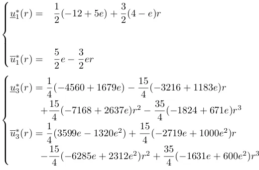
Example 6.3. Let u˜ = (er, e2−r). For m = 1 and m = 3, the best approximations of ˜u are u˜∗
1 and u˜∗3,
where:
u∗1(r) = 1
2(−12 + 5e) + 3
2(4−e)r
u∗1(r) =
5 2e−
3 2er
u∗3(r) = 1
4(−4560 + 1679e)− 15
4 (−3216 + 1183e)r +15
4 (−7168 + 2637e)r
2−35
4 (−1824 + 671e)r
3
u∗3(r) =
1
4(3599e−1320e
2) +15
4 (−2719e+ 1000e
2)r
−15
4 (−6285e+ 2312e
2)r2+35
4 (−1631e+ 600e
2)r3
and forq= 0.5 the distance (4.1)between u˜ andu˜∗
1 isD(˜u,u˜∗1) = 0.185451 and the distance betweenu˜ and
˜
u∗3 isD(˜u,u˜∗3) = 0.000835893.
Example 6.4. Letu˜= (ln [(e−1)r+ 1],2−ln [(e−1)r+ 1]),pi(r) =ri and an arbitraryq. The distances
(4.1)between u˜ andu˜∗m, form= 1,· · · ,7, are shown in Table 1.
m D(˜u,u˜∗m)
1 4.85342×10⁻²
2 7.2679×10⁻³
3 1.27813×10⁻³
4 2.44005×10⁻⁴
5 4.89405×10⁻⁵
6 1.04687×10⁻⁵
7 5.88816×10⁻⁶
Table 1: Distances for different values ofm
Regarding Theorem 5.1, it was predictable that increasing the variable m would reduce the associated
error. Since ˜uis a symmetric fuzzy number and by (4.38) the best approximation of it is independent ofq,
the distance (4.1) between ˜uand ˜u∗m is independent ofq.
Example 6.5. In this example, we approximate a fuzzy number withm= 1by a trapezoidal one and compare
the results from our method with the results obtained from other four methods proposed in [2,9,11,14] in a
u(r) /u(r) (1) (2) (3) (4) (5)
1−0.3√−lnr
2 + 0.7√−lnr
0.484391
1
2
3.20309
0.50052
0.96775
2.07526
3.16546
0.06790
1.67725
1.67725
3.2866
0.52195
0.89256
2.10743
2.9722
0.50052
0.96775
2.07526
3.16546
3r
7−3r
0.740495
3
4
6.2595
0.84003
2.80092
4.19908
6.15997
0.4905
3.5
3.5
6.5095
0.48633
2.97779
4.02221
6.51367
0.84003
2.80092
4.19908
6.15997
1 2 1 1 2 2 1 1 2 2
0.75
1.5
1.5
2.25
1 1 1 2 1 1 2 2
r+ 1
5−3r
1 2 2 5 1 2 2 5
−0.5
2
2
4.5
1
2
2
2.5
1
2
2
5
1
3−r
1 1 2 3 1 1 2 3
0.5
1.75
1.75
3
−0.33333
0.66667
2.33333
2.33333
1
1
2
3 Table 2. Numerical results of examples
As it is obvious, our method yields trapezoidal fuzzy numbers with closer cores in comparison with the
ones obtained from the other four methods. While the other four methods fail in approximating them-degree
polynomial form fuzzy numbers, our method can approximate all the trapezoidal, triangular andm-degree
polynomial form fuzzy numbers.
Example 6.6. Let u˜ = (2 +er−1,4−ln [(e−1)r+ 1]), pi(r) = ri. The distances between u˜ and u˜∗m, for
m= 0,· · · ,4 andq={0,0.25,0.5,0.75,1}, are shown in Table 3.
D(˜u,˜u∗m) q= 0 q= 0.25 q= 0.5 q= 0.75 q= 1
m= 0 0.504053 0.482261 0.459435 0.435415 0.409989
m= 1 0.0485342 0.0458563 0.0430119 0.0399657 0.0366673
m= 2 0.0072679 0.00643446 0.0054756 0.00430839 0.00267248
m= 3 0.00127813 0.00110962 0.000910436 0.000653097 0.000155493
This table shows that as the variablem increases, the distance (4.1) between exact given fuzzy number
and our approximated polynomial form fuzzy number reduces(it can be predicted by Theorem5.1). In this
example ˜uis not a symmetric fuzzy number. Hence, the distance between ˜uand ˜u∗
mdepends onq. As we can see in the table, wheneverqincreases from 0 to 1, the distance decreases. Considering the distance equation
(4.1), it can be deduced that the approximation of right spread is more precise than the approximation of
the left one.
7. Conclusion
In this paper, a new distance metric was proposed on the set of all fuzzy numbers with continuous left
and right spread functions. Using this metric, a given fuzzy number can be approximated through finding
the nearest polynomial form fuzzy number out of the set of allm-degree polynomial form fuzzy numbers.
Hence, two methods were proposed to solve the approximation problem. We showed that both of the
methods not only yield the same results, but also are convergent. Finally, we investigated our theorems in
some numerical examples.
References
[1] S. Abbasbandy, M. Amirfakhrian, The nearest trapezoidal form of a generalized left right fuzzy number,Int. J. Approx. Reason.43 (2006), 166-178.
[2] S. Abbasbandy, B. Asady, The nearest trapezoidal fuzzy number to a fuzzy quantity,Appl. Math. Comput.156 (2004), 381-386.
[3] M. Amirfakhrian, Numerical Solution of a System of Polynomial Parametric form Fuzzy Linear Equations, Book Chapter of Ferroelectrics, INTECH Publisher, Austria, (2010).
[4] A. I. Ban, L. Coroianu, Existence, uniqueness and continuity of trapezoidal approximations of fuzzy numbers under a general condition, Fuzzy Sets Syst. 3 (2014) 3-22.
[5] D. Dubois, H. Prade, Fuzzy Sets and Systems: Theory and Application, Academic Press, New York, (1980).
[6] L. Coroianu, M. Gagolewski, P. Grzegorzewski, Nearest piecewise linear approximation of fuzzy numbers,Fuzzy Sets Syst.
233 (2013), 26-51.
[7] P. Grzegorzewski, Metrics and orders in space of fuzzy numbers,Fuzzy Sets Syst. 97 (1998), 83-94. [8] P. Grzegorzewski, Nearest interval approximation of a fuzzy number,Fuzzy Sets Syst.130 (2002), 321-330. [9] P. Grzegorzewski, P. Mr´o wka, Trapezoidal approximations of fuzzy numbers,Fuzzy Sets Syst.153 (2005), 115-135. [10] P. Grzegorzewski, K. Pasternak-Winiarska,Natural trapezoidal approximations of fuzzy numbers, Fuzzy Sets Syst. 250
(2014), 90-109.
[11] M. Ma and A. Kandel and M. Friedman, Correction to ”A new approach for defuzzification”,Fuzzy Sets Syst.128 (2002), 133-134.
[12] V. Powers, B. Reznick, Polynomials that are positive on an interval, Trans. Amer. Math. Soc. 352 (10) (2000), 4677C4692. [13] J. Stolfi, M.V.A. Andrade, J.L.D. Comba, and R.Van Iwaarden. Affine arithmetic: a correlation-sensitive variant of interval
arithmetic, accessed January 17, (2008).