Volume 16, Number 6 (2018), 842-855
URL:https://doi.org/10.28924/2291-8639 DOI:10.28924/2291-8639-16-2018-842
NUMERICAL SOLUTION AND ANALYSIS FOR ACUTE AND CHRONIC HEPATITIS B
MUHAMMAD FARMAN, ZAFAR IQBAL, AQEEL AHMAD∗, ALI RAZA AND EHSAN
UL HAQ
Department of Mathematics and Statistics, The University of Lahore, Lahore, Pakistan.
∗Corresponding author: [email protected]
Abstract. In this article, we present the transmission dynamic of the acute and chronic hepatitis B epidemic problem to control the spread of hepatitis B in a community. In order to do this, first we present sensitivity analysis of the basic reproduction numberR0. We develop a unconditionally convergent nonstandard finite
difference scheme by applying Mickens approachφ(h) =h+O(h2) instead ofhto control the spread of this
infection, treatment and vaccination to minimize the number of acute infected, chronically infected with hepatitis B individuals and maximize the number of susceptible and recovered individuals. The stability analysis of the scheme has been developed by theorems which shows the both stable locally and globally. Comparison is also made with standard nonstandard finite difference scheme. Finally numerical simulations are also established to investigate the influence of the system parameter on the spread of the disease.
1. Introduction
The scope of mathematics includes mathematical modeling and esoteric mathematics. The flow of work,
process, predictions and outcomes can easily be measured with the help of mathematical concepts and theory.
Therefore, biologists are now extremely dependent on mathematics. Mathematical modeling of biological
sciences is done by many brilliant scientist [1-3]. The relationship between simple mathematical modeling
involves biological system, integer order differential equations that show their dynamics and complex system
Received 2018-06-26; accepted 2018-09-09; published 2018-11-02. 2010Mathematics Subject Classification. 37C75, 65L07.
Key words and phrases. sensitivity analysis; acute hepatitis B; chronic hepatitis B; NSFD.
c
2018 Authors retain the copyrights
of their papers, and all open access articles are distributed under the terms of the Creative Commons Attribution License.
which describes their changing of structure. The nonlinearity and multi-scale behaviors in mathematical
modeling describe the mutual relationship between parameter [4]. In last few decades, many biological
models were studied in detail by using classical derivative, few of them in [5,6].
Hepatitis B is a potentially life-threatening liver infection caused by the hepatitis B virus. It is a major
global health problem. It can cause chronic liver disease and chronic infection and puts people at high risk
of death from cirrhosis of the liver and liver cancer [7]. Infections of hepatitis B occur only if the virus is
able to enter the blood stream and reach the liver. Once in the liver, the virus reproduces and releases large
numbers of new viruses into the blood stream [8].
This infection has two possible phases: (1) acute and (2) chronic. Acute hepatitis B infection lasts less
than six months. If the disease is acute, your immune system is usually able to clear the virus from your
body, and you should recover completely within a few months. Most people who acquire hepatitis B as adults
have an acute infection. Chronic hepatitis B infection lasts six months or longer. Most infants infected with
HBV at birth and many children infected between 1 and 6 years of age become chronically infected [7].
About two-thirds of people with chronic HBV infection are chronic carriers. These people do not develop
symptoms, even though they harbor the virus and can transmit it to other people. The remaining one-third
develop active hepatitis, a disease of the liver that can be very serious. More than 240 million people have
chronic liver infections. About 600 000 people die every year due to the acute or chronic consequences of
hepatitis B [7,9]
HBV can be transmitted from one individual to another individual on different ways, such as transmission
of blood, semen and vaginal secretions [20,21,22]. Another major transmission of HBV is the unprotected
sexual contact, sharing of razors, blades or tooth brushes [3].Also the virus transmits from an infected
mother to her child during the time of birth. However, HBV cannot be transmitted through water, food,
hugging, kissing and causal contact such as in the work place, school, etc. [22]. The mode of transmission of
HBV and HIV is the same, but HBV is 50100 times more infectious [25]. HBV infection is a global health
problem. According to WHO about 400million population is infected world wide chronically. In China
93million population are affected due to HBV infections [23,27,28]. Vaccine for the prevention of hepatitis B
is available in the market that is very effective [24,26]. In the real world phenomena mathematical modeling
is one of the powerful tools to describe the dynamical behavior of different diseases [16,17,18,19,29].
Mathematical models have been used to help understand the dynamics of viral infections, such as human
immunodeficiency virus and hepatitis C infection [11,12]. Following these approaches, dynamic models were
developed to analyze the changes in hepatitis B virus levels during drug therapy [13,14,15,10]. In this
article,we develop a HBV transmission model. The infectious class is divided into two stages, such as acute
susceptible,I1(t) infected with acute hepatitis B,I2(t) infected with chronic hepatitis B andR(t) recovered
individuals.
In this paper, we investigate the stability and qualitative analysis of acute and chronic hepatitis B model.
An unconditionally convergent nonstandard finite difference scheme has been presented to obtain solution
of model. The analysis of two different states disease free and endemic equilibrium which means the disease
dies out or persist in a population has been made by finding reproductive number. Numerical results are
presented graphically to show the dynamics of the model.
2. Materials and Method
we used a mathematical model for HBV transmission by extending the work presented in [28].We divide the
host population denoted by T(t) into four compartments: susceptible individualsS(t), who are not infective
but have the chance to catch the disease; infected I1(t) represents those individuals who are infective with
acute hepatitis; I2(t) are those individuals, who are infected with chronic hepatitis and R(t) represents
those individuals who have recovered after the infection with a life-time immunity. The flowchart for the
transmission of HBV is given in Figure 1.
Figure 1. The flowchart of the model
Thus, the mathematical model is represented by the following four differentials equations:
dS
dt =b−αS(t)I2(t)−(µ0+ν)S(t) (2.1)
dI1
dI2
dt =βI1(t)−(µ0+µ1+γ2)I2(t) (2.3)
dR
dt =γ1I1(t) +γ2I2(t) +νS(t)−µ0R(t) (2.4)
with initial conditions S(0)≥0, I1(0)≥0, I2(0)≥, R(0) ≥0, Hereb represents the birth rate, αis the
moving rate from susceptible to infected with acute hepatitis B, β is the moving rate from acute stage to
infected with chronic hepatitis, γ1 is the recovery rate from acute stage to recovered, γ2 is the recovery
rate from chronic stage to recovered compartment, µ0 is the death rate occurring naturally, which is also
called natural mortality rate,µ1 is the death rate occurring due to hepatitis B andν represents hepatitis B
vaccination rate.
3. Qualitative Analysis
The model (2.1−2.4) is locally asymptotically as well as globally asymptotically stable at disease-free
and endemic equilibrium points [29]. For disease-free equilibrium the model (2.1−2.4) is both locally and
globally stable, if the value of basic reproduction number is less than unity while for the endemic equilibrium
the model is stable if the value of the basic reproduction number R0 is greater than unity. Model has a
disease-free equilibrium, denoted byE0 and defined as,E0= (S0,0,0, R0), where
S0= b µ0+ν
and
R0= νb
µ0(µ0+ν) .
The endemic equilibrium is given byE∗= (S∗, I1∗, I2∗, R∗), where
S∗= 1
αβ(µ0+β+γ1)(µ0+µ1+γ2)
I1∗= 1
αβ(µ0+ν)(µ0+µ1+γ2)[R0−1]
I2∗= 1
α(µ0+ν)[R0−1]
R∗= 1
µ0 [(γ1
αβ(µ0+ν)(µ0+µ1+γ2) + γ2
α(µ0+ν)[R0−1]) + ν
αβ(µ0+β+γ1)(µ0+µ1+γ2)]
Regarding these equilibrium point of the model (2.1−2.4), we have the following results which are proved
3.1. Reproductive Number. Basic reproduction number R0 is defined to be the expected number of
secondary infections produced by an index case or the average number of secondary infection arising from a
single individual introduced into the susceptible class during its entire infectious period in a totally susceptible
population. The basic reproduction numberR0 of the model (2.1−2.4) in [29] is
R0=
αβb
(µ0+ν)(µ0+β+γ1)(µ0+µ1+γ2)
Theorem 3.1. IfR0<1, then the model(2.1−2.4)is locally asymptotically stable at disease-free equilibrium,
E0= (µb
0+ν,0,0,
νb
µ0(µ0+ν)), whileE0 is unstable saddle point ifR0>1.
Theorem 3.2. If R0≤1, then the model(2.1−2.4)is globally asymptotically stable at disease-free
equilib-rium,E0= (S0,0,0, R0)and unstable otherwise.
Theorem 3.3. The endemic equilibrium state E1 = (S∗, I1∗, I2∗, R∗) of the model (2.1−2.4) is globally
asymptotically stable, ifR0>1, otherwise unstable.
Prof of these theorems will be given in [29], used in section 4.
3.2. Sensitivity Analysis of R0: The sensitivity of
R0=
αβb
(µ0+ν)(µ0+β+γ1)(µ0+µ1+γ2)
to each of its parameters is
∂R0 ∂α =
βb
(µ0+ν)(µ0+β+γ1)(µ0+µ1+γ2) ≥0
∂R0 ∂β =
αb(µ0+γ1)
(µ0+ν)(µ0+β+γ1)2(µ0+µ1+γ2) ≥0
∂R0 ∂b =
αβ
(µ0+ν)(µ0+β+γ1)(µ0+µ1+γ2) ≥0
∂R0 ∂ν =−
αβb
(µ0+ν)2(µ0+β+γ1)(µ0+µ1+γ2) ≤0
∂R0 ∂γ1
=− αβb
(µ0+ν)(µ0+β+γ1)2(µ0+µ1+γ2) ≤0
∂R0 ∂γ2
=− αβb
(µ0+ν)(µ0+β+γ1)(µ0+µ1+γ2)2 ≤0
∂R0 ∂µ1
=− αβb
(µ0+ν)(µ0+β+γ1)(µ0+µ1+γ2)2 ≤0
∂R0 ∂µ0
=−αβb[(µ0+ν)(µ0+β+γ1) + (µ0+ν)(µ0+µ1+γ2) + (µ0+β+γ1)(µ0+µ1+γ2)] (µ0+ν)2(µ0+β+γ1)2(µ0+µ1+γ2)2
≤0
It can be seen thatR0 is most sensitive to change in parameter, here,R0is increasing withα, b, β,and
decreasing withγ1, γ2, ν, µ0, µ1. In other words it found that the sensitivity analysis shows that prevention
4. Nonstandard Finite Difference (NSFD) Scheme
A nonstandard finite difference (NSFD) scheme for the system (2.1−2.4) is presented in this section [30].
In recent years, nonstandard finite difference (NSFD) scheme for discrete models have been constructed or
tested for a wide range of nonlinear systems of differential equations [31,32,33]. The positivity of the state
variables involved in the system is satisfy by proposed method. This property has key role when we solve
mathematical models arising in biology because these state variables represent sub-populations which never
take negative values. The discretized form of the the system (2.1−2.4) by using NSFD scheme which based
on the generalized first order forward method is written as
Sk+1−Sk
h =b−αs k+1Ik
2 −(µ0+ν)Sk+1 (4.1)
Sk+1+hαsk+1I2k+h(µ0+ν)Sk+1=Sk+bh (4.2)
Sk+1= S
k+bh
1 +hαIk
2 +h(µ0+ν)
(4.3)
I1k+1−I1k h =αI
k
2Sk+1−(β+µ0+γ1)I1k+1 (4.4)
I1k+1+h(β+µ0+γ1)I1k+1=I k 1 +hαI
k 2S
k+1 (4.5)
I1k+1= I k
1 +hαI2kSk+1 1 +h(β+µ0+γ1)
(4.6)
I2k+1−Ik 2 h =βI
k+1
1 −(µ1+µ0+γ2)I2k+1 (4.7)
I2k+1+h(µ1+µ0+γ2)I2k+1=I k 2+hβI
k+1
1 (4.8)
I2k+1= I k 2 +hβI
k+1 1 1 +h(µ1+µ0+γ2)
(4.9)
Rk+1−Rk h =γ1I
k+1
1 +γ2I2k+1+νS k+1−µ
0Rk+1 (4.10)
Rk+1(1 +hµ0) =Rk+h(γ1I1k+1+γ2I2k+1+νS
k+1) (4.11)
Rk+1= R k+h(γ
1I1k+1+γ2I2k+1+νSk+1) 1 +hµ0
4.1. Proposed NSFD Scheme. In this section, we design an NSFD scheme [34] that replicates the
dy-namics of the continuous model (2.1−2.4). LetYk = (Sk, I1k, I2k, Rk)T denoted an approximation ofX(tk)
wheretk=k∆t, withk∈ N,h= ∆t >0 be a step size then
Sk+1−Sk
φ =b−αs k+1Ik
2 −(µ0+ν)Sk+1 (4.13)
I1k+1−Ik 1 φ =αI
k 2S
k+1−(β+µ
0+γ1)I1k+1 (4.14)
I2k+1−I2k φ =βI
k+1
1 −(µ1+µ0+γ2)I2k+1 (4.15)
Rk+1−Rk φ =γ1I
k+1
1 +γ2I2k+1+νS k+1−µ
0Rk+1 (4.16)
which is the new purposed NSFD scheme for the given model, where
φ=φ(h) = 1−e
−(β+µ0+γ1)h
β+µ0+γ1
(4.17)
The discrete method (4.13−4.16) is indeed an NSFD scheme because it is constructed according to
Mickens rules [33] formalized as follows in [34].
Rule 1. The standard denominatorh= ∆tof the discrete derivatives is replaced by the complex denominator
function in Equation (4.17) which satisfies the asymptotic relation
φ(h) =h+O(h2)
Note that the denominator functionφis expected to better capture the dynamics of the continuous model
through the presence of the underlying parameters µ0, β, γ1. In fact, exact schemes for a wide range of
dynamical systems involve such complex denominator functions [35,36].
Rule 2.Nonlinear terms in the right-hand side of Equation (2.1−2.4) are approximated in a non-local way.
For instance, we haveI2(tk)S(tk)'I2kSk+1 instead ofI2(tk)S(tk)'I2kSk
4.2. Analysis of the Scheme.
Theorem 4.1. The NSFD scheme (4.13−4.16)is a dynamical system on the biological feasible domainK
of the continuous model(2.1−2.4).
Proof:First, we prove the positivity of the scheme (4.13−4.16). It is easy to show that the NSFD scheme
(4.13−4.16)takes the explicit form
Sk+1= S
k+φb
1 +αφIk
I1k+1= [1 +αφI k
2 + (µ0+ν)φ][I1k+αφ(Sk+φb)I2k] [1 +φ(µ0+β+γ1)][1 +αφI2k+ (µ0+ν)φ]
I2k+1=[1 +φ(µ0+β+γ1)][1 +αφI k
2+ (µ0+ν)φ](I2k+βφI1k) +βαφ2(Sk+φb)I2k [1 +φ(µ0+µ1+γ2)][1 +φ(µ0+β+γ1)][1 +αφI2k+ (µ0+ν)φ]
Rk+1= R
k.A.B.C.D+φ{γ
1(A.D.CI1k+αφ.E) +γ2A(B.C[I2k+βφI1k] +αβφ2I2k.E) +νE.A.B.C} A.B.C.D
where
A= 1 +µ0φ, B= 1 +φ(µ0+β+γ1), C= 1 +αφI2k+ (µ0+ν)φ
D= 1 +φ(µ0+µ1+γ2), E=Sk+φb
Thus Sk+1 ≥0, Ik+1
1 ≥ 0, I k+1
2 ≥ 0, Rk+1 ≥ 0 whenever the discrete variables are non-negative at the
previous iteration. It remains to prove the positive invariance ofK. Adding the (4.13)and(4.14),we have
[1 +φ(µ0+ν)]Hk+1=φb+Hk−[1 + (µ0+µ1+γ1)φ]Ik ≤φb+Hk
[1 +φ(µ0+ν)]Hk+1≤φb+Hk
⇒Hk+1≤ b µ0+ν
whenever
Hk ≤ b µ0+ν
The priori bonds for I2k+1 and Rk+1 follow the radially from the fact that Ik+1 2 andI
k+1
1 and less then or
equal Hk+1. This complete the proof.
Theorem 4.2. (1) The disease-free fixed point (resp. the endemic fixed point ) of the NSFD scheme(4.13−
4.16) for the model without recruitment/provision of disease is GAS whenever R0 ≤ 1 (resp. whenever
R0>1).
(2) The endemic fixed-point of the NSFD scheme(4.13−4.16)for the full model is GAS.
Proof:Let Yk ∈ R4+ be the bounded sequence defined by the NSFD scheme (4.13−4.16). We want to prove
that Yk tends to Y∗, where Y∗ is any of the fixed point. By Bolzano Weierstrass theorem, there exists a
subsequence Ynk of Yn that converge to some Z
∗ as k → +∞. By the assumption made above and the
E0(wheneverR0≤1)or the unique endemic fixed-pointE∗ or the unique endemicE, which is LAS thanks
to Theorem 4.2. Therefore, there exists θ >0 such that for an initial conditionY0 satisfying
kY0−Y∗k ≤θ
we have
lim x→+∞kY
0−Y∗k= 0 (4.18)
letY0 be an arbitrary initial condition . As
lim
x→+∞Ynk=Y
∗,
there exits a integerk0 such that
kYnk0−Y
∗k ≤θ (4.19)
In view equation (4.18)and(4.19), we have
lim
x→+∞,n≥1kYnn−Y
∗k= lim
x→+∞,n≥nk0
kYnn−Y
∗k= 0 (4.20)
This prove that Y∗ is GAS.
Table 1. Values of physical parameters used in model whenR0<1
Parameter Value Parameter Value
n1 100 n2 40
n3 20 n4 5
b 0.4 ν 0.02
β 0.01 µ0 0.03
µ1 0.002 γ1 0.05
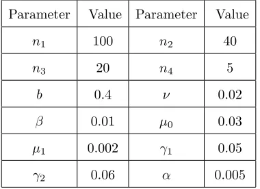
Table 2. Values of physical parameters used in model whenR0>1
Parameter Value Parameter Value
n1 100 n2 40
n3 20 n4 5
b 0.4 ν 0.02
β 0.1 µ0 0.03
µ1 0.04 γ1 0.05
γ2 0.06 α 0.05
4.3. Numerical Simulations. The mathematical analysis of epidemic model hepatitis B with non-linear
incidence has been presented. To observe the effects of the parameters using in this dynamics hepatitis B
model (2.1−2.4), conclude several numerical simulations varying the value of parameters given in table 1 and
table 2 forR0<1 andR0>1 respectively. Figure 2 and 3 shows the convergence solution for diseases free
and endemic equilibria by using NSFD scheme ath= 1. Figure 4 and 5 also represent the he convergence
solution for diseases free and endemic equilibria by using NSFD scheme atφ=φ(h) +O(h2). The technique
create a better impact to control the hepatitis B, it reduces the infected rate and increases the susceptible
and recovered population during disease free state as well as in endemic state.
0 50 100 150 200 250 300
0 10 20 30 40 50 60 70 80 90 100
Disease Free Equilibrium
Time,Step size h=1
Comparmental Population
Susceptible
Infected with Acute HB Infected with Chronic HB Recovered
Figure 2. Numerical solutions for susceptible, acute infected individual, chronic infected
individual and recovered population in a timetwith step sizeh= 1 for disease free
0 50 100 150 200 250 300 0
10 20 30 40 50 60 70 80 90 100
Endemic Equilibrium
Time,Step size h=1
Comparmental Population
Susceptible
Infected with Acute HB Infected with Chronic HB Recovered
Figure 3. Numerical solutions for susceptible, acute infected individual, chronic infected
individual and recovered population in a timetwith step sizeh= 1 for endemic equilibrium
points.
0 50 100 150 200 250 300
0 10 20 30 40 50 60 70 80 90 100
Disease Free Equilibrium
Time
Comparmental Population
Susceptible
Infected with Acute HB Infected with Chronic HB Recovered
Figure 4. Numerical solutions for susceptible, acute infected individual, chronic infected
individual and recovered population in a timet by usingφ=φ(h) with step size h= 1 for
0 50 100 150 200 250 300 0
10 20 30 40 50 60 70 80 90 100
Endemic Equilibrium
Time
Comparmental Population
Susceptible
Infected with Acute HB Infected with Chronic HB Recovered
Figure 5. Numerical solutions for susceptible, acute infected individual, chronic infected
individual and recovered population in a timet by usingφ=φ(h) with step size h= 1 for
endemic equilibrium points.
5. Conclusion
We have considered a mathematical system of equation which describes the hepatitis B disease. The
analysis of the system is well established. Sufficient conditions for local stability of the DFE point E0
are given in terms of the basic reproduction number R0 of the model, where it is asymptotically stable if
R0 < 1. The positive infected equilibrium E∗ exist when R0 >1 and sufficient conditions that guarantee
the asymptotic stability of the point are given. Beside this sensitivity analysis of the parameters involved
in threshold parameter R0 is discussed. It is important to note that nonstandard finite difference scheme
for mathematical models based on system of differential equations is more powerful approach to compute
the convergent solutions for the disease models. The nonstandard finite difference scheme is dynamically
consistent, easy to implement and show a good agreement to control the bad impact of hepatitis B for
long period of time and to eradicate a death killer factor in the world spread by hepatitis B. Finally, we
presented the numerical simulation and verified all the analytical results numerically by using nonstandard
finite difference scheme to reduce acute as well chronic infected rates for both disease free and endemic
equilibria , we are able to control the spreading of hepatitis B in the community.
References
[2] S. Busenberg, P. Driessche, Analysis of a disease transmission model in a population with varying size, J. Math. Biol. 28 (1990), 65-82.
[3] A.M.A. El-Sayed, S.Z. Rida and A.A.M. Arafa, On the solutions of time-fractional bacterial chemotaxis in a diffusion gradient chamber, Int. J. Nonlinear Sci. 7 (2009), 485-495.
[4] O.D. Makinde, Adomian decomposition approach to a SIR epidemic model with constant vaccination strategy, Appl. Math. Comput. 184 (2007), 842-848.
[5] A.A.M. Arafa, S.Z. Rida and M. Khalil, Fractional modeling dynamics of HIV and 4 T-cells during primary infection, Nonlinear Biomed. Phys. 6 (2012), 1-7.
[6] C.M. Kribs-Zaleta, Structured models for heterosexual disease transmission, Math. Biosci. 160 (1999), 83-108.
[7] B. Buonomo and D. Lacitignola, On the dynamics of an SEIR epidemic model with a convex incidence rate, Ricerche Mat. 57 (2008), 261-281.
[8] WHO, Hepatitis B Fact Sheet No. 204, The World Health Organisation, Geneva, Switzerland, 2013, http://www.who.int/mediacentre/factsheets/fs204/en/.
[9] Canadian Centre for Occupational Health and Safety, Hepatitis B,http://www.ccohs.ca/oshanswers/diseases/hepatitisb.html.
[10] A. V. Kamyad, R. Akbari, A. K Heydari and A. Heydari Mathematical Modeling of Transmission Dynamics and Optimal Control of Vaccination and Treatment for Hepatitis B Virus, Comput. Math. Methods Med. 2014 (2014), Article ID 475451. [11] C.M. Stanca, R.M. Ruy, W.N. Patrick and S.P. Alan, Modeling the mechanisms of acute hepatitis B virus infection, J.
Theor. Biol. 247 (2007), 23-35.
[12] A. Perelson, Modelling viral and immune system dynamics. Nature Rev. Immunol. 2 (2002), 28-36.
[13] A. Perelson and R. Ribeiro, Hepatitis B virus kinetics and mathematical modeling. Sem. Liv. Dis. 24 (2004), 11-15. [14] M. Nowak, S. Bonhoeffer,A. Hill, R. Boehme, H. Thomas, H. McDade, Viral dynamics in hepatitis B infection. Proc. Natl
Acad. Sci. USA 93 (1996), 4398-4402.
[15] S. Lewin, R. Ribeiro, T. Walters, G. Lau, S. Bowden, S. Locarnini and A. Perelson, Analysis of hepatitis B viral load decline under potent therapy: complex decay profiles observed. Hepatology 34 (2001), 1012-1020.
[16] P. Colombatto, L. Civitano, R. Bizzarri, F. Oliveri, S. Choudhury, R. Gieschke, F. Bonino and M.R. Brunetto, A multiphase model of the dynamics of HBV infection in HBeAg-negative patients during pegylated interferon-a2a, lamivudine and combination therapy. Antiviral Therapy 11 (2006), 197-212.
[17] J. Wang, J. Pang and X. Liu,Modelling diseases with relapse and nonlinear incidence of infection: A multi-group epidemic model, J. Biol. Dyn. 8 (2014), 99-116.
[18] J. Wang, R. Zhang and T. Kuniya, The stability analysis of an SVEIR model with continuous age-structure in the exposed and infectious classes, J. Biol. Dyn. 9 (2015), 73-101.
[19] G. Zaman, Y.H. Kang and I.H. Jung, Stability and optimal vaccination of an SIR Epidemic Model, BioSystems 93 (2008), 240249.
[20] G. Zaman, Y.H. Kang and I.H. Jung, Optimal treatment of an SIR epidemic model with time delay, BioSystems 98 (2009), 43-50.
[21] D. Lavanchy, Hepatitis B virus epidemiology, disease burden, treatment, and current and emerging prevention and control measures, J. Viral Hepat. 11 (2004), 97-107.
[22] A.S. Lok, E.J Heathcote and J.H. Hoofnagle, Management of hepatitis B, 2000 Summary of a workshop, Gastroenterology 120 (2001), 18281853.
[24] M.K. Libbus and L.M. phillips, Public health management of perinatal hepatitis B virus, Public Health Nurs. 26 (2009), 353-361.
[25] J.E. Maynard, M.A. Kane and S.C. Hadler, Global control of hepatitis B through vaccination role of hepatitis B vaccine in the expanded programme on immunization, Rev. Infect. 2 (1989), S574-S578.
[26] S. Thornley, C. Bullen and M. Roberts,Hepatitis B in a high prevalence NewZealand population: A mathematical model applied to infection control policy, J. Theor. Biol. 254 (2008), 599-603.
[27] C.W. Shepard, E.P. Simard, L. Finelli, A.E. Fiore and B.P. Bell, Hepatitis B virus infection epidemiology and vaccination, Epidemiol. Rev. 28 (2006), 112-125.
[28] R. Williams, Global challenges in liver disease, Hepatology 44 (2006), 521-526.
[29] T. Khan, G. Zaman and M. I. Chohan, The transmission dynamic and optimal control of acute and chronic hepatitis B, J. Biol. Dyn. 11(2017), 172-189.
[30] R. E. Mickens, Exact solutions to a finite difference model of a nonlinear reactions advection equation: Implications for numerical analysis, Numer. Methods Partial Differ. Equ. 5 (1989), 313-325.
[31] R. E. Mickens, Applications of Nonstandard finite difference Schemes, World Scientific, Singapore (2000).
[32] R. Anguelov and J.M.S Lubuma, Nonstandard finite difference method by nonlocal approximations, Math. Comput. Simul. 61 (2003), 465-475.
[33] R.E. Mickens, Nonstandard finite difference Models of differential equations, World Scientific, Singapore (1994).
[34] R. Anguelov and J.M.S. Lubuma, Contributions to the mathematics of the nonstandard finite differencemethodandappli-cations, Numer. Methods Partial Differ. Equ. 17 (2001), 518-543.
[35] J.M.S. Lubuma and K.C. Patidar, Non-standard methods for singularly perturbed problems possessing oscillatory/layer solutions, Appl. Math. Comput. 187(2) (2007), 1147-1160.