R E S E A R C H
Open Access
Exploiting bounded signal flow for graph
orientation based on cause
–
effect pairs
Britta Dorn
1, Falk Hüffner
2*, Dominikus Krüger
3, Rolf Niedermeier
2and Johannes Uhlmann
2Abstract
Background:We consider the following problem: Given an undirected network and a set of sender–receiver pairs, direct all edges such that the maximum number of“signal flows” defined by the pairs can be routed respecting edge directions. This problem has applications in understanding protein interaction based cell regulation mechanisms. Since this problem is NP-hard, research so far concentrated on polynomial-time approximation algorithms and tractable special cases.
Results:We take the viewpoint of parameterized algorithmics and examine several parameters related to the maximum signal flow over vertices or edges. We provide several fixed-parameter tractability results, and in one case a sharp complexity dichotomy between a linear-time solvable case and a slightly more general NP-hard case. We examine the value of these parameters for several real-world network instances.
Conclusions:Several biologically relevant special cases of the NP-hard problem can be solved to optimality. In this way, parameterized analysis yields both deeper insight into the computational complexity and practical solving strategies.
Background
Current technologies [1] like two-hybrid screening can find protein interactions, leading to protein-protein interaction (PPI) networks, but cannot decide the direc-tion of the interacdirec-tion. This can be complemented by gene knock-out experiments which constitute a way to determine causal relations in these networks, thus pro-viding additional information on possible directions of information flow in them [2]. Given a list of so-called cause–effect pairs, the challenge consists in deducing an orientation of the PPI network which takes into account the causal relations of as many of these pairs as possible. Medvedovsky et al. [3] formalize this in terms of a graph theoretical problem as follows.
Problem Formalization
Let G= (V,E) be an undirected graph. An orientationG ofGis a directed graphG = (V,E) obtained from Gby replacing every undirected edge {u, v}Î Eby a directed one, i. e., either by (u,v)Î Eor by (v, u)ÎE. LetP⊆V
×V be a set of ordered source–target pairs, which we sometimes refer to as “signals”. In order to distinguish pairs from edges or arcs, we use the notation [a, b]Î P to denote the pair starting inaand ending inb. We say that a pair [a,b]Î Pissatisfiedby a given orientation
G if there exists a directed path fromatob inG. The central problem considered in this work is to find an orientation of a given graph maximizing the number of satisfied pairs. As pointed out by Medvedovsky et al. [3], we can assume that the given graph is a tree: it is clearly optimal to orient the edges of a cycle to form a directed cycle, and hence one can repeatedly contract a cycle to a single vertex, obtaining a tree. Note that this process will always produce the same tree independent of the order of contractions, since two vertices will be merged eventually if and only if they are in the same bridge block, where a bridge block is a connected component of the graph that is obtained by deleting all bridges (edges whose deletion increases the number of con-nected components). Further, bridge blocks can be found in linear time [4,5]. Thus, formalized as a decision problem, MAXIMUM TREE ORIENTATION is defined as follows.
* Correspondence: [email protected] 2
Institut für Softwaretechnik und Theoretische Informatik, TU Berlin, Berlin, Germany
Full list of author information is available at the end of the article
Maximum Tree Orientation (MTO)
Input: An undirected tree T, a setP of ordered pairs of vertices ofT, and an integerk≥0.
Question: Is there an orientation ofTsuch that at most kpairs inPare not satisfied?
We also consider the weighted version, called WEIGHTEDMAXIMUMTREEORIENTATION(W-MTO), where every pair [a,b]Î Pis associated with a rational weight
ω([a, b]) ≥0, and the goal is to maximize the sum of weights of the satisfied pairs. Throughout this work, n denotes the number of vertices in the given MTO instance, if not stated otherwise.
As sketched before, MTO is motivated from the infer-ence of causal relations in biological networks [6,7] such as PPI networks, but it also has applications in the con-text of communication networks, where several one-way connection request pairs are given. Since each link between two network nodes can only be used in one direction, one has to orient the links in such a way that as many communication requests as possible can be fulfilled.
Previous Work
MTO was introduced by Medvedovsky et al. [3]; they showed that the problem is NP-complete even when the underlying tree is a star (that is, a diameter-two tree) or a tree with maximum vertex degree three. Moreover, they provided a cubic-time algorithm for MTO restricted to paths. Seeing MTO as the task to maximize the number of satisfied pairs, Medvedovsky et al. also provided polynomial-time approximation algorithms with approximation factor 1/4 in the case of stars andO(1/log n) in the case of general n-vertex trees. The latter approximation factor was recently improved to O(log log n/log n) by Gamzu et al. [8], who furthermore extended the studies of MTO to
“mixed graphs” where some of the edges are already oriented based on causal relations known in advance. Besides these theoretical investigations, Medvedovsky et al. [3] also provided some experimental results based on a yeast PPI network and some synthetic data. Silverbush et al. [9] recently formulated a polynomial-size integer linear program for the generalization of mixed graphs and did some experiments with it. Also recently, Gitter et al. [10] considered graph orientation with the objective of maximizing the weight of all satisfied paths between sources and targets with length at most some constant k. They used approximation algorithms to discover pathways in biological networks. In an earlier work, Hakimi et al. [11] studied the spe-cial case of MTO where the list of pairs to be satisfied containsall possible pairs; they developed a quadratic-time algorithm for this case.
Our Contributions
We mainly continue and complement previous work on MTO [3,8] by starting a parameterized and multivariate complexity analysis of MTO. That is, we try to better understand the border between tractable and intractable cases of MTO while sticking to optimal (instead of approximate) solutions. In particular, our focus is on the
“amount of signal flow” over vertices and edges, respec-tively, and how this influences the computational com-plexity of MTO.
• We show that W-MTO can be solved in
O(2mv· |P|+n4)time on an n-vertex tree, where m v denotes the maximum number of connecting paths (one-to-one corresponding to the input vertex pairs) over any tree vertex. In other words, W-MTO is fixed-parameter tractable with respect to the fixed-parametermv.
•We introduce the concept of cross pairs and show that cross-pair-free instances of W-MTO can be solved in quadratic time, as a corollary also improving the cubic-time algorithm of Medvedovsky et al. [3] for MTO on paths to quadratic time.
• We additionally show that W-MTO is fixed-para-meter tractable with respect to the parafixed-para-meter qv which is the maximum number of cross pairs over any vertex; namely, it can be solved inO(2qv·n2·q
v)time.
• Shifting the focus from “maximum vertex signal flow”to“maximum edge signal flow”, we show a sharp complexity dichotomy: W-MTO can be solved in linear time if no tree edge has to carry more than two signals, but if this maximum edge signal flow is three, MTO already becomes NP-hard.
•Finally, we briefly discuss some practical aspects of exactly solving the so far very few considered real-world instances and conclude that these can be already solved to optimality within milliseconds (via at least three dif-ferent strategies). However, we also make the point that with the future availability of further real-world data, our new algorithms could be of significant practical rele-vance beyond so far known or straightforward approaches.
Preliminaries, Basic Facts, and Simple Observations
For ease of presentation, for a W-MTO instance (T,P,
b, or talk about pairs and paths interchangeably. Some-times, we also talk about paths in the tree which do not necessarily correspond to pairs. We denote the undir-ected path connecting verticesvandwin Tby pathT(v, w). Moreover, Pv:= {[s, t] Î P | v ÎV (pathT(s, t))} denotes the set of pathspassing through a vertex v(note that this includes paths of which vis an endpoint). An MTO instance is calledrootedif the underlying treeTis rooted. In a rooted tree T= (V,E), if vertexaÎVis an ancestor of vertexb ÎV, then we use the notation a≺ b. The subtree ofTrooted atvÎVis denoted Tv.
Let (T= (V,E),P) be an MTO instance, and letx,yÎ P be two pairs. We say that x conflicts with y if there exists no orientation of T for which both x and y are satisfied. From ann-vertex MTO instance, we build a so calledconflict graph in which each vertex corresponds to an input pair of the MTO instance, and where there is an edge between two pairs if and only if they conflict with each other. More formally, given an MTO instance (T = (V, E), P), the corresponding conflict graph Gc(T, P) is defined Gc(T,P) := (P,Ec) whereEc := {{u, v} |u,v ÎP∧uconflicts withv}.
The computation of the conflict graph can be done in Θ(n4) time. It clearly cannot be done faster, because up to O(n4) conflicts are possible. To achieve the desired bound, we thus need to decide in constant time whether two pairs conflict with each other. This is done using an appropriate data structure and two simple observations: First, in a rooted tree, least common ancestors (LCAs) can be calcu-lated in constant time after some linear time preprocessing [12]. Second, two pairs are in conflict if and only if their paths run in different directions through an edge incident on the lower one of the two LCAs of the two pairs. Clearly, for an orientation of (T,P), inGc there are no edges (that is, conflicts) between the vertices correspond-ing to the satisfied source–target pairs, and hence the ver-tices corresponding to the non-satisfied source–target pairs form a vertex cover forGc, that is, a vertex setV’⊆P such that for every edgeeÎEcat least one endpoint ofe is inV’. This yields the following useful observation.
Proposition 1. Finding a minimum-weight vertex cover in the conflict graph Gc(T, P) one-to-one corre-sponds to determining a minimum-weight set of pairs that cannot be satisfied in(T,P).
It is generally assumed that the fact that a problem is NP-hard implies that there is no algorithm that finds an optimal solution and has running time bounded by a polynomial of the size of the input. Parameterized com-plexity is a two-dimensionalframework for the analysis of computational complexity [13-15]. One dimension is the input size n, and the other one is theparameter (usually a positive integer). A problem is called fixed-parameter tractable (fpt) with respect to a parameterx if it can be solved in f(x) ⋅ nO(1) time, where f is a
computable function only depending onx. If a problem is fixed-parameter tractable with respect tox, we can hope for efficient optimal solutions as long as the para-meter is not too large. Due to Proposition 1 we can immediately conclude that MTO and W-MTO are fixed-parameter tractable with respect to the parameter
“number of pairs” p, since the conflict graph hasp ver-tices and we can find a minimum-weight vertex cover by trying all possibilities in 2p⋅nO(1)time. Further, since minimum-weight vertex covers can be found inO(1.379k + kn) time [16], we have fixed-parameter tractability with respect to the parameter “number of unsatisfied pairs”, and if all weights are at least one, also with respect to the parameter “total weight of unsatisfied pairs”.
Tree-decomposition-based algorithms have been suc-cessfully applied in the area of computational biology, for instance, in the context of structure–sequence align-ment [17]. Informally speaking, thetreewidth[15] mea-sures the “tree-likeness” of a graph, and a tree decomposition is the“embedding”of a graph into a tree depicting the tree-like structure of the graph.
We recall the following definitions from literature [18]: A tree decomposition of a graphG = (V, E) is a pair{Xi|i∈I},T, where each Xi is a subset ofVcalled bag, andT = (I,F)is a tree with node setIand edge set F. The following must hold:
1.i∈IXi=V;
2. for every edge {u,v}Î E, there is aniÎIsuch that {u,v}⊆Xi; and
3. for alli, j, lÎI, ifjlies on the path betweeniand l in T, thenXi∩Xl⊆Xj.
Thewidthof{Xi|i∈I},T, is max{|Xi| |iÎ I} - 1. The
treewidth of G is the minimum width over all tree
decompositions ofG.
Methods and Results
Bounded Signal Flow Over Vertices
Then, for a rooted MTO instance a cross pair is a source–target pair such that none of its endpoints is the ancestor of the other endpoint. By refining the solving strategy for cross-pair-free instances, we show that MAX-IMUMTREE ORIENTATION can be solved inO(2qv·n2·q
v)
time, whereqvdenotes the maximum number of cross pairs passing through a vertex.
All algorithms in this subsection are based on dynamic programming, and, hence, since source–target pair weights can easily be incorporated, extend to W-MTO.
Parameter“Maximum Number of Pairs Per Vertex”
Here, we show that W-MTO is fixed-parameter tract-able for the parametermvdenoting the maximum num-ber of source–target pairs passing through a vertex. To this end, we prove in Theorem 1 that we can construct in polynomial time a tree decomposition of the conflict graph of treewidth at most mv. Recall that (weighted) MTO is equivalent to (weighted) VERTEX COVERon the conflict graph (see Proposition 1). Thus, the running time follows by the fact that (weighted) VERTEX COVER can be solved in O(2twn) time, given a tree decomposi-tion of width tw [15]. □
Theorem 1. On n-vertex trees, WEIGHTED MAXIMUM TREE ORIENTATION is solvable inO(2mv· |P|+n4)time,
where mvdenotes the maximum number of source–target
pairs passing through a vertex.
Proof. First, we show how to construct a tree decom-position of widthmvof the conflict graph in polynomial time. Let (T= (V,E),P) denote an MTO instance and letGc= (P,Ec) denote the associated conflict graph. The basic idea is that we can useT as the underlying tree of a tree decomposition of Gc = (P,Ec). More specifically, the tree decomposition is given by〈{Pv| vÎV}, T〉for all vÎV. Recall that Pvdenotes the set of source–target pairs passing throughv. Observe that each vertexpÎPof the conflict graph appears exactly in the bagsXvfor all vÎV(pathT(p)). Moreover, note that if two source–target pairsp= [s,t] andp’= [s’,t’] are in conflict (and hence are adjacent in the conflict graph), then pathT(s,t) and pathT(s’,t’) have at least one edge and thus at least two vertices in common. Hence, every edge of the conflict graph is contained in at least one of theXv’s. Thus, all con-ditions of a tree decomposition are fulfilled. Moreover, the width of this tree decomposition is clearlymv- 1. The conflict graph, the setsPv, and the tree decomposition can be computed inO(n4) time. Thus, the overall running time follows by the fact that WEIGHTEDVERTEXCOVERcan be solved inO(2tw|P|) time, given a tree decomposition of width tw ofGc[15].
Cross Pairs
In Theorem 1, we have shown that W-MTO is fixed-parameter tractable with respect to the fixed-parametermv. In
the following, we will strengthen this result by showing that W-MTO is fixed-parameter tractable with respect to the parameter “number of a special type of source– target pairs (the so-called cross pairs) passing through a vertex”. The idea is to identify a“trivial”(that is, polyno-mial-time solvable) special case of the problem and then to investigate instances that are close to these trivial instances, their closeness measured in terms of a certain parameter which is referred to asdistance from triviality [19,20].
In the following, we will always considerrootedtrees. Informally speaking, a cross-pair-free instance only con-tains source–target pairs whose corresponding paths are directed either towards the root or towards the leaves, but do not change their direction. Cross-pair-free instances of W-MTO are of special interest since they constitute our“trivial instances”.
Definition 1.Let (T= (V, E), P, ω)be an instance of W-MTO where T is a rooted tree. A source–target pair p = [a, b]Î P is called cross pair if neither a is an ances-tor of b nor b an ancesances-tor of a. An instance of W-MTO is called cross-pair-free if T can be rooted such that P does not contain any cross pairs.
Cross-pair-free Instances
Now, we devise a dynamic-programming-based algo-rithm solving W-MTO in quadratic time on cross-pair-free instances.
Theorem 2. On n-vertex trees, WEIGHTED MAXIMUM TREEORIENTATIONfor cross-pair-free instances with given root can be solved in O(n2)time.
Proof. Algorithm. We present a dynamic
program-ming algorithm with quadratic running time solving a cross-pair-free W-MTO instance (T= (V,E),P,ω) with rootr. For the presentation of the algorithm, we use the following notation. ForvÎV, letTvbe the subtree ofT rooted atv. For allv, wÎVwithv≺w (that is,vis an ancestor ofw) letTwv denote the subtree ofTinduced by Vwv :=V(Tw)∪V(pathT(v,w)).
For ease of presentation, letVww:=V(Tw). Moreover,
let Pvw:={[s,t]∈P|s,t∈Vwv}. That is, Twv is the tree
consisting of the path pathT(v, w) and the subtree Tw rooted atw, andPv
ware the pairs with both endpoints in
Tv
w. Finally, theweight of an orientationTwv of(T v w,Pvw)is
the sum of the weights of the pairs inPv
wsatisfied byTvw.
The algorithm maintains ann×ndynamic program-ming tableS, containing for eachv,wÎVwithv≺wor v= wthe two entries S(v, w) andS(w, v). The goal of the dynamic programming procedure is to fill S in accordance with the following definition.
For allv,w ÎVwith v≺w, entryS(v,w) is the maxi-mum weight of an orientation of(Tv
w,Pwv)among all
Analogously, S(w, v) is the maximum weight of an orientation of(Tv
w,Pvw)among all orientations of(Twv,Pwv)
orienting the path betweenvandwfromwto v(that is, towards the root). Note that in the casev=wwe have that S(v, v) is the weight of an optimal orientation of the subtree rooted atv.
Next, we describe how our algorithm computes the entries of S in accordance with this definition. The weight of an optimal orientation of (T,P) can then be found inS(r,r).
To compute the entries of S, visit all verticeswÎVin a bottom-up traversal. Then, for eachwconsider all ver-tices vÎVwithv=worv≺wand set (omit the sum if wis a leaf):
S(v,w) :=A(v,w)
+
uis a child ofw
maxS(u,w),S(v,u)−A(v,w),ð1Þ
S(w,v) :=A(w,v)
+
uis a child ofw
maxS(w,u),S(u,v)−A(w,v).ð2Þ
Herein,A(w, v) denotes the sum of the weights of the source–target pairs with both endpoints on pathT(v,w) that are satisfied when orienting the path betweenvand wfromvtow, that is,
A(v,w) :=ω({[s,t]∈P|
s,t∈V(pathT(v,w))∧s≺t}).
(3)
Analogously,A(w,v) :=ω({[s,tÎP|s,tÎV(pathT(v, w)) ∧ t ≺ s}). Moreover, for ease of presentation we assume thatA(v,v) = 0.
Correctness. For the correctness of the algorithm note the following. For a leafwand an ancestor vof w, the treeTv
wis identical to the path pathT(v, w). Hence, the sum of the weights of pairs that can be satisfied by orienting the path either fromvtowor fromwtovis A(v,w) andA(w,v), respectively. Next, consider the case thatwis an inner vertex and let vbe an ancestor of w. Moreover, letu1,· · ·,udenote the children of w. We argue that the maximum weight of an orientation of (Twv,Pvw)orienting the edges on pathT(v, w) towards w equals
A(v,w) +
i=1
maxS(ui,w),S(v,ui)−A(v,w)
, (4)
and, hence,S(v, w) is computed correctly. To this end, consider a maximum-weight orientationTv
w of(T
v w,Pwv)
orienting the edges on pathT(v, w) towards w. If, for a child ui, Tvw contains the arc (ui, w), then the
contribution of the source–target pairs in Pv
w with at
least one endpoint inTui to the weight ofTwv isS(ui, w); note that no source–target pair of Pv
wwith exactly one
endpoint in Tw
ui is satisfied byTwv, and thus the
contri-bution of these pairs is S (ui, w) (a smaller contribu-tion would contradict the optimality ofTwv). Moreover, if for a child ui the oriented tree Twv contains the arc (w, ui), then it follows by a similar argument that the contribution of the paths inPv
wwith at least one
end-point inV(Tui)isS(v, ui) - A(v, w). The only difference is that the contribution of the source–target pairs with both endpoints inV(pathT(v,w)) is already considered in the above formula, and, hence, must be subtracted fromS(v, ui).
Running time. For the running time bound, we show thatA can be computed in O(n2) time in a preproces-sing step. Then, the overall running time is clearly bounded by
O
v∈V
w∈V degT(w)
=O
v∈V
n
=O(n2), (5)
since∑wÎV degT(w) = 2(n- 1) in trees. Clearly for v,w ÎVwith v≺w the matrix entries A(v, w) and A(w, v) can be computed by setting
A(v,w) :=ω([v,w]) +A(v,y) +A(x,w)−A(x,y) (6)
and
A(w,v) :=ω([w,v]) +A(w,x) +A(y,v)−A(y,x), (7)
Note that if the root of a cross-pair-free W-MTO instance is not known, it can be calculated in O(n|P|) time by trying all roots and then checking for each pair if the least common ancestor is one of the two endpoints.
As an immediate consequence of Theorem 2, we can improve the cubic-time algorithm for MTO on paths by Medvedovsky et al. [3] to quadratic time. Herein, we use that every path rooted at one of its endpoints results in a cross-pair-free instance of MTO.
Corollary 1
WEIGHTEDMAXIMUMTREEORIENTATION on n-vertex paths can be solved in O(n2)time.
Parameter“Maximum Number of Cross Pairs
Passing Through a Vertex”
Next, we show that W-MTO is fixed-parameter tract-able with respect to the parameterqvby extending the dynamic programming algorithm for cross-pair-free instances. Formally,qvis defined as follows. For a rooted W-MTO instance (T = (V, E), P) with root r, let Q denote the set of cross pairs. Moreover, for vÎVletQv := Pv∩ Q be the set of cross pairs passing through v. With respect to the root r the maximum number qv(r) of cross pairs passing through a vertex is given by maxvÎV |Qv|. Then, qv is the minimum value of qv(r) over all possible choicesr to rootT.
Theorem 3. On n-vertex trees, WEIGHTED MAXIMUM TREE ORIENTATION with given root can be solved in O(2qv·q
v·n2)time, where qv denotes the maximum
number of cross pairs passing through a vertex.
Proof. The basic idea of the algorithm is to incorporate the cross pairs by trying for every vertex all possibilities to satisfy the cross pairs passing through this vertex. To this end, we extend the matrix S by an additional dimension. As a consequence, the dynamic program-ming update step becomes significantly more intricate.
Let (T = (V, E), P, ω) be a rooted W-MTO instance with rootr. For the presentation of the algorithm we use the same notation as in the proof of Theorem 2. In addition, we employ the following definitions.
Let wÎV. A possibility to satisfy the cross pairs inQw is represented by a coloringcw: Qw ® {0, 1}, meaning that a cross pairq ÎQw must be satisfied iff cw(q) = 1. Let Cw denote the set of all 0/1-colorings of Qw. Note that |Cw|= 2|Qw|. To incorporate the cross pairs, for every v, wÎVwith v≺wor v=wand for every color-ing cw, the dynamic programming tableS contains two entriesS(v,w,cw) andS(w, v,cw). Informally speaking,S (v,w,cw) denotes the maximum weight of an orientation ofTwv under the assumption that all cross pairsq Î Qv withcw(q) = 1 are“satisfiable” and the edges in pathT(v,
w) are oriented from vtowards w. Entry S(w, v,cw) is defined analogously, but here we assume that the edges in pathT(v,w) are oriented fromwtowardsv. For a pre-cise description, we use the following notation.
Clearly, we are interested only in coloringscw ofQw such that any two cross pairsq, q’ÎQw withcw(q) =cw (q’) = 1 are not in conflict. We call such a coloring locally feasible. Moreover, we extend the notion“ feasi-ble”as follows. As informally described above, we distin-guish the two cases that the edges on pathT(v, w) are oriented
(1) fromvtow(for entryS(v,w,cw)), or (2) fromwtov(for entryS(w, v,cw)).
For the case (1), a locally feasible coloringcw is called feasibleif for each cross pair [s, t]Î Qw withcw([s,t]) = 1 orienting the edges on pathT(v, w) from vto w and the edges on pathT(s, t) froms to tis simultaneously possible. Analogously, a locally feasible coloringcw is feasible for case (2) when orienting the edges on pathT(s, t) froms totdoes not contradict the orienta-tion of the edges on pathT(v,w) fromwto v.
For a coloring cw of Qw, we must ensure that in the considered orientations of(Twv,Pvw)all cross pairsq Î Qw withcw(q) = 1 are satisfiable. Therefore, we call an orientation of(Twv,Pvw)consistent with a cross pair[s,t] ÎQw (note that[s,t]∈P\Pwv is allowed) if the common
edges of Tv
w and pathT(s, t) are oriented from s to t. Finally, we call an orientation of(Tv
w,Pvw)consistent with
a coloring cw of Qw if the orientation is consistent with each cross pairqÎQw withcw(q) = 1.
With these notations, we can formally define the meaning of the entries of S. For every two vertices v,wÎVwithv≺worv=wand for every 0/1-coloring cw ÎQw the entryS(v, w, cw) is -∞if the coloring cw is not feasible for case (1). Otherwise, S(v, w, cw) denotes the maximum weight of an orientation of (Tv
w,Pwv)
among all orientations of(Tv
w,Pwv)fulfilling the following
constraints:
•the edges on pathT(v, w) are oriented fromvto w, and
•the orientation is consistent with cw.
This definition ensures that the orientation is not con-flicting with the realization implied by the coloring cw and the fixed orientation of pathT(v, w). The entryS(w, v, cw) is defined analogously with the difference that here we assume that the edges on pathT(v, w) are oriented fromw tov. Note that the cross pairs having only one endpoint inTwv are not contained in Pvw, and hence do not contribute to the weight of an orientation of(Tv
(T,P,ω) sinceTr
r=T and we build the maximum over
all colorings of the cross pairs inQr. Next, we provide a strategy to compute the entries ofS in accordance with this definition. In the update step, we need to adjust the tables of a vertex w with the tables of its children. Doing so, we have to ensure that we only consider col-orings that are not contradictory to each other. Let cu denote a coloring ofQu andcw denote a coloring ofQw. We usecu|cwto denote that cuandcw agree in the col-oring of the cross pairs in Qu ∩ Qw, that is, for all qÎQu∩Qwit holds that cu(q) =cw(q). Finally, let WLCA
(w,cw) denote the sum of the weights of the cross pairs [s, t]Î Qw withcw([s,t]) = 1 that have was their least common ancestor.
For the computation ofS, visit each vertex wÎVin a post-order traversal ofT. For eachwconsider all vertices vÎVwithv≺worv=w. Moreover, letu1,· · ·,udenote the children ofw(ifwis not a leaf). Then, for each color-ingcwÎCw, setS(v,w,cw) :=−∞ifcwis infeasible for case (1), otherwise set (omit the sum ifwis a leaf)
S(v,w,cw) :=A(v,w) +WLCA(w,cw)
+
i=1
M(ui,v,w,cw)
(8)
where
M(ui,v,w,cw) :=max{
max{S(v,ui,cui)−A(v,w) :cui ∈Cui,cui|cw}, max{S(ui,w,cui) :cui ∈Cui,cui|cw}}
(9)
and S(w, v, cw) := −∞ if cw is infeasible for case (2), otherwise set (omit the sum ifwis a leaf)
S(w,v,cw) :=A(w,v) +WLCA(w,cw)
+
i=1
M(ui,w,v,cw)
(10)
where
M(ui,w,v,cw) := max{
max{S(ui,v,cui)−A(w,v) :cui ∈Cui,cui|cw},
max{S(w,ui,cui) :cui∈Cui,cui|cw}}.
(11)
Herein, Ais defined exactly as in the proof of Theo-rem 2.
Correctness. For the correctness, we argue that forv, w ÎV with v ≺ w and for a coloring cw ÎCw that is feasible for case (1), the maximum weight of an orienta-tion of (Tv
w,Pwv) consistent with cw that orients
the edges on pathT(v, w) from v to w is
A(v,w) +WLCA(w,cw) +i=1M(ui,v,w,cw), and, hence,
S(v,w,cw) is computed correctly. To this end, first con-sider the case that wis a leaf. Then, Tv
wis identical to
pathT(v, w) andQw =∅. Hence, in this case exactly the source–target pairs[s,t]∈Pv
w with s ≺ t are satisfied
whose total weight per definition is A(v, w). Second, consider the case that wis an internal vertex with chil-drenu1,· · ·,u. Moreover, letTv
wbe an optimal
orienta-tion consistent withcw that orients the edges on pathT (v,w) fromvtow. Assume that this orientation contains for a child ui the arc (ui, w). Then, with respect to w and ui, the subgraph ofTwv induced by the vertices inVuwi is an orientation ofTw
uiconsistent with a coloringcuithat clearly agrees withcw. Thus, the contribution ofui to the weight ofTv
wis the maximumS(ui,w,cui)over all cui ∈Qui that agree withcw. Similarly, ifTwv contains the arc (w,ui) for a childui, the subgraph ofTwv induced by the vertices inVv
uiis an orientation ofT v
uiconsistent with a coloringcuithat clearly agrees withcw. Thus, the con-tribution of the pairs in Pv
wwith at least one endpoint in
Tui is the maximum of S(v,ui,cui)−A(v,w) over all cui ∈Cuithat agree with cw (here, we have to subtract the number of satisfied pairs with both endpoints on pathT(v, w) that are already accounted for by the termA (v, w) in (8)). Finally, observe that the contribution of the cross pairsq inPvwwithcw(q) = 1 for whichwis the least common ancestor are not taken into account in the contributions of the ui’s. This is done by the term WLCAin (8). The argumentation for the correctness of
the computation ofS(w, v,cw) follows analogously.
Running time. Next, we analyze the running time. We use the following notation and implementation details. ForwÎVletQw={pw1,. . .,pwnw}. A coloringcw:Qw®{0, 1} is realized by a tuple (c1,. . .,cnw)∈ {0, 1}
nw with
cw(pwi) =cifor all 1≤i≤nw. Moreover, the dynamic pro-gramming tableSis realized by two tablesSupv,wandSdownv,w
for every pairv,wÎVwithv≺worv=wwith an entry for every coloring c∈ {0, 1}nwwhereSup
v,w(c) =S(w,v,c)
andSdown
v,w (c) =S(v,w,c). The tableAis computed exactly
as in the proof of Theorem 2 inO(n2) time in a prepro-cessing step. Moreover, note that afterO(n) preproces-sing time, least common ancestors of the source–target pairs can be found in constant time [12].
To prove the running time, we show that for every pair v,wwithv≺worv=wthe computation in (8) and (10) can be done inO(2qv·q
v·degT(w))time. We focus on
after another. Let Qw={q1,. . .,qs,q1,. . .,qx} and
Qu={q1,. . .,qs,q 1,. . .,q y}, that is,{q1,· · ·,qs}=Qw∩Qu. The crucial point is that we assume that the tablesSupw,u
andSdown
v,u are sorted in lexicographical order of the
color-ings{0, 1}nu. This ensures that the colorings of uthat agree with a coloringcw∈ {0, 1}nware ordered
consecu-tively inSupw,uandSdownv,u . Since the tables Supw,uandSdownv,u
contain each at most 2qv entries, the sorting can be achieved in timeO(2qv)using bucket sort. Then, for each fixedv,w, anduall the valuesM(v,w,u,c) can be com-puted inO(2qvq
v)time in one iteration overSupw,uand
Sdown
v,u and, hence, for all children ofwthe running time is
bounded byO(2qv·q
v·degT(w)). Thus, the overall
run-ning time is bounded by
O
v,w∈V
2qv·q
v·degT(w)
=O(2qvq
vn2), (12)
sinceO(∑wÎVdegT(w)) =O(n) in trees. □
Bounded Signal Flow Over Edges
Let me be the maximum number of paths that pass through an edge. We consider MTO instances whereme is limited. We show that the problem is linear-time sol-vable forme≤2, but NP-hard forme≥3, thereby estab-lishing a dichotomy on the complexity of MTO with respect tome.
For the polynomial-time algorithm, we employ the fol-lowing lemma.
Lemma 1. If me≤2,then the treewidth of Gc(T, P)is at most two.
Proof. We make use of the following characterization of graphs of treewidth at most two [21]. A graph has treewidth at most two if it can be reduced to the empty graph by the exhaustive application of the following data reduction rules:
(1) deleting vertices of degree 0 or 1,
(2) deleting a degree-2 vertex whose two neighbors are adjacent, and
(3) adding an edge between the two neighbors of a degree-2 vertexvif the neighbors are non-adjacent, and subsequently deletingv.
We show that ifme≤2, then in the conflict graph Gc (T, P) we can find a vertex to which one of the above rules applies. Further, we show that the modified smaller conflict graph is still a conflict graph of some MTO instance. Thus, the claim follows by induction.
Clearly, if Rule (1) or (2) applies to a vertexvin the conflict graph, then we can just delete the correspond-ing pair in the MTO instance, and the conflict graph of the resulting MTO instance is identical to the graph that results by deletingv.
Next, we show that if neither Rule (1) nor Rule (2) applies, then we can find a vertexvin the conflict graph to which Rule (3) applies. To this end, let (T,P) with T = (V,E) denote an MTO instance and assume that Tis rooted at an arbitrarily chosen inner vertexr. Moreover, among all vertices that are the least common ancestors of a pair in P, let xbe one with maximum distance to the root r (that is, a deepest least common ancestor). We distinguish two cases based on whetherxis an end-point of a pair with both endend-points inTx.
First, consider the case thatxis the endpoint of a pair [s, t]Î Pwith s, tÎV(Tx). Let y be the child ofxthat is contained in the path betweens andt. Observe that by the choice ofx there is no pair with both endpoints inTy. Hence, for every pair that is in conflict with [s,t], the corresponding path contains the edge {x, y}. Thus, since me= 2, the pair [s,t] is in conflict with at most one other pair, and therefore the corresponding vertex has degree at most one in the conflict graph: a contra-diction to the fact that neither Rule (1) nor (2) apply.
Second, consider the case that xis not an endpoint of any pair with both endpoints in V(Tx). Moreover, let p = [s, t] Î P be an arbitrarily chosen pair with s, tÎV(Tx). Lety1 andy2 denote the two children ofx
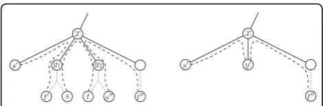
such that (without loss of generality) s∈V(Ty1)and t∈V(Ty2). Let v[s,t]denote the vertex ofGc correspond-ing to [s,t]. First, note that by the assumption that Rule (1) does not apply,v[s,t]has degree at least two.
More-over, by the choice ofxthere is no pair with both end-points inV(Ty1)or inV(Ty2). Thus, every pair that is in conflict with [s, t] uses either the edge {x, y1} or the
edge {x, y2}. Thus, since me ≤ 2 and degGc(v[s,t])≥2, there are exactly two pairsp’= [s’,t’], p’’ = [s’’, t’’]Î P that are in conflict with [s, t]. Assume without loss of generality that t ∈V(Ty1)and s ∈V(Ty2)(see Figure 1 for an illustration). Since Rule (2) does not apply to v[s,t], we can assume that p’and p’’ are not in conflict
x
y1 y2
s t
t s t
s
x
t y
s
with each other. Hence, Rule (3) can be applied tov[s,t].
LetGcdenote the graph that results by first making the two neighbors ofvadjacent and subsequently deletingv. It remains to show how to transform the MTO instance such that the conflict graph of the new instance is iden-tical toGc. To this end, consider the MTO instance that results by deleting the vertices in V(Ty1)∪V(Ty2), removing the pairs [s, t], [s’, t’], and [s’’, t’’] and subse-quently adding a vertexy’, makingy’adjacent tox, and adding the pairs [s’,y’] and [y’,t’’] (see Figure 1 for an illustration). Clearly, [s’, y’] and [y’,t’’] are in conflict. Moreover, since only the pairs p, p’, andp’’ have end-points inV(Ty1)∪V(Ty2), this transformation does not change the conflicts with the other pairs. Further, we have thatme≤2 in the resulting MTO instance.
Since width-two tree decompositions can be con-structed in linear time [21] and weighted VERTEX COVER can be solved in linear time on graphs with constant treewidth [15], this yields linear-time solvability for WEIGHTEDMAXIMUMTREEORIENTATIONwithme≤2.
Theorem 4. If me≤2,then WEIGHTEDMAXIMUM TREE ORIENTATIONcan be solved in linear time.
Proof. To be able to determine the path between a pair [s,t] inO(n) time, we root the tree arbitrarily and calcu-late in linear time a data structure that allows least com-mon ancestor queries in constant time [12]; the path can then be found by going upwards froms andtuntil hitting their least common ancestor, and then joining the two partial paths. We then construct the conflict graph by marking for each path the corresponding edges with the pair and the direction, and then register-ing a possible conflict for each tree edge. Since there can be only linearly many markings and conflicts, the construction takes O(n) time. A tree decomposition of width two can then be found in linear time [21], and, as mentioned above, solving weighted VERTEXCOVER on a graph with treewidth at most two takes only linear time, too [15]. □
We can further prove that for me ≥3, MTO is NP-hard even on stars, that is, on trees where all leaves are attached to the same vertex. The proof is by reduction from MAXDICUT.
Theorem 5. MAXIMUMTREEORIENTATIONon stars with me≥3 is NP-complete.
Proof. As Medvedovsky et al. [3] pointed out, the NP-hard MAXDICUT problem, defined as follows, can be reduced to MTO on stars.
MAXDICUT
Given a directed graph G = (V,A) and a nonnegative integer k, is it possible to find a subset of vertices C
⊆Vsuch that there are at least |A| -karcs (v,w)Î
AwithvÎCandw∉C?
From a MAXDICUTinstance (G= (V, A),k), one con-structs an equivalent MTO instance (T = (V’,E), P, k) by setting V’:=V∪ {r},E := {{v, r} |vÎV}, andP :=A, wherer∉Vis a new root vertex [3]. Clearly, if a
MAXDI-CUT instance has maximum degree three, then it
reduces to an MTO instance with me ≤ 3. Thus, it remains to show that MAXDICUTwith maximum degree three is NP-hard. (Unfortunately, there seems to be no apt reduction from the undirected version MAXCUT, which is NP-hard for maximum degree three [22].)
MAXDICUT can also be formulated as the problem to delete up tokarcs to obtain a graph where every vertex is only startpoint or only endpoint of arcs. We can char-acterize such graphs by a forbidden substructure con-sisting of three vertices u, v, w connected by the arcs (u, v) and (v,w) (the arcs (u, w) and (w,u) may or may not be present). Thus, if we ignore graphs with multiple arcs between two vertices, we have three forbidden induced subgraphs on three vertices. In this way, MAX-DICUTis similar to the TRANSITIVITY DELETION problem [23], which given a directed graph, asks for up to karc deletions to make it transitive, that is, to fulfill for allu, v, w ÎV that (u, v) Î A ∧ (v, w) Î A ⇒ (u, w) Î A. Transitive graphs are characterized by two of the three forbidden subgraphs for MAXDICUT; the subgraph with {(u, v), (v,w), (u,w)}⊆Ais not forbidden. However, if we examine the directed graphs that are produced in the reduction from 3-SAT that proves NP-hardness of TRANSITIVITYDELETION[23, Sect. 3.1], we notice that this substructure does not occur, and cannot be created by arc deletions. Thus, solving TRANSITIVITY DELETION and MAXDICUTon these directed graphs is equivalent. Since the constructed instances also have degree at most three, we obtain the NP-hardness of MAXDICUT with maximum degree three. It is easy to see that MTO is contained in NP, so we obtain the claimed theorem. □
requires an arbitrary parameter choice not documented by Medvedovsky et al. [3].)
The resulting tree is, as already observed by Medve-dovsky et al. [3], very star-like: there is one vertex of degree 1,151 and 1,048 degree-one vertices attached to it. The remaining 229 vertices have degree 1 to 4. All paths connecting cause-effect pairs pass through the central vertex.
We first note that this MTO instance is actually fairly easy to solve exactly. The Integer Linear Program (ILP) by Medvedovsky et al. [3, Sect. 3.1] and VERTEXCOVER on the conflict graph solved by either an ILP or a simple branching strategy with data reduction all solve the instance in less than a second. More precisely, the run-ning times are 0.09 s, 0.02 s, and 0.13 s, respectively, on a 2.67 GHz Intel Xeon W3520 machine, using GLPK 4.44 for the ILPs, and with the branching strategy implemented in Objective Caml. The branching strategy finds a vertex vof maximum degree and branches into the two cases of takingvinto the vertex cover or taking all neighbors of vinto the vertex cover. Before each branch, degree-1 vertices are eliminated by taking their neighbor into the vertex cover. The search in the second branch is cut short when the accumulated vertex cover is larger than that of the first branch.
Note that all three algorithms do not require the para-meter k(number of unsatisfied pairs) as input, but will determine the minimumksuch that there is a solution.
The reason that these strategies work so well is prob-ably due to the low value of the parameter k: only 77 cause-effect pairs cannot be satisfied. This limits the size of the branch-and-bound tree that underlies all three methods.
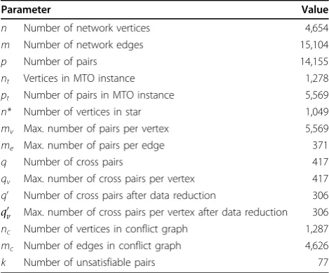
In Table 1, we examine several other parameters. Since there are stillpt= 5,569 pairs left after contracting all cycles in the network, using this parameter for a fixed-parameter algorithm seems infeasible. Unfortu-nately, since all paths run through a single vertex, the parametermvis not any more useful. Only about 5% of the pairs are cross pairs after the data reduction, soqis already a more promising parameter. However, with a value ofq = 417, this parameter seems not very helpful. Even if we eliminate pairs that do not conflict with any other pairs, leaving onlync= 1,287 pairs, we still find at least 306 cross pairs (parameter q’). Again, because all paths run through a single vertex, considering cross pairs per vertex does not help here. In summary, for this particular instance the number of unsatisfiable pairs kis clearly the most useful parameter.
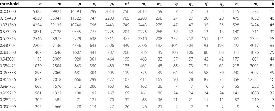
To examine the effect of the sparseness of the input instance on the various parameters, we investigated another yeast protein interaction network assembled by Nir Yosef from various sources (see references in [25]). In this network, each edge is annotated with a probability of
interaction. Thus, by thresholding, we can obtain graphs of different sparseness. The results are shown in Table 2.
We see that, here, the parameter k is not always a clear winner. When the network becomes sparser, the components that will be shrunk to a single vertex by the cycle contraction will be smaller, leaving fewer pairs with both endpoints on the same tree vertex, and thereby increasing the number of potential conflicts. Only for very high thresholds, the parameter becomes small again, since then the original instance is already much smaller. Still, all instances can be solved in less than one second by the three algorithms mentioned above, which exploit low values ofk.
We also see that for denser graphs, the parameter values based on the number of cross pairs are quite low, e.g.qv = 3 for the whole graph. Thus, it seems likely that these instances can be quickly solved by the algo-rithm from Theorem 3, running inO(2qv·n2·q
v)time.
One possible explanation for the low value for these parameters is that the networks exhibit a linear struc-ture. For example, if each protein can be assigned a dis-tance to the nucleus, and interactions mostly transport information to or from the nucleus, then we would expect to have only few cross pairs.
The parameter mv could be expected to be not too high in biological networks, since otherwise this would make the network less robust, since elimination of one vertex would disrupt too many paths. However, one ver-tex in the tree under consideration can actually corre-spond to a very large component in the original graph, which weakens this effect. Therefore, this parameter is more useful in sparser graphs, where not too many graph vertices are joined into a tree vertex. However, for the given instances, it seems small enough to be Table 1 Network parameters
Parameter Value
n Number of network vertices 4,654 m Number of network edges 15,104
p Number of pairs 14,155
nt Vertices in MTO instance 1,278 pt Number of pairs in MTO instance 5,569 n* Number of vertices in star 1,049 mv Max. number of pairs per vertex 5,569 me Max. number of pairs per edge 371
q Number of cross pairs 417
qv Max. number of cross pairs per vertex 417 q’ Number of cross pairs after data reduction 306
qv Max. number of cross pairs per vertex after data reduction 306 nc Number of vertices in conflict graph 1,287 mc Number of edges in conflict graph 4,626 k Number of unsatisfiable pairs 77
exploited only for fairly small instances, where other parameters would give good results, too.
The parameter mecould similarly be expected to be low in sparse networks; however, the NP-hardness result already for me≥ 3 (Theorem 5) makes practical use of this parameter unlikely.
Conclusions
We started a parameterized complexity analysis of (WEIGHTED) MAXIMUM TREE ORIENTATION, obtaining a more fine-grained view on the computational complex-ity of this NP-hard problem. In this line, there are still several challenges for future investigations. For instance, it is open whether MTO is fixed-parameter tractable with respect to the parameter “number of satisfied pairs” (n - k). Further, in the spirit of “ dis-tance-from-triviality parameterization” [19,20] it would be interesting to study the parameterized complexity of MTO with respect to the parameter“number of all possible pairs minus the number of input pairs"–recall that for parameter value zero MTO is polynomial-time solvable [11]. MTO restricted to stars is still NP-hard, but then at least one quarter of all input pairs can always be satisfied [3]. Hence, it would be interesting to study above guarantee parameterization [15,20] with respect to the number of satisfied pairs. MTO can be translated into a vertex covering problem (see Proposi-tion 1) on a graph class that is K4-free–this motivates
to study whether vertex covering on this graph class can be done faster than on general graphs. Clearly, MTO brings along numerous further parameters and parameter combinations which can make a more com-prehensive multivariate complexity analysis [20] very
attractive. Often, it is desirable to not only list a single solution, but to enumerate all optimal solutions. Our dynamic-programming-based algorithms seem suitable for this. Following Gamzu et al. [8] and extending the studies for MTO as pursued here to the more general case of mixed graphs with partially already oriented edges is of high interest. First steps in this direction have very recently been undertaken by Silverbush et al. [9] and Elberfeld et al. [26]. Finally, it seems promising to examine the parameters based on cross pairs in other networks such as communication networks, and to try to exploit these parameters for other hard net-work problems.
Acknowledgements
A preliminary version of this work appeared in the proceedings of the 1st International ICST Conference on Theory and Practice of Algorithms in (Computer) Systems (TAPAS‘11), volume 6595 in Lecture Notes in Computer Science, pages 104-115, Springer 2011.
JU and partly FH were supported by the Deutsche Forschungsgemeinschaft (DFG), research project PABI (NI 369/7).
Major parts of the work were done while BD and DK were with the Universität Tübingen, FH was with the Humboldt-Universität zu Berlin, and RN and JU were with the Friedrich-Schiller-Universität Jena. We are grateful to two anonymous referees whose insightful remarks helped to improve the presentation of our work.
Author details
1Fakultät für Mathematik und Wirtschaftswissenschaften, Universität Ulm, Ulm, Germany.2Institut für Softwaretechnik und Theoretische Informatik, TU Berlin, Berlin, Germany.3Institut für Theoretische Informatik, Universität Ulm, Ulm, Germany.
Authors’contributions
All authors contributed more or less equally, RN initiating the study of MTO under the viewpoint of multivariate complexity analysis and JU coming up with the major algorithmic ideas which have been worked out in more detail by DK. All authors read and approved the final manuscript. Table 2 Thresholded network parameters
threshold n m p nt pt n* mv me q qv q’ qv nc mc k
0.000000 5385 39921 14393 799 2014 750 2014 59 7 7 3 3 115 292 17 0.154420 4530 35041 11522 747 2203 705 2203 298 27 27 20 20 475 1632 40 0.371369 4254 32135 10740 796 2443 749 2443 275 47 47 35 35 528 2424 46 0.573290 3871 27128 9445 777 2225 704 2225 268 32 32 13 13 140 311 32 0.573313 2546 8977 5279 638 2311 477 2310 208 252 252 151 151 561 2394 68 0.830093 2206 7136 4346 643 2206 449 2206 192 304 304 193 193 727 4017 83 0.886308 1407 3646 1607 441 787 260 785 45 106 106 88 88 311 1876 75
0.943001 1135 3069 920 361 464 195 463 32 57 57 42 42 179 801 44
0.954421 1039 2504 843 350 489 175 461 45 85 73 71 61 215 3001 81
0.957338 895 2060 681 304 405 119 375 39 64 54 58 50 240 3092 89
0.965986 874 2018 666 299 477 103 411 165 90 78 85 75 358 12284 110
0.984753 668 1676 312 206 163 95 162 20 7 7 6 6 55 222 15
0.989212 581 1322 188 192 167 69 161 86 24 24 24 24 141 1088 32
0.989233 307 681 71 121 70 32 66 36 21 21 11 11 52 219 7
0.990409 294 666 28 114 27 26 26 21 2 2 2 2 9 8 2
Competing interests
The authors declare that they have no competing interests.
Received: 22 March 2011 Accepted: 25 August 2011 Published: 25 August 2011
References
1. Werther M, Seitz H, Eds: InProtein-protein interaction. Volume 110.Advances in Biochemical Engineering/Biotechnology. Springer; 2008.
2. Yeang CH, Ideker T, Jaakkola T:Physical network models.Journal of Computational Biology2004,11(2-3):243-262.
3. Medvedovsky A, Bafna V, Zwick U,et al:An algorithm for orienting graphs based on cause-effect pairs and its applications to orienting protein networks.InProc 8th WABI. Volume 5251.LNBI, Springer; 2008:222-232. 4. Karzanov AV:Èkonomnyj algoritm nahoždeniâ bikomponent grafa [in
Russian: An efficient algorithm for finding the bicomponents of a graph].Trudy tret’ej zimnejškoly po matematičeskomû programmirovaniu i smežnym voprosam [Proceedings of the 3rd Winter School on Mathematical Programming and Related Problems]Moscow Engineering and Construction Institute (MISI); 1970, 343-347.
5. Tarjan RE:Depth-first search and linear graph algorithms.SIAM Journal on Computing1972,1(2):146-160.
6. Alm E, Arkin AP:Biological networks.Current Opinion in Structural Biology 2003,13(2):193-202.
7. Sharan R, Ideker T:Modeling cellular machinery through biological network comparison.Nature Biotechnology2006,24:427-433.
8. Gamzu I, Segev D, Sharan R:Improved orientations of physical networks. InProc 10th WABI. Volume 6293.LNBI, Springer; 2010:215-225.
9. Silverbush D, Elberfeld M, Sharan R:Optimally orienting physical networks. InProc 15th RECOMB. Volume 6577.LNBI, Springer; 2011:424-436.
10. Gitter A, Klein-Seetharaman J, Gupta A,et al:Discovering pathways by orienting edges in protein interaction networks.Nucleic Acids Research 2011,39(4):e22.
11. Hakimi SL, Schmeichel EF, Young NE:Orienting graphs to optimize reachability.Information Processing Letters1997,63(5):229-235.
12. Harel D, Tarjan RE:Fast algorithms for finding nearest common ancestors. SIAM Journal on Computing1984,13(2):338-355.
13. Downey RG, Fellows MR:Parameterized ComplexitySpringer; 1999. 14. Flum J, Grohe M:Parameterized Complexity TheorySpringer; 2006. 15. Niedermeier R:Invitation to Fixed-Parameter Algorithms.No. 31 in Oxford
Lecture Series in Mathematics and Its Applications, Oxford University Press; 2006.
16. Niedermeier R, Rossmanith P:On efficient fixed-parameter algorithms for weighted vertex cover.Journal of Algorithms2003,47(2):63-77. 17. Song Y, Liu C, Huang X,et al:Efficient parameterized algorithms for
biopolymer structure–sequence alignment.IEEE/ACM Trans Comput Biology Bioinform2006,3(4):423-432.
18. Bodlaender HL:A partial k-arboretum of graphs with bounded treewidth. Theoretical Computer Science1998,209(1-2):1-45.
19. Guo J, Hüffner F, Niedermeier R:A structural view on parameterizing problems: distance from triviality.InProc 1st IWPEC. Volume 3162.LNCS, Springer; 2004:162-173.
20. Niedermeier R:Reflections on multivariate algorithmics and problem parameterization.InProc 27th STACS. Volume 5.Leibniz International Proceedings in Informatics, Schloss Dagstuhl - Leibniz-Zentrum für Informatik; 2010:17-32.
21. Arnborg S, Proskurowski A:Characterization and recognition of partial 3-trees.SIAM Journal on Algebraic and Discrete Methods1986,7(2):305-314. 22. Yannakakis M:Edge-deletion problems.SIAM Journal on Computing1981,
10(2):297-309.
23. Weller M, Komusiewicz C, Niedermeier R,et al:On making directed graphs transitive.Journal of Computer and System Sciences2011.
24. Salwinski L, Miller CS, Smith AJ,et al:The database of interacting proteins: 2004 update.Nucleic Acids Research2004, ,32 Database:D449-D451. 25. Bruckner S, Hüffner F, Karp RM,et al:Topology-free querying of protein
interaction networks.Journal of Computational Biology2010,17(3):237-252. 26. Elberfeld M, Segev D, Davidson CR,et al:Approximation algorithms for
orienting mixed graphs.InProc 22nd CPM. Volume 6661.LNCS, Springer; 2011:416-428.
doi:10.1186/1748-7188-6-21
Cite this article as:Dornet al.:Exploiting bounded signal flow for graph orientation based on cause–effect pairs.Algorithms for Molecular Biology
20116:21.
Submit your next manuscript to BioMed Central and take full advantage of:
• Convenient online submission
• Thorough peer review
• No space constraints or color figure charges
• Immediate publication on acceptance
• Inclusion in PubMed, CAS, Scopus and Google Scholar
• Research which is freely available for redistribution