Segmentor3IsBack: an R package for the fast and exact segmentation of Seq-data

S O F T W A R E A R T I C L E

Open Access

Segmentor3IsBack: an R package for the fast

and exact segmentation of Seq-data

Alice Cleynen

, Michel Koskas

, Emilie Lebarbier

, Guillem Rigaill

and Stéphane Robin

Abstract

Background: Change point problems arise in many genomic analyses such as the detection of copy number variations or the detection of transcribed regions. The expanding Next Generation Sequencing technologies now allow to locate change points at the nucleotide resolution.

Results: Because of its complexity which is almost linear in the sequence length when the maximal number of segments is constant, and as its performance had been acknowledged for microarrays, we propose to use the Pruned Dynamic Programming algorithm for Seq-experiment outputs. This requires the adaptation of the algorithm to the negative binomial distribution with which we model the data. We show that if the dispersion in the signal is known, the PDP algorithm can be used, and we provide an estimator for this dispersion. We describe a compression framework which reduces the time complexity without modifying the accuracy of the segmentation. We propose to estimate the number of segments via a penalized likelihood criterion. We illustrate the performance of the proposed methodology on RNA-Seq data.

Conclusions: We illustrate the results of our approach on a real dataset and show its good performance. Our algorithm is available as anRpackage on the CRAN repository.

Keywords: Segmentation algorithm, Exact algorithm, Fast algorithm, RNA-Seq data, Genome annotation, Count data, Data compression

Background

Change-point detection methods have long been used in the analysis of genetic data as an efficient tool in the study of DNA sequences for various purposes. For instance, seg-mentation methods have been developed for categorical variables with the aim of identifying patterns for gene predictions [1,2], while SNPs have been detected using sequence segmentation [3]. In the last two decades, with the large spread of micro-arrays, change-point methods have been widely used for the analysis of DNA copy num-ber variations and the identification of amplification or deletion of genomic regions in pathologies such as cancer [4-8].

The recent development of Next-Generation Sequenc-ing technologies gives rise to new applications along with new difficulties: (a) the increased size of profiles (up to 108

*Correspondence: [email protected]

1AgroParisTech, UMR 518, 16 rue Claude Bernard, 75231 Paris Cedex 05, France 2INRA, UMR 518, 16 rue Claude Bernard, 75231 Paris Cedex 05, France Full list of author information is available at the end of the article

data-points when micro-array signals were closer to 105), and (b) the discrete nature of the output (number of reads starting at each position of the genome). Yet applying seg-mentation methods to DNA-Seq data with their greater resolution should lead to the analysis of copy-number variation with a much improved precision compared to CGH arrays. Moreover, in the case of poly-(A) RNA-Seq data on lower organisms, since coding regions of the genome are well separated from non-coding regions with lower activity, segmentation methods should allow the identification of transcribed genes as well as address the issue of new transcript discovery. Our objective is there-fore to develop a segmentation method to tackle both (a) and (b) with some specific requirements: the amount of reads falling within a segment should be represen-tative of the biological information associated (relative copy-number of the region, relative level of expression of the gene), and comparison to neighboring regions should be sufficient to label the segment (for instance normal or deleted region of the chromosome in DNA-Seq data, exon or non-transcribed region in RNA-Seq), therefore

no comparison profile should be needed. This also sup-presses the need for normalization, and consequently we wish to analyze the raw count-profile.

Up to now, most methods addressing the analysis of these datasets require some normalization process to allow the use of algorithms which rely on Gaussian-distributed data or which were previously developed for micro-arrays [9-12]. Indeed, methods adapted to count datasets are not numerous and are highly focused on the Poisson distribution. Alteration of genomic sequences can be detected based on the comparison of Poisson processes associated with the read counts of a case and a control sample [13], but this cannot be applied to the detection of transcribed regions in a single condition.

Still, a likelihood ratio statistic was proposed for the localization of a shift in the intensity of a Poisson process [14], and a test statistic was proposed for the existence of a change-point in the Poisson autoregression of order 1 [15]. These last two methods do not require a comparison profile but they only allow for the detection of a single change-point and have too high a time-complexity to be applied to RNA-Seq profiles. Binary Segmentation, a fast heuristic [6], and Pruned Exact Linear Time (PELT) [16], an exact algorithm for optimal segmentation with respect to the likelihood, are both implemented for the Poisson distribution in the changepoint package. Even though both are extremely fast, do not require a comparison pro-file, and analyze count-data, the Poisson distribution is not adapted to our kind of datasets.

A recent study [17] has compared 13 segmentation methods for the analysis of chromosomal copy number profiles and has shown the excellent performance of the Pruned Dynamic Programming (PDP) algorithm [18] pro-posed in its initial implementation for the analysis of Gaussian data in the Rpackage cghseg. We propose to use this algorithm, which we have implemented for the Poisson and negative binomial distributions.

In the next section we recall the general segmentation framework and the definition and requirements of the PDP algorithm. Our contributions are given in the third section where we define the negative binomial model and show that it satisfies the PDP algorithm requirements. We also provide a theoretical result for the possibility to compress the data, and finally we give a model selection criterion with theoretical guarantees, which makes the whole approach complete. We conclude with a simulation study, which illustrates the performance of the proposed method.

Segmentation model and algorithm General segmentation model

The general segmentation problem consists in partition-ing a signal ofndata-points{yt}t∈[[1,n]]into a given number K of pieces or segments. The model can be written as

follows: the observed data{yt}t=1,...,nare supposed to be a realization of an independent random process Y = {Yt}t=1,...,n. This process is drawn from a probability dis-tributionGwhich depends on a set of parameters among which one parameterθ is assumed to be affected byK−1 abrupt changes, called change-points, such that

Yt∼G(θr,φ) if t ∈ r and r∈m

wheremis a partition of [[ 1,n]] into segmentsr,θrstands for the parameter of segment r and φ is constant. The objective is to estimate the change-points or the posi-tions of the segments and the parametersθrboth resulting from the segmentation. More precisely, we define Mk,t the set of all possible partitions ink > 0 regions of the sequence up to point t. We recall that the number of possible partitions is

card(Mk,t)=

t−1 k−1

.

We aim at choosing the partition in MK,n of minimal loss γ, where the loss is usually taken as the nega-tive log-likelihood of the model. We define the point-additive loss of a segment with given parameter θ as c(r,θ)=_i∈rγ (yi,θ), therefore its optimal cost isc(r)= minθ{c(r,θ)}. This allows us to define the cost of a seg-mentationmas_r∈mc(r)and our goal is to recover the optimal segmentation MK,n and its cost CK,n which are particular cases of the generic optimal segmentation of the signal up to pointtinksegments and its cost, defined as:

Mk,t = arg min{m∈Mk,t}

r∈m c(r)

and Ck,t = min{m∈Mk,t}

r∈m c(r)

.

Quick overview of the PDP algorithm

Like the original DP algorithm, the pruned DP algorithm is an iterative algorithm based on the minimization of a cost functionCk,twhich is traditionally decomposed as:

Ck,t= min

{k−1<τ<t}

Ck−1,τ+min

θ [c([τ+1,t],θ)] (1)

whereθ is the parameter of the cost of the last segment, constraints on its possible values being directly related to the support of the loss functionγ (for instanceθtakes its value in Rin the case of the Gaussian loss, but in [0, 1] in the case of the binomial loss). In what follows we will denote byIsthe set of possible values for parameterθ.

The specificity of the PDP algorithm is that it relies on the comparison of candidates for the last change-point positionτ through the permutation of the minimizations in (1) and the introduction of the functions:

Hk,t(θ)= min

k−1<τ≤t

which are the cost of the best partition inkregions up to t, the parameter of the last segment beingθ.Ck,t is then obtained as minθ{Hk,t(θ)}.

Then at each iterationk, the PDP algorithm works on a list of last change-point candidates: ListCandidatek. For each of theseτs and for each value oft, it updates the set ofθs, denotedSτ_k,t for which this candidate is optimal. If this set is empty, the candidate is discarded, resulting in the pruning and lower complexity of the algorithm.

The foundations of the algorithm can be written as follows.

• DefiningH_kτ_,t(θ)=Ck−1,τ +tj=τ+1γ (yj,θ)the optimal cost if the last change isτ and last parameter isθ, then

(i ) H_kτ_,t+1(θ)is obtained fromH_kτ_,t(θ)using:

H_kτ_,t+1(θ)=H_kτ_,t(θ)+γ (yt+1,θ);

• DefiningI_kτ_,t=θ |H_kτ_,t(θ) ≤ H_kt_,t(θ)=

θ |H_kτ_,t(θ) ≤ Ck−1,t

the set ofθsuch thatτ is better thant in terms of cost, withτ <t, then

(ii ) if allt_j=τ+1γ (yj,θ)are unimodal inθ thenI_kτ_,t are intervals. Indeed, since by definition H_kt_,t(θ)=Ck−1,tand the cost function does not depend onθ,I_kτ_,tis the set of values for which a unimodal function is smaller than a constant.

• Finally, we introduceSτ_k,t=

θ|H_kτ_,t(θ) ≤ Hk,t(θ)

the set ofθsuch thatτ is optimal. Then since Hk,t(θ)=minτ≤t

H_kτ_,t(θ)

,Sτ_k,tcan be written as

θ |H_kτ_,t(θ) = Hk,t(θ)

and we obtain that

(iii ) Sτ_k,t+1can be updated using:

Sτ_k,t+1=S_kτ_,t ∩I_kτ_,t+1

St_k,t=Is\(∪τ∈ListCandidatekI τ k,t)

The first assertion follows from the fact that Sτ_k,t+1=

θ|H_kτ_,t+1≤mink≤τ≤t+1H_kτ_,t+1

=

θ|H_kτ_,t+1≤min

H_kt+1_,t+1, mink≤τ≤tH_kτ_,t+1

, the first term in the minimum givingI_kτ_,t+1and the second one givingSτ_k,t. The second assertion trivially follows from the fact that candidatet is optimal on the set of values where no other candidate was optimal.

(iv) once it has been determined thatSτ_k,tis empty, it easily follows from the update equation(iii)that the region-borderτ can be discarded from the list of candidatesListCandidatek:

Sτ_k,t= ∅ ⇒ ∀t≥t Sτ_k,t = ∅.

Requirements of the pruned dynamic programming algorithm.

Proposition 0.1. Properties (i) to (iv) are satisfied as soon as the following conditions on the loss c(r,θ)are met:

(a) It is point additive,

(b) It is convex with respect to its parameterθ, (c) It can be stored and updated efficiently.

The proof of those claims can be found in [18]. A pseudo-code of the PDP algorithm is given in the appendix.

It is possible to include an additional penalty term, denotedgas in the pseudo-code, in the loss function. To preserve the point-additivity requirement of the loss, this penalty can only depend on the value of the segment-parameter θ and not on any other characteristics, such as segment length. This is then equivalent to minimizing

Ck,t = min{k−1<τ<t}

Ck−1,τ+minθc([τ+1,t] ,θ)+g(θ)

and can be achieved by adding the penalty valueg(θ)in the initialization of H_kτ_,t(θ). For example, in the case of RNA-seq data one could add a lasso (λ|θ|) or ridge penalty (λθ2) to encode thata priorithe coverage in most regions should be close to 0. Our C++ implementation of the PDP algorithm includes the possibility of adding such a penalty term; however we do not provide anR interface to this functionality in ourRpackage. One of the reasons for this choice is that choosing an appropriate value forλis not a simple problem.

Contribution

Pruned dynamic programming algorithm for count data We now show that the PDP algorithm can be applied to the segmentation of RNA-Seq data using a negative bino-mial model and we propose a criterion for the choice ofK. Though not discussed here, our results also hold for the Poisson segmentation model.

Negative binomial model. We consider that in each seg-mentr all yt are the realization of random variablesYt which are independent and follow the same negative bino-mial distribution. Assuming the dispersion parameter φ to be known, we will use the natural parametrization from the exponential family (also classically used in R) so that parameterθrwill be the probability of success. In this framework,θr is specific to segment rwhereasφ is common to all segments.

Validity of the pruned dynamic programming algo-rithm for the negative binomial model

Proposition 0.2. Assuming parameterφto be known, the negative binomial model satisfies (a), (b) and (c):

(a) As we assume thatYtare independent, we indeed have that the loss is point additive:c(r,θ)=

t∈rγ (yt,θ).

(b) Asγ (yt,θ)= −φlog(θ)−ytlog(1−θ)is convex with respect toθ,c(r,θ)is also convex as the sum of convex functions.

(c) Finally, we have c(r,θ)= −nrφlog(θ)+ t∈rytlog(1−θ)(wherenris the length of segmentr). This function can be stored and updated using only two doubles: one for−nrφ, sayd1, and the

other for_t∈ryt, sayd2. Then at stept+1as the

new datapointyt+1is considered, these doubles are simply updated asd1←d1+φandd2←d2+yt+1.

Estimation of the overdispersion parameter. We pro-pose to estimateφ using a modified version of Johnson et. al’s estimator [19]: compute the moment estimator of

φ on each sliding window of size h using the formula

φ=E(Y)2_{/(Var(Y)−E(Y))and keep the medianφ.}

Taking into account a positional bias. It is possible that the assumption that the counts share the same distribu-tion in a segment might not be verified. For instance in the case of RNA-Seq data the number of reads can be affected by the location in the transcribed region or by the GC-content of the fragment. The pruned dynamic pro-gramming algorithm only requires a vector of integers as input, it is therefore possible to apply any kind of normal-ization process that preserves the count-specificity of the data prior to segmentation. For instance, a method such as that which has resulted in the publication of the data used in the illustration [20] can be applied. A comparison of the main normalization methods can for example be found in Bullardet. al.’s paper [21].

C++ implementation of the PDP algorithm

We implemented the PDP algorithm in C++ having in mind the possibility of adding new loss functions in poten-tial future applications. The difficulties we had to face were the versatility of the program to be designed and the design of the objects it could work on. Indeed, the use of full templates implied that we used stable sets of objects for the operations that were to be performed.

Namely:

• The sets were to be chosen in atribe. This means that they all belong to a setSof sets such that any set s∈Scan be conveniently handled and stored in the

computer. A set of setsSis said to beacceptable if it satisfies the following:

1. Ifs belongs toS,R\s∈S 2. Ifs1,s2∈S, s1∩s2∈S

3. Ifs1,s2∈S, s1∪s2∈S

For instance, the setSof intervals is a tribe since the complementary, the union and the intersection of intervals form a union of intervals. This property ensures that the setsI_kτ_,tandS_kτ_,tcan be updated and stored efficiently (only two doubles are required to store an interval) to take full advantage of the pruning process.

• The cost functions were chosen in a setFsuch that

1. Each function may be conveniently handled and stored by the software.

For instance, for the Gaussian loss it suffices to store the three coefficients of a second order polynomial.

2. For anyf ∈Fand any constantc,f(x)≤ccan be easily solved and the set of solutions belongs to an acceptable set of sets

3. For anyf,g∈F,f +g∈F.

These two points ensure that the cost (and penalty) functions can be easily updated and compared so that the setsIτ_k,tof each candidateτ can be updated and candidates eventually discarded.

Thus we defined two collections for the sets of setsS, intervals and parallelepipeds, and implemented the loss functions corresponding to negative binomial, Poisson or normal distributions. The program is thus designed in a way that any user can add his own cost function or acceptable set of probability function and use it without rewriting a line in the code.

Compression of the signal

In the case of count data, and in particular in the analysis of RNA-Seq data, it is very likely that we observe plateaux, that is regions between two arbitrary positionst1andt2 (>t1) where the signal is constant:

∀t, t1≤t≤t2, yt=yt1=yt2.

Then we have the following proposition, the proof of which is given in the appendix.

Proposition 0.3. There exists a segmentation m in K or fewer segments without any change-point in the plateaux such that the optimal cost of m is equal to CK,n.

look for change-points in plateaux. In other words a plateau starting at positiont1and ending at positiont2can be considered as a unique data point with valueyt1 and weightt2−t1+1. At worst the size of the compressed sig-nal is equal to the minimum between two times the num-ber of reads and the length of the chromosome arm. Thus, if the number of reads is very large, the two-step algorithm (compression and pruned dynamic programming) does not change the worst case complexity. However, in most cases the number of reads is much smaller than the size of the considered chromosome. Thus compression is effi-cient and allows for a significant reduction in the overall run-time. Furthermore, in the case of RNA-Seq data we do not expect reads to be evenly scattered. On the contrary they are concentrated in transcribed regions and between those regions we expect large plateaux of 0 allowing for an efficient compression (for instance only 2% of the human chromosome contains coding regions).

Model selection

The last issue concerns the estimate of the number of seg-mentsK. This model selection issue can be solved using a penalized log-likelihood criterion for which the choice of a good penalty function is crucial. This kind of procedure typically requires computation of the optimal segmen-tations in all k = 1,. . .,Kmax segments where Kmax is generally chosen smaller thann. The most popular cri-teria (AIC [22] and BIC [23]) failed in the segmentation context due to the discrete nature of the change-points. Indeed, additionally to being an asymptotic criterion in a framework where the collection of possible models grows polynomially with n, the BIC criterion uses a Laplace approximation requiring differentiability conditions of the likelihood function which are not satisfied by the seg-mentation model [24]. From a non-asymptotic point of view and for the negative binomial model, the follow-ing criterion was proposed [25]: denotfollow-ingmˆKthe optimal segmentation of the data inKsegments,

ˆ

K= arg min K∈1:Kmax

⎧ ⎨ ⎩

r∈ ˆmK

t∈r

−φlog φ φ+ ¯yr −

ytlog

1− φ

φ+¯yr

+βK

1+4

1.1+logn

K

2⎫⎬ ⎭,

(2)

wherey¯r =

t∈ryt

ˆ nr

andnˆr is the size of segmentr. The first term corresponds to the cost of the optimal segmen-tation while the second is a penalty term which depends on the dimensionK and on a constantβ that has to be tuned according to the data (see the next section). With this choice of penalty, a so-called oracle penalty, the result-ing estimator satisfies an oracle-type inequality. A more complete performance study is done in [25] and showed that the proposed criterion outperforms the existing ones.

Implementation

The Pruned Dynamic Programming algorithm is available in the functionSegmentor of theRpackage Segmen-tor3IsBack. Version 1.7 of this package contains the com-pression process which is performed by default in the case of count data. The user can choose the distribution with the slotmodel(1 for Poisson, 2 for Gaussian homoscedas-tic, 3 for negative binomial and 4 for segmentation of the variance). It returns an S4 object of class Segmen-tor which can later be processed for other purposes. The functionSelectModelprovides four criteria for choos-ing the optimal number of segments: AIC [22], BIC [23], the modified BIC [24] (available for Gaussian and Poisson distribution) and oracle penalties (available for the Gaus-sian distribution [26] and for the Poisson and negative binomial [25] as described previously). This latter kind of penalty requires tuning a constant according to the data, which is done using the slope heuristic [27].

Figure 1 (which is detailed in the Results and discussion Section) was obtained with the following 4 lines of code (assuming the data was contained in vectorx):

Seg<-Segmentor(x,model=3,Kmax=200)

Kchoose<-SelectModel(Seg, penalty= "oracle")

plot(sqrt(x),col=’dark red’)

abline(v=getBreaks(Seg)[Kchoose, 1:Kchoose],col=’blue’)

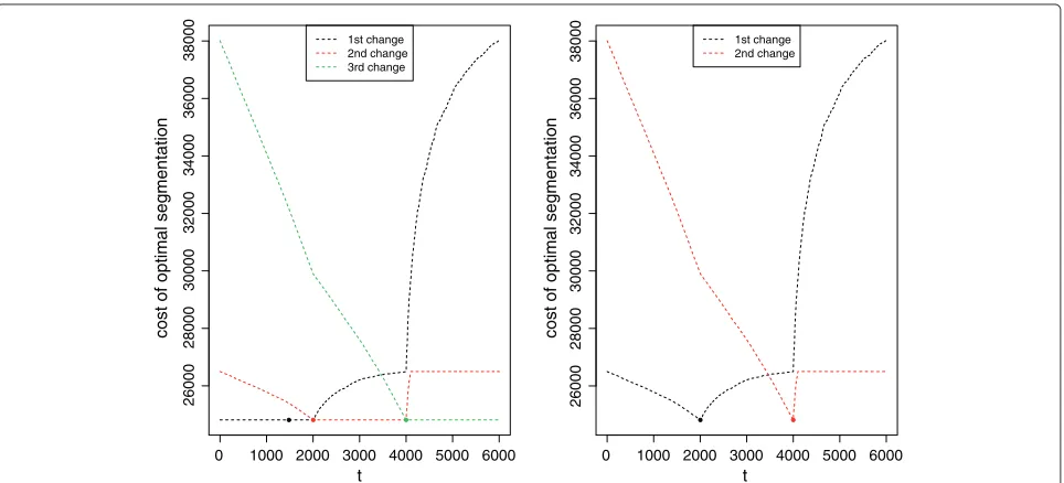
The function BestSegmentation allows us, for a

givenK, to find the optimal segmentation with a change-point at location t (slot $bestSeg). It also provides, through the slot $bestCost, the cost of the optimal segmentation witht forjth change-point. Figure 2(Left) illustrates this result for the optimal segmentations in 4 segments of a signal simulated with only 3 segments. We can see for instance that any choice of first change-point location between 1 and 2000 yields almost the same cost (the minimum is obtained fort = 1481), and thus the optimal segmentation is not clearly better than the next best segmentations. On the contrary, the same function with 3 segments shows that the optimal segmentation outperforms all other segmentations in 3 segments.

Results and discussion Performance study

Figure 1Segmentation of the yeast chromosome 1 using the negative binomial loss.The model selection procedure choosesK=125 segments, most of which correspond to the official annotation, with segments corresponding to transcribed regions surrounding official genes.

of maximum, quasi-maximum likelihood and moment estimators) on several real RNA-Seq data (whole chro-mosome and genes of various sizes), we fixed φ1 = 0.3 as a typical value for highly dispersed data as observed in real RNA-Seq data and chose φ2 = 2.3 for compari-son with a reacompari-sonably dispersed dataset. For each value, we simulated datasets of sizenwith various densities of number of segments K, and only two possible values for the parameterpJ: 0.8 on even segments (corresponding to low signal) and 0.2 on odd segments for a higher signal. We hadn vary on a logarithmic scale between 103and

106andKbetween√n/6 and√n/3. For each configura-tion, we segmented the signal up to Kmax = √ntwice: once with the known value ofφ and once with our esti-matorφas described above. We started with a window widthh= 15. When the estimate was negative, we dou-bledhand repeated the experience until the median was positive.

Each configuration was simulated 100 times.

For our analysis we checked the run-time on a standard laptop, and assessed the quality of the segmentation using the Rand Index I. Specifically, let Ct be the true index

t

cost of optimal segmentation

1st change 2nd change 3rd change

0 1000 2000 3000 4000 5000 6000

38000

0 1000 2000 3000 5000 6000

38000

t

cost of optimal segmentation

1st change 2nd change

36000

34000

32000

30000

28000

26000

36000

34000

32000

30000

28000

26000

4000

Figure 2Cost of optimal segmentation in 4 and 3 segments.Cost of optimal segmentation depending on the location of thejth_change-point

of the segment to which basetbelongs and letCˆtbe the index estimated by the method, then

I=2

n

s=1

t>s

1Ct=Cs1Cˆt= ˆCs+1Ct=Cs1Cˆt= ˆCs

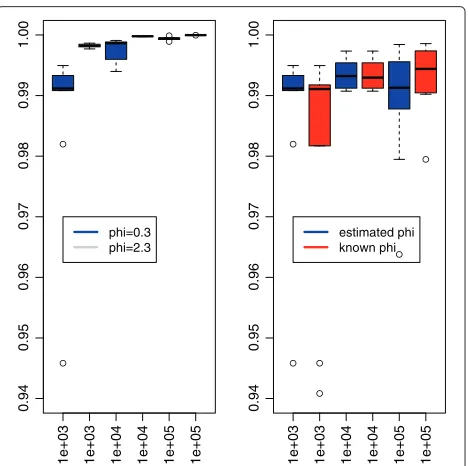
(n−1)(n−2) . Figure 3 shows, for the particular case ofK =√n/3, the almost linear complexity of the algorithm in the sizenof the signal. As the maximal number of segmentsKmax con-sidered increased withn, we normalized the run-time to allow comparison. This underlines an empirical complex-ity smaller thanO(Kmaxnlogn), and independent of the value ofφor its knowledge. Moreover, the algorithm, and therefore the pruning, is faster when the overdispersion is high, a phenomenon already encountered with theL2 loss when the distribution of errors is Cauchy. However, the knowledge of the true value ofφ does not affect the run-time of the algorithm. Figure 4 illustrates through the Rand Index the quality of the proposed segmentation for a few values ofn. Even though the indexes are slightly lower for φ1 than for φ2 (see left panel), they range between 0.94 and 1 showing a great quality in the results. More-over, the knowledge ofφdoes not increase the quality (see right panel), which validates the use of our estimator. We can therefore conclude that the run-time of our algorithm without compression is roughly 40×Kmax×n/106s.

Yeast RNAseq experiment

We applied our algorithm to the segmentation of chromo-some 1 of theS. Cerevisiae(yeast) using RNA-Seq data

0e+00 2e+05 4e+05 6e+05 8e+05 1e+06

01

0

2

0

3

0

4

0

signal size

time/Kmax (s)

phi=0.3, unknown phi=0.3, known phi=2.3, unknown phi=2.3, known

Figure 3Run-time analysis for segmentation with negative binomial distribution.This figure displays the normalized (byKmax) run-time in seconds of theSegmentor3IsBackpackage for the segmentation of signals with increasing lengthn, for two values of the dispersionφ, and with separate analyses for a known value or an estimated value. While the algorithm is faster for more over-dispersed data, the estimation of the parameter does not slow the processing.

0.94

0.95

0.96

0.97

0.98

0.99

1.00

phi=0.3 phi=2.3

1e+03 1e+03 1e+04 1e+04 1e+05 1e+05

0.94

0.95

0.96

0.97

0.98

0.99

1.00

estimated phi known phi

1e+03 1e+03 1e+04 1e+04 1e+05 1e+05

Figure 4Rand Index for the quality of the segmentation.This figure displays the boxplot of the Rand Index computed for each of the hundred simulations performed in the following situations: comparing the values withφ1andφ2when estimated (left figure), and comparing the impact of estimatingφ1(right figure). While the estimation does not decrease the quality of the segmentation, the value of the dispersion affects the recovery of the true change-points.

from the Sherlock Laboratory at Stanford University [20], publicly available from the NCBI’s Sequence Read Archive (SRA, http://www.ncbi.nlm.nih.gov/sra, accession num-ber SRA048710). We selected the numnum-ber of segments using our oracle penalty described in the previous section. An existing annotation of translated regions (i.e. exclud-ing un-translated regions (UTR)) is available on the Saccharomyces Genome Database (SGD) at http://www. yeastgenome.org, which allows us to validate our results.

With a run-time of 27 minutes without compression, and 5.4 minutes with compression (for a signal length of 230218), we selected 125 segments with the negative binomial distribution. Most of those segments (all but 3) can be related to the official annotation, however as expected segments corresponding to transcribed regions (as opposed to intergenic regions) were found to surround known genes from the SGD due to the difference between transcribed and translated regions. Figure 1 illustrates the result.

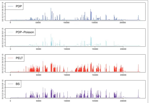
fair comparison, we also used the PDP algorithm for the Poisson loss. Figure 5, together with Table 1 which gives the estimated number of segments, the overall Hellinger score_tHt/n

and the number of change-points falling within annotated translated regions, illustrates the result and shows that we outperform the other approaches. Moreover, most of the Hellinger peaks observed can be explained by the fact that we are comparing the annotation of transcribed regions with that of translated regions.

Analysis of complex organisms

The issues raised in the analysis of RNA-Seq and DNA-Seq data differ. In the first case, the number of seg-ments that we hope to select is roughly twice the number of expressed exons, therefore the order of Kmax varies from 102(small chromosomes from lower organisms, e.g. yeast) to 104 (large chromosomes from higher organ-isms, e.g. human). However, when aligned to a refer-ence genome, RNA-Seq data is expected to present large plateaux of zeros at non-coding regions (for instance, 98%

Table 1 Comparison of algorithm performance on real data

Algorithm Number of Hellinger False

segments score positives

PDPA- negative binomial 125 0.0120 39

PDPA- Poisson 106 0.0187 77

PELT 3416 0.0188 3003

Binary Segmentation 2408 0.0151 2072

Overall Hellinger score of each of the segmentation algorithms, and number of estimated change-points falling within regions annotated as translated (thus considered as false positives).

of the human genome) and at non expressed regions. The compression option of our algorithm then allows us to reduce the size of the profile by a factor of 10 to 103. Moreover, it is well-known that centromere regions are large non-coding regions where no change-point is expected, and we therefore propose to divide the profile into two parts at such regions. As a proof of concept we ran our algorithm with compression on an RNA-seq pro-file of the small arm of the 4th chromosome ofArabidopsis

0 50000 100000 150000 200000

PDP

0 200000

PDP−Poisson

0 150000 200000

PELT

0 50000 105000 200000

1.0

1.0

1.0

1.0

BS

100000 100000 50000

150000 100000

0.8

0.6

0.4

0.2

0.0

0.8

0.6

0.4

0.2

0.8

0.6

0.4

0.2

0.0

0.8

0.6

0.4

0.2

0.0

0.0

50000

Thaliana n=4.106, Kmax=6.103

and selected 4289 segments after a compression factor of 10 and a run-time of 19 hours on a 2.4Ghz computer. The data was kindly provided by some of our collaborators.

DNA-Seq data on the other hand will present much smaller plateaux. While this implies that the compression will be less efficient, the profile can still be summa-rized into a dataset the length of which will be smaller than the total amount of mapped reads.Most impor-tantly, in these experiments the expected number of segments is drastically smaller as the number of chro-mosomic aberrations is generally limited to less than one hundred per chromosome, even in pathologies such as cancer.

Conclusion

Segmentation has been a useful tool for the analysis of biological datasets for a few decades. We propose to extend its application with the use of the Pruned Dynamic Programming algorithm for count datasets such as outputs of sequencing experiments. We show that the negative binomial distribution can be used to model such datasets on the condition that the overdispersion parameter is known and have proposed an estimator of this parameter that performs well in our segmentation framework.

We propose to choose the number of segments using our oracle penalty criterion, which makes the package fully operational. This package also allows the use of other criteria such as AIC or BIC. Similarly, the algorithm is not restricted to the negative binomial distribution but also allows the use of Poisson and Gaussian losses for instance and could easily be adapted to other convex one-parameter losses.

With its empirical complexity of O(Kmaxnlogn), it can be applied to large signals such as read-alignment of whole chromosomes, and we illustrated its result on a real dataset from the yeast genomes. Moreover, this algorithm can be used as a base for further anal-ysis. For example, [28] use it to initialize their Hid-den Markov Model to compute change-point location probabilities.

Availability and requirements • Project name: Segmentor3IsBack

• Project home page: http://cran.r-project.org/web/ packages/Segmentor3IsBack/index.html

• Operating systems: Platform independent

• Programming language: C++ code embedded inR package

• License: GNU GPL

• Any restrictions to use by non-academics: none

Appendix

Pseudo-code of the PDP algorithm

Algorithm 1The PDP algorithm

Input: yia sequence ofndata-points,Kan integer Isa set of possible values forθ

γthe loss function,ga penalty function

Output: Ck,ta matrix of floats of sizeK×n Mk,ta matrix of integers of sizeK×n Initialize

Fort∈ {1,. . .n} C1,t=minθ∈Is

t

i=1γ (yi,θ)+g(θ) M1,t=0

End For Main

Fork∈ {2,. . .K}

ListCandidatek= {k−1} H_kk−1_,k−1(θ)=Ck−1,k−1+g(θ) S_kk−1_,k−1=Is

Mk,k=k−1

Fort∈ {k,. . .n}

Forτ∈ListCandidatek

H_kτ_,t(θ)=H_kτ_,t−1(θ)+γ (yt,θ) I_kτ_,t=θ|H_kτ_,t(θ)Ck−1,t+g(θ)

Sτ_k,t=Sτ_k,t−1∩Iτ_k,t EndFor

Ck,t=minτ∈ListCandidatek

minθ∈IsHkτ,t(θ)

Mk,t=arg minτ∈ListCandidatek

minθ∈IsHτk,t(θ)

Forτ∈ListCandidatek If[Sτ_k,t= ∅]

ListCandidatek=ListCandidatek\ {τ} EndIf

EndFor St

k,t=Is\(∪τ∈ListCandidatekIkτ,t)

If[St_k,t= ∅]

ListCandidatek=ListCandidatek∪ {t} Ht

k,t(θ)=Ck−1,t+g(θ) EndIf

EndFor EndFor

Proof of Proposition 0.3

Searching for one change-point Let us first consider a segmentation in 2 segments with a breakpoint at t. We definePt(θ1,θ2), the cost of this segmentation given some parameterθ1for the first segment andθ2for the second segment:

Pt(θ1,θ2)=

t

i=1

γ (yi,θ1) +

n

i=t+1

γ (yi,θ2).

The optimal costPtis:

Pt=minθ1

_t

i=1

γ (yi,θ1)

+minθ2

_n

i=t+1

γ (yi,θ2)

.

Having these notations, let us prove the following lemma:

Lemma 0.4.

• Ift1=1andt2=nthen∀t Pt≥C1,n

• Ift1>1andt2=nthen∀t1−1≤t≤t2we have Pt≥Pt1−1

• Ift1>1andt2<nthen∀t1−1≤t≤t2we have Pt≥min

Pt1−1,Pt2

Proof

First scenario [t1=1 andt2=n] We have:

Pt=t.minθ1

γ (y1,θ1)+(n−t).minθ2

γ (y1,θ2)=C1,n.

Thus we get:Pt≥C1,n.

Second scenario [t1=1 andt2<n] For anytsuch that t≤t2we have:

Pt=t.minθ

γ (y1,θ)

+minθ ⎧ ⎨

⎩(t2−t)γ (y1,θ)+

n

i=t2+1

γ (yi,θ) ⎫ ⎬ ⎭.

Thus we have:

Pt≥t.minθ

γ (y1,θ1)

+(t2−t).minθ

γ (y1,θ)

+minθ ⎧ ⎨ ⎩

n

i=t2+1

γ (yi,θ) ⎫ ⎬ ⎭.

And we get∀t≤t2 Pt≥Pt2.

Third scenario [t1 > 1 andt2 = n] We get∀t1−1 ≤ t Pt≥Pt1−1by reversing the index and using scenario 2.

Fourth scenario [t1>1 andt2<n] For anytsuch that t1−1≤t≤t2we obtain:

Pt(θ1,θ2) =

t1−1

i=1

γ (yi,θ1) +

n

i=t2+1

γ (yi,θ2)

+(t−t1+1)γ (yt1,θ1)+ (t2−t)γ (yt1,θ2).

Thus, for fixedθ1andθ2and fort ∈[t1−1,t2],Pt(θ1,θ2) is a linear function oft. Thus we obtain that for anyθ1and θ2:

Pt(θ1,θ2)≥min

Pt1−1(θ1,θ2),Pt2(θ1,θ2)

≥minPt1−1,Pt2

. As this is true for any θ1 and θ2 we get Pt ≥ minPt1−1,Pt2

Proof of the main proposition Assume that we have a segmentation m in MK,n with a breakpoint τk in a plateau. Then applying lemma 0.4 on the sequence {yi}i∈{τk−1,...τk+1}we see thatτk can either be discarded or moved tot1−1 ort2without increasing the cost. Thus

there exists a segmentation inKor fewer segments with-out any change-point in the plateau such that its optimal cost isCK,n.

This theorem is more subtle than we might have thought based on our intuition. It does not mean that a change-point in a plateau is never optimal but only that it is not necessary to have change-points in plateaux to achieve optimality.

Abbreviations

PELT: Pruned exact linear time; PDP: Pruned dynamic programming; AIC: Akaike information criterion; BIC: Bayesian information criterion; NCBI: National Center for Biotechnology Information; SGD: Saccharomyces genome database.

Competing interests

The authors have no competing interest to declare.

Authors’ contributions

AC co-wrote the C++ code, wrote the R-package, performed data analysis and co-wrote the manuscript. MK co-wrote the C++ code. EL co-supervised the work and co-wrote the manuscript. GR co-wrote the C++ code, and co-wrote the manuscript. SR co-wrote the manuscript and co-supervised the work. All authors read and approved the final manuscript.

Acknowledgements

We thank Véronique Brunaud for providing the RNA-seq profile ofArabidopsis Thaliana. We also thank our anonymous referee for helpful comments on the presentation of the algorithm.

Author details

1_{AgroParisTech, UMR 518, 16 rue Claude Bernard, 75231 Paris Cedex 05,}

France.2_{INRA, UMR 518, 16 rue Claude Bernard, 75231 Paris Cedex 05, France.} 3_{Unité de Recherche en Génomique Végétale (URGV) INRA-CNRS-Université}

d’Evry Val d’Essonne, 2 Rue Gaston Crémieux, 91057 Evry Cedex, France.

Received: 13 May 2013 Accepted: 3 March 2014 Published: 10 March 2014

References

1. Braun JV, Muller HG:Statistical methods for DNA sequence segmentation.Stat Sci1998,13(2):142–162.

2. Durot C, Lebarbier E, Tocquet AS:Estimating the joint distribution of independent categorical variables via model selection.Bernoulli 2009,15:475–507.

3. Bockhorst J, Jojic N:Discovering patterns in biological sequences by optimal segmentation.InProceedings of the 23rd Conference in Uncertainty in Artificial Intelligence: AUAI Press; 2007.

4. Zhang Z, Lange K, Sabatti C:Reconstructing DNA copy number by joint segmentation of multiple sequences.BMC Bioinformatics2012,13:205. 5. Erdman C, Emerson JW:A fast Bayesian change point analysis for the

segmentation of microarray data.Bioinformatics2008, 24(19):2143–2148.

6. Olshen AB, Venkatraman ES, Lucito R, Wigler M:Circular binary segmentation for the analysis of array-based DNA copy number data.Biostat (Oxford, England)2004,5(4):557–572.

7. Picard F, Robin S, Lavielle M, Vaisse C, Daudin J:A statistical approach for array CGH data analysis.BMC Bioinformatics2005,6:27. 8. Picard F, Lebarbier E, Hoebeke M, Rigaill G, Thiam B, Robin S:Joint

segmentation, calling and normalization of multiple CGH profiles. Biostatistics2011,12(3):413–428.

9. Chiang DY, Getz G, Jaffe DB, O’Kelly MJ, Zhao X, Carter SL, Russ C, Nusbaum C, Meyerson M, Lander ES:High-resolution mapping of copy-number alterations with massively parallel sequencing.Nat Methods2009,6:99–103.

11. Yoon S, Xuan Z, Makarov V, Ye K, Sebat J:Sensitive and accurate detection of copy number variants using read depth of coverage. Genome Res2009,19:1586–1592.

12. Boeva V, Zinovyev A, Bleakley K, Vert JP, Janoueix-Lerosey I, Delattre O, Barillot E:Control-free calling of copy number alterations in deep-sequencing data using GC-content normalization. Bioinformatics (Oxford, England)2011,27:268–9.

13. Shen JJ, Zhang NR:Change-point model on nonhomogeneous Poisson processes with application in copy number profiling by next-generation DNA sequencing.Ann Appl Stat2012,6(2):476–496. 14. Rivera C, Walther G:Optimal detection of a jump in the intensity of a

Poisson process or in a density with likelihood ratio statistics.Scand J Stat2013,40(4):752–769.

15. Franke J, Kirch C, Kamgaing JT:Changepoints in times series of counts. J Time Series Anal2012,33(5):757–770.

16. Killick R, Fearnhead P, Eckley I:Optimal detection of changepoints with a linear computational cost.J Am Stat Assoc2012,107(500):1590–1598. 17. Hocking TD, Schleiermacher G, Janoueix-Lerosey I, Boeva V, Cappo J,

Delattre O, Bach F, Vert J-P:Learning smoothing models of copy number profiles using breakpoint annotations.BMC Bioinformatics 2013,14(1):164.

18. Rigaill G:Pruned dynamic programming for optimal multiple change-point detection.Arxiv:1004.08872010. [http://arxiv.org/abs/ 1004.0887]

19. Johnson N, Kemp A, Kotz S:Univariate Discrete Distributions: John Wiley & Sons Inc.; 2005.

20. Risso D, Schwartz K, Sherlock G, Dudoit S:GC-Content normalization for RNA-Seq data.BMC Bioinformatics2011,12:480.

21. Bullard J, Purdom E, Hansen K, Dudoit S:Evaluation of statistical methods for normalization and differential expression in mRNA-Seq experiments.BMC Bioinformatics2010,11:94.

22. Akaike H:A new look at the statistical model identification.Automatic Control IEEE Trans1974,19(6):716–723.

23. Yao Y:Estimation of a noisy discrete-time step function: Bayes and empirical Bayes approaches.Ann Stat1984,12(4):1434–1447. 24. Zhang NR, Siegmund DO:A modified Bayes information criterion with

applications to the analysis of comparative genomic hybridization data.Biometrics2007,63:22–32. [PMID: 17447926].

25. Cleynen A, Lebarbier E:Segmentation of the poisson and negative binomial rate models: a penalized estimator.Esaim: P & S2014. arXiv preprint arXiv:1301.2534.

26. Lebarbier E:Detecting multiple change-points in the mean of Gaussian process by model selection.Signal Process2005, 85(4):717–736.

27. Arlot S, Massart P:Data-driven calibration of penalties for least-squares regression.J Mach Learn Res2009,10:245–279. (electronic).

28. Luong TM, Rozenholc Y, Nuel G:Fast estimation of posterior probabilities in change-point analysis through a constrained hidden Markov model.Comput Stat Data Anal2013.

doi:10.1186/1748-7188-9-6

Cite this article as:Cleynenet al.:Segmentor3IsBack: an R package for the fast and exact segmentation of Seq-data.Algorithms for Molecular Biology 20149:6.

Submit your next manuscript to BioMed Central and take full advantage of:

• Convenient online submission

• Thorough peer review

• No space constraints or color figure charges

• Immediate publication on acceptance

• Inclusion in PubMed, CAS, Scopus and Google Scholar

• Research which is freely available for redistribution