Haitham M. Yousof
Department of Statistics, Mathematics and Insurance Benha University, Egypt
haitham.yousof@fcom.bu.edu.eg
Ahmed Z. Afify
Department of Statistics, Mathematics and Insurance Benha University, Egypt
ahmed.afify@fcom.bu.edu.eg
Morad Alizadeh
Department of Statistics, Faculty of Sciences Gulf University, Bushehr, 75169, Iran moradalizadeh78@gmail.com
Nadeem Shafique Butt
Department of Family and Community Medicine
King Abdul Aziz University, Jeddah, Kingdom of Saudi Arabia nshafique@kau.edu.sa
G.G. Hamedani
Department of Mathematics, Statistics and Computer Science Marquette University, USA
gholamhoss.hamedani@marquette.edu
M. Masoom Ali
Department of Mathematical Sciences
Ball State University, Muncie, Indiana 47306, USA mali@bsu.edu
Abstract
We introduce a new class of continuous distributions called the transmuted exponentiated generalized-G family which extends the exponentiated generalized-G class introduced by Cordeiro et al. (2013). We provide some special models for the new family. Some of its mathematical properties including explicit expressions for the ordinary and incomplete moments, generating function, Rényi and Shannon entropies, order statistics and probability weighted moments are derived. The estimation of the model parameters is performed by maximum likelihood. The flexibility of the proposed family is illustrated by means of an application to a real dataset.
Keywords: Generating Function, Maximum Likelihood, Order Statistic, Transmuted-G Family, Exponentiated Generalized-G Family.
1. Introduction
several applied areas such as reliability, engineering, economics, biological studies, environmental sciences, finance and medical sciences. Some well-known generators are the Marshall-Olkin-G (MO-G) by Marshall and Olkin (1997), the beta-G (B-G) by Eugene et al. (2002), the Kumaraswamy-G (Kw-G) by Cordeiro and de Castro (2011), the McDonald-G (Mc-G) by Alexander et al. (2012), the gamma-G by Zografos and Balakrishanan (2009), the Kumaraswamy odd log-logistic-G (KwOLL-G) by Alizadeh et al. (2015), the beta odd log-logistic generalized by Cordeiro et al. (2015), the Kumaraswamy transmuted-G (KwT-G) by Afify et al. (2015), the beta transmuted-G (BT-G) by Afify et al. (2015) and the generalized transmuted-G (GT-G) by Nofal et al. (2015).
Further, Shaw and Buckley (2007) introduced an interesting technique of adding a new parameter to an existing distribution called the transmuted-G (TG for short) family. Let ( ) be a baseline cumulative distribution function (cdf) and ( ) be its probability density function (pdf) with a parameter vector . Shaw and Buckley (2007) defined their TG family by the cdf and pdf given by
( ) ( ), ( )- (1)
and
( ) ( ), ( )- (2)
respectively. The TG family is a mixture of the baseline and exponentiated-G (ExG for short) distributions, the last one with power parameter equal to two. The baseline distribution ( ) is clearly a special case of (1) when .
The statistical literature contains many extended distributions which have been constructed based on the TG family. For example, the transmuted generalized extreme value (Aryal and Tsokos, 2009), transmuted Weibull (Aryal and Tsokos, 2011), transmuted log-logistic (Aryal, 2013), transmuted modified Weibull (Khan and king, 2013), transmuted additive Weibull (Elbatal and Aryal, 2013), transmuted complementary Weibull geometric (Afify et al., 2014), transmuted Weibull Lomax (Afify et al., 2015) and transmuted Marshall-Olkin Fréchet (Afify et al., 2015) distributions. Recently, Nofal et al. (2015) proposed the generalized transmuted-G (GT-G) family which extends the TG family and studied its mathematical properties.
This vast amount of literature motivated us to use the TG family to construct a new generator called the transmuted exponentiated generalized-G (TExG-G for short) family. We provide a comprehensive description of their properties with the hope that the TExG-G class will attract wider applications in biology, medicine, economics, reliability, engineering, and in other areas of research. In this article, we define the TExG-G family using the pdf and cdf of the exponentiated generalized-G (ExG-G) family proposed by Cordeiro et al. (2013). The cdf and pdf of the ExG-G class are given, respectively, by
( ) [ ( ) ] (3)
and
( ) ( ) ( ) [ ( ) ] (4)
The rest of the paper is outlined as follows. In Section 2, we define the TExG-G family of distributions and provide its special models. In Section 3, we derive a very useful linear representation for the TExG-G density function. Three special models of this family are presented in Section 4 and some plots of their pdf's are given. We obtain in Section 5 some general mathematical properties of the proposed family including asymptotics, extreme values, ordinary and incomplete moments, probability weighted moments (PWMs), mean deviations, residual life function and reversed residual life function. Order statistics and their moments are investigated in Section 6. In Section 7, we determine the stress-strength model for the proposed family. In Section 8, some characterizations results are provided. Maximum likelihood estimation (MLE) of the model parameters is investigated in Section 9. In Section 10, we perform an application to a real dataset to illustrate the potentiality of the new family. Section 11 deals with a small simulation study to assess the performance of the MLE method. Finally, some concluding remarks are presented in Section 12.
2. The TExG-G Family
The cdf of the TExG-G family using (3), is defined by
( ) [ ( ) ] 2 [ ( ) ] 3 (5)
The pdf corresponding to (5) is defined by
( ) ( ) ( ) [ ( ) ]
2 [ ( ) ] 3 (6)
We denote by TExG-G( ) a random variable X with the pdf (6). For simulating from this family, if ( ) then for
{ { [ √( )
] } }
and for ,
2 ( ) 3
Some special classes of the TExG-G family are listed in Table 1.
3. Linear Representation
In this section, we provide a useful representation for the cdf and the pdf of TExG-G family.
Using the series expansion
( ) ∑
( ) ( )
Table 1: Sub-classes of the TExG-G family
The cdf in (5) can be expressed as
( ) ( ) ∑ ( ) ( ) , ( )- ∑
( ) ( ) , ( )- (7)
The cdf of TExG-G family in (7) can be expressed as
( ) ( ) ∑
( ) (
) . / ( ) ∑
( ) ( ) . / ( )
( ) ∑
( ) ∑
( ) .
/ [( ) ( ) ( )] ( )
Then
( ) ∑ ( ) (8)
where ( ) ( ) is the cdf of the Ex-G family with power parameter and
( ) ∑
( ) .
/ [( ) ( ) ( )]
The corresponding TExG-G density function is obtained by differentiating (8) ( ) ∑ ( ) ( ) ∑
(9)
where ( ) ( ) ( ) is the Ex-G pdf with power parameter .
4. Special Models
In this section, we provide some examples of the TExG-G family of distributions. The pdf (6) will be most tractable when ( ) and ( ) have simple analytic expressions. These special models generalize some well-known distributions in the literature. Now, we provide three special models of this family corresponding to the baseline Pareto (Pa), Weibull (W) and Fréchet (Fr) distributions.
Reduced class ( ) Author
ExG-G class ( ) Cordeiro et al. (2013)
Ex-G class ( )
G-G class ( ) Gupta et al. (1998)
TEx-G class ( ) Alizadeh et al. (2015)
TG-G class ( ) Merovci et al. (2015)
T-G class ( ) Shaw and Buckley (2007)
4.1 The TExG-Pareto (TExGPa) Distribution
The Pareto (Pa) distribution with shape parameter and scale parameter has pdf and cdf given by ( ) (for ) and ( ) ( ) respectively. Then, the pdf of the TExGPa model is given by
( ) 6 ( )
7
{ 8 ( )
9 }
The TExGPa distribution becomes the TPa distribution when . For , the TExGPa distribution reduces to the ExGPa model. For and we obtain the TExPa and TGPa distributions, respectively. The plots of the density function of the TExGPa distribution are displayed in Figure 1 for selected parameter values.
Figure 1. The TExGPo pdf: (a) For = = = , = and = (black line), = , = , = ,
= and = (dotted blue line), = = , = , = and = (red line), = , = , = , = and = (green line) and = , = , = , = and = (yellow line) (b) For = = , = , = and = (black line), = = , = , = and = (dotted blue line) and
= = , = , = and = (red line).
4.2 The TExG-Weibull (TExGW) Distribution
The Weibull distribution with scale parameter and shape parameter has pdf and cdf given by ( ) ( ) (for ) and ( ) ( ) , respectively. Then, the pdf of the TExGW model is given by
( ) ( ) 0 ( ) 1 { 0 ( ) 1 }
Figure 2. The TExGW pdf: (a) For = , = , = , = and = (black line), = = , = , = and = (dotted blue line), = , = , = , = and = (red line), = , = , = , = and = (green line) and = = , = , and = = (yellow line) (b) For = = , = , = and = (black line), = , = , = , = and = (dotted blue line), = , = , = , = and = (red line), = , = , = , =
and = (green line) and = = , = , = and = (yellow line).
4.3 The TExG-Fréchet (TExGFr) Distribution
The Fréchet distribution with positive parameters and has pdf and cdf given by
( ) ( ) . /
(for ) and ( ) . / , respectively. Then, the pdf of the TExGFr model is given by
( ) . / 6 . / 7 8 6 . / 7 9
{ 8 6 . / 7 9 }
The TExGFr distribution becomes the TFr distribution when . For , the TExGFr distribution reduces to the ExGFr model. For and we obtain the TExFr and TGFr distributions, respectively. The plots of the density function of the TExGFr distribution are displayed in Figure 2 for selected parameter values.
5. Mathematical Properties
Figure 3. The TExGFr pdf: (a) For = , = , = , = and = (black line), = and = = = = (dotted blue line), = , = , = = and = (red line), = , = , = , = and = (green line) and = , = = , = , and = (yellow line) (b) For = ,
= , = = and = (black line), = , = , = = and = (dotted blue line), = , = , = = and = (red line), = , = , = = and = (green line) and = , = = , = = and = (yellow line).
5.1 Asymptotics
The asymptotics of ( ), ( ) and ( ) as ( ) are given by
( ) ( ) ( ) ( ) ( ) ( ) ( ) ( ) ( )
( ) ( ) ( ) ( ) ( )
where ( ) is the hazard rate function (hrf) of the TExG-G family.
The asymptotics of ( ), ( ) and ( ) as ( ) are given by
( ) ( ) ( ) ( ) ( ) ( ) ( )
( ) ( )
( ) ( )
5.2 Extreme Values
First, suppose that G belongs to the max domain of attraction of the Gumbel extreme value distribution. Then by Leadbetter et al. (1987), there must exist a strictly positive function, say ( ), such that
( ( )) ( ) ( ( )) ( ( )) ( )
for every . But
( ( )) ( ) ( ( )) ( ( )) ( )
for every . It follows from Leadbetter et al. (1987) that F belongs to the max domain of attraction of the Gumbel extreme value distribution with
, ( , (
)-for some suitable norming constants and . Second, suppose that G belongs to the max domain of attraction of the Fréchet extreme value distribution. Then by Nadarajah et al. (2015), there must exist a such that
( ( )) ( ) ( ( )) ( ( )) ( )
for every . But
( ( )) ( ) ( ( )) ( ( )) ( )
for every . So, it follows from Leadbetter et al. (1987) that F belongs to the max domain of attraction of the Gumbel extreme value distribution with
, ( )- ( )
for some suitable norming constants and . Third, suppose that G belongs to the max domain of attraction of the Weibull extreme value distribution. Then, by Leadbetter et al. (1987), there must exist a such that
( ) ( ) ( ) ( )
for every . But
( ) ( ) ( ) ( )
for every . Similarly it follows that F belongs to the max domain of attraction of the Weibull extreme value distribution with
, ( )- , ( )
5.3 Moments
The th ordinary moment of is given by
( ) ∫
( )
Using (5), we obtain
∑
( ) (10)
Hereafter, denotes the Ex-G distribution with power parameter( ). Setting in (10), we have the mean of .
The last integration can be computed numerically for most parent distributions. The skewness and kurtosis measures can be calculated from the ordinary moments using well-known relationships.
The th central moment of , say , follows as
( ) ∑
( ) . / ( )
The cumulants ( ) of follow recursively from
∑
.
/
where , etc. The skewness and kurtosis measures also can be calculated from the ordinary moments using well-known relationships.
The moment generating function (mgf) of , say ( ) ( ) is given by
( ) ∑
∑
( )
5.4 Incomplete Moments
The main application of the first incomplete moment refers to the Bonferroni and Lorenz curves. These curves are very useful in economics, reliability, demography, insurance and medicine. The answers to many important questions in economics require more than just knowing the mean of the distribution, but its shape as well. This is obvious not only in the study of econometrics but in other areas as well. The th incomplete moments, say
( ) is given by
( ) ∫
Using equation (9), we obtain
( ) ∑
∫ ( ) (11)
The first incomplete moment of the TExG-G family, ( ), can be obtained by setting in (11).
Another application of the first incomplete moment is related to meanresidual life and mean waiting time given by ( ) , ( )- ( ) and ( ) , ( ) ( )- respectively.
5.5 Probability Weighted Moments
The PWMs are expectations of certain functions of a random variable and they can be defined for any random variable whose ordinary moments exist. The PWM method can generally be used for estimating parameters of a distribution whose inverse form cannot be expressed explicitly.
The ( )th PWM of following the TExG-G family, say , is formally defined by
* ( ) + ∫
( ) ( )
Using equations (5) and (6), we can write
( ) ( ) ∑
( ) ( ) .
/ ( ), ( )- ( )
6( ) 4 ( ) 5 4 ( ) 57
After some algebra, we can write
( ) ( ) ∑
( )
where
( )
∑
( ) ( ) .
/ 4
( ) 5
6( ) 4 ( ) 5 4 ( ) 57
Then, the ( )th PWM of can be expressed as
5.6 Mean Deviations
The mean deviations about the mean , (| |)- and about the median , (| |)- of are given by ( ) ( ) and ( ), respectively, where ( ), ( ) ( ) is the median, ( ) is easily calculated from (5) and ( ) is the first incomplete moment given by (11) with .
Now, we provide two ways to determine and . First, a general equation for ( ) can be derived from (11) as
( ) ∑
( )
where ( ) ∫ ( ) is the first incomplete moment of the exp-G distribution. A second general formula for ( ) is given by
( ) ∑
( )
where ( ) ( ) ∫ ( ) ( ) can be computed numerically.
These equations for ( ) can be used to construct Bonferroni and Lorenz curves defined for a given probability by ( ) ( ) ( ) and ( ) ( ) , respectively, where ( ) and ( ) is the qf of at .
5.7 Residual Life and Reversed Residual Life Functions
The th moment of the residual life, say ( ) ,( ) | -, ,..., uniquely determine ( ). The th moment of the residual life of is given by
( )
( ) ∫ ( ) ( )
Therefore
( )
( )∑
∫ ( )
where ∑ . / ( ) .
Another interesting function is the mean residual life (MRL) function or the life expectation at age defined by ( ) ,( )| -, which represents the expected additional life length for a unit which is alive at age . The MRL of can be obtained by setting in the last equation.
The th moment of the reversed residual life, say ( ) ,( ) | - for and ,... uniquely determines ( ). We obtain
( )
Then, the th moment of the reversed residual life of becomes
( )
( )∑
∫ ( )
where ∑ ( ) . / .
The mean inactivity time (MIT) or mean waiting time (MWT) also called the mean reversed residual life function is given by ( ) ,( )| -, and it represents the waiting time elapsed since the failure of an item on condition that this failure had occurred in ( ). The MIT of the TExG-G family of distributions can be obtained easily by setting in the above equation.
6. Order Statistics
Order statistics make their appearance in many areas of statistical theory and practice. Let be a random sample from the TExG-G family of distributions and let
( ) ( ) be the corresponding order statistics. The pdf of th order statistic, say ,
can be written as
( ) ( ) ( ) ∑ ( ) . / ( ) (12)
where ( ) is the beta function.
Substituting (5) and (6) in equation (12) and using a power series expansion, we get
( ) ( ) ∑
( )
where
( )
∑
( ) ( ) ( ) 4 ( ) 5
6( ) 4 ( ) 5 4 ( ) 57
Moreover, the pdf of can be expressed as
( ) ∑
( ) . / ( )∑
( )
Then, the density function of the TEx-G order statistics is a mixture of Ex-G densities. Based on the last equation, we note that the properties of follow from those properties of . For example, the moments of can be expressed as
( ) ∑
( ) ( )
Based upon the moments in equation (13), we can derive explicit expressions for the L-moments of as infinite weighted linear combinations of the means of suitable TExG-G order statistics. They are linear functions of expected order statistics defined by
∑
( ) . / ( )
7. Stress-Strength Model
Stress-strength model is the most widely approach used for reliability estimation. This model is used in many applications of physics and engineering such as strength failure and system collapse. The reliability, say , where ( ) is a measure of reliability of the system when it is subjected to random stress and has strength .
The system fails if and only if the applied stress is greater than its strength and the component will function satisfactorily whenever . can be considered as a measure of system performance and naturally arises in electrical and electronic systems. Other interpretation can be that, the reliability of the system is the probability that the system is strong enough to overcome the stress imposed on it.
Let and be two independent random variables have TExG-G( ) and TExG-G( ) distributions. From (10) and (9), the pdf of and the cdf of can be, respectively, expressed by
( ) ∑
( ) ∑
( ) ( ) [( ) ( ) ( )] ( ) ( )
and
( ) ∑
( ) ∑
( ) . / 0( ) . / . /1 ( )
The reliability, , is defined by
∫ ( ) ( )
Then, we can write
∑ ∫ ( )
where
( )
∑
( ) .
/ . /
Then is given by
∑ ( )
8. Characterizations
In this section, we present certain characterizations of TExG-G distribution. The first characterization is based on a simple relationship between two truncated moments. It should be mentioned that for this characterization, the cdf need not have a closed form. We believe, due to the nature of the cdf of TExG-G class, there may not be other possibly interesting characterizations than the ones presented in this section. Our first characterization result borrows from a theorem due to (Glänzel,1987), see Theorem 8.1 below. Note that the result holds also when the interval is not closed. Moreover, as shown in (Glänzel,1990), this characterization is stable in the sense of weak convergence.
Theorem 8.1. Let ( ) be a given probability space and let , - be an interval for some ( might as well be allowed). Let be a continuous random variable with the distribution function and let and be two real functions defined on such that
, ( )| - , ( )| - ( )
is defined with some real function . Assume that ( ), ( ) and is twice continuously differentiable and strictly monotone function on the set . Finally, assume that the equation has no real solution in the interior of . Then is uniquely determined by the functions , and , particularly
( ) ∫ | ( )
( ) ( ) ( )| ( ( ))
where the function is a solution of the differential equation and is the
normalization constant, such that ∫ .
Here is our first characterization of TExG-G distribution.
Proposition 8.1. Let ( )be a continuous random variable and let ( )
{( ) 2 [ ( )] 3 } and ( ) ( ) 2 [ ( )] 3 for
The random variable belongs to TExG-G family ( ) if and only if the function defined in Theorem 8.1 has the form
Proof. Let be a random variable with density ( ), then
, ( )- , ( )| - { 2 [ ( )] 3 }
and
, ( )- , ( )| - { 2 [ ( )] 3 }
and finally
( ) ( ) ( ) ( ) { 2 [ ( )] 3 }
Conversely, if is given as above, then
( ) ( ) ( ) ( ) ( ) ( )
( )[ ( )] 2 [ ( )] 3
2 [ ( )] 3
and hence
( ) { 2 [ ( )] 3 }
Now, in view of Theorem 8.1, has density ( )
Corollary 8.1. Let ( ) be a continuous random variable and let ( ) be as in Proposition 8.1. The pdf of is ( ) if and only if there exist functions and defined in Theorem 8.1 satisfying the differential equation
( ) ( ) ( ) ( ) ( )
( )[ ( )] 2 [ ( )] 3
2 [ ( )] 3
The general solution of the differential equation in Corollary 8.1 is
( ) { 2 [ ( )] 3 }
{ ∫ ( )[ ( )] 2 [ ( )] 3 , ( )- ( ) }
where is a constant. Note that a set of functions satisfying the differential equation in Corollary 8.1, is given in Proposition 8.1 with However, it should be also noted
9. Estimation
Let be a random sample from the TExG-G distribution with parameters and . Let ( ) be the parameter vector. For determining the MLE of
, we have the log-likelihood function
∑
( ) ( ) ∑
( )
( ) ∑
∑
where ( ) and ( ) .
The components of the score vector, ( ) ( ) are given by
∑
∑
( ) ( ) ∑
∑
∑
∑
and
∑
( )
( ) ( ) ∑
( )
( ) ( ) ∑ ∑
where
( ) ( )
( )
( )
( ) ( ) ( ) ( )
Setting the nonlinear system of equations and and solving them simultaneously yields the MLE ̂ ( ̂ ̂ ̂ ̂ ) . To solve these equations, it is usually more convenient to use nonlinear optimization methods such as the quasi-Newton algorithm to numerically maximize . For interval estimation of the parameters, we
obtain the observed information matrix ( ) * + (for ), whose elements can be computed numerically.
Under standard regularity conditions when , the distribution of ̂ can be approximated by a multivariate normal ( ( ̂) ) distribution to construct approximate confidence intervals for the parameters. Here, ( ̂) is the total observed
for correcting the biases of the MLEs of the model parameters. Good interval estimates may also be obtained using the bootstrap percentile method. The elements of ( ) are given in Appendix A.
10. Application
In this section, we demonostrate empirically the potentiality of the TExGW distribution presented in Section 4 by means of an application to a real data. The MLEs of the model parameters and some goodness-of-fit statistics for the fitted models are computed using MATH-CAD.
The data set refers to the remission times (in months) of a random sample of 128 bladder cancer patients (Lee and Wang, 2003). These data have been used by Nofal et al. (2015) and Mead and Afify (2015) to fit the generalized transmuted log logistic and Kumaraswamy exponentiated Burr XII distributions, respectively. We compare the fit of the TExGW distribution with those of the transmuted Weibull Lomax (TWL) (Afify et al., 2015), McDonald Weibull (McW) (Cordeiro et al., 2014), McDonald modified Weibull (McMW) (Merovci and Elbatal, 2013), Kw-TEMW, generalized transmuted Lindley (GT-Li) (Nofal et al., 2015), Kumaraswamy Lindley (KwLi) (Cakmakyapan and Kad lar, 2014) and beta Lindley (BLi) (Merovci and Sharma, 2014) and exponentiated transmuted generalized Rayleigh (ETGR) (Afify et al., 2015) models with corresponding densities (for ):
• The TWL density given by
( ) . / { 0. / 1 }
[ ( ) ]
6 8 [( ) ] 97
• The Mc-W density given by
( )
[ ( ) ]{ [ ( ) ]}
( )* ( , ( ) -) +
• The Mc-MW density given by
( )
( ) ( )[ ( )]
( ){ [ ( )] }
• The GT-Li density given by
( )
( ) ( ) [
( )]
8 ( ) ( ) [
• The Kw-Li density given by
( ) ( )
( ) , ( )- {
, ( )-}
8 6
, ( )-7 9
• The BLi density given by
( ) ( )
( )( ) , ( )- {
, ( )-}
{
, ( )-}
• The ETGR density given by
( ) , ( ) - * , ( ) -+
{ [ , ( ) -] } { [ , ( ) -] }
The parameters of the above densities are all positive real numbers except the parameter , where | | .
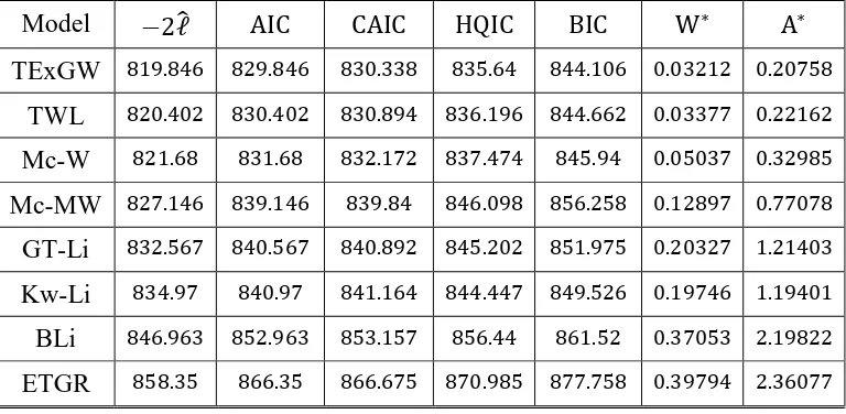
In order to compare the distributions, we consider the goodness-of-fit statistics including the Akaike information criterion ( ), consistent Akaike information criterion ( ), Bayesian information criterion ( ), Hannan-Quinn information criterion ( ), minus twice maximized log-likelihood under the model ( ̂), Anderson-Darling ( ) and Cramér-Von Mises ( ) statistics. The smaller these statistics are, the better the fit is. Upper tail percentiles of the asymptotic distributions of these goodness-of-fit statistics were tabulated in Nichols and Padgett (2006).
Table 2: -
Model ̂
TExGW
TWL
Mc-W
Mc-MW
GT-Li
Kw-Li
BLi
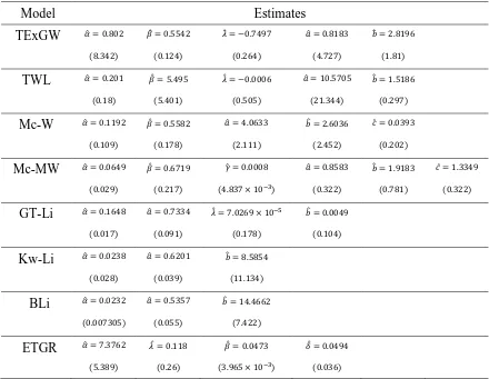
Table 3: MLEs and their standard errors (in parentheses) for cancer data
Model Estimates
TExGW ̂ ̂ ̂ ̂ ̂
( ) ( ) ( ) ( ) ( )
TWL ̂ ̂ ̂ ̂ ̂
( ) ( ) ( ) ( ) ( )
Mc-W ̂ ̂ ̂ ̂ ̂
( ) ( ) ( ) ( ) ( )
Mc-MW ̂ ̂ ̂ ̂ ̂ ̂
( ) ( ) ( ) ( ) ( ) ( )
GT-Li ̂ ̂ ̂ ̂
( ) ( ) ( ) ( )
Kw-Li ̂ ̂ ̂
( ) ( ) ( )
BLi ̂ ̂ ̂
( ) ( ) ( )
ETGR ̂ ̂ ̂ ̂
( ) ( ) ( ) ( )
Table 2 lists the numerical values of ̂, , , , , and for the models fitted. The MLEs and their corresponding standard errors (in parentheses) of the model parameters are given in Table 3.
In Table 2, we compare the fits of the TExGW model with the TWL, Mc-W, Mc-MW, T-Li, Kw-T-Li, BLi and ETGR distributions. The figures in this table indicate that the ExGW distribution has the lowest values for the ̂, , , , , and statistics among the fitted models. Then, the TExGW model could be chosen as the best model. It is clear from Table 2 that the TExGW model provide the best fits to the cancer data.
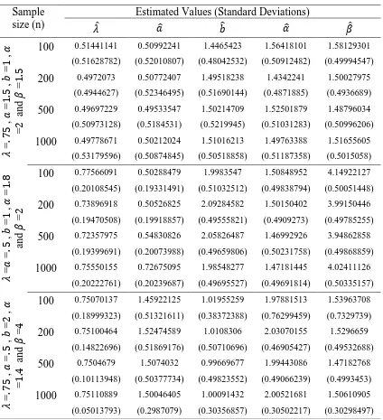
11. Simulation Study
Table 4: MLEs and standard deviations for various parameter values
Sample size (n)
Estimated Values (Standard Deviations)
̂ ̂ ̂ ̂ ̂ = , = , = , = and =
100 0.51441141 0.50992241 1.4465423 1.56418101 1.58129301
(0.51628782) (0.52010807) (0.48042532) (0.50912482) (0.49994547)
200 0.4972073 0.50772407 1.49518238 1.4342241 1.50027975
(0.4944627) (0.52346495) (0.51690144) (0.4871885) (0.4936689)
500 0.49697229 0.49533547 1.50214709 1.52501879 1.48796034 (0.50973128) (0.5184531) (0.5219945) (0.51031283) (0.50996206)
1000 0.49778671 0.50212024 1.51016213 1.49763388 1.51655605 (0.53179596) (0.50874845) (0.50518858) (0.51187358) (0.5015058)
= = , = , = and =
100 0.77566091 0.50288479 1.9983547 1.50848952 4.14922127
(0.20108545) (0.19331491) (0.51032512) (0.49838794) (0.50051448)
200 0.73896918 0.50526825 2.09284582 1.50150402 3.99150446 (0.19470508) (0.19918857) (0.49555821) (0.4909273) (0.49785255)
500 0.72357975 0.54830826 2.05826487 1.46992926 3.94862858 (0.19399691) (0.20073988) (0.49659806) (0.50231758) (0.49868859)
1000 0.75550155 0.72675095 1.98548277 1.47181445 4.02411126 (0.20222761) (0.20239687) (0.49695527) (0.49691814) (0.50335157)
= , = , = , = and =
100 0.75070137 1.45922125 1.01955259 1.97881513 1.53963708 (0.18999323) (0.51321611) (0.38372388) (0.76299459) (0.7329739)
200 0.75100464 1.52474589 1.0108306 2.03070155 1.5296659
(0.14822696) (0.51869176) (0.50710696) (0.46905427) (0.49532688)
500 0.7504679 1.5074032 0.99669677 1.99443086 1.47182768
(0.10113948) (0.50377734) (0.49823552) (0.49066239) (0.4993453)
1000 0.75110889 1.50046405 1.00091432 2.00521681 1.50610905 (0.05013793) (0.2987079) (0.30356857) (0.30502217) (0.30298497)
We repeated the simulation k =100 times and calculated the MLEs and the standard deviations of the parameter estimates. The empirical results are given in Table 4 shows that the estimates are quite stable and are close to the true value of the parameters for these sample sizes.
12. Conclusions
shape parameter. Many well-known models emerge as special cases of the ExG-G family by using special parameter values. Some mathematical properties of the new class including explicit expansions for the ordinary and incomplete moments, quantile and generating functions, mean deviations, entropies, order statistics and probability weighted moments are provided. The model parameters are estimated by the maximum likelihood estimation method and the observed information matrix is determined. We perform a Monte Carlo simulation study to assess the finite sample behavior of the maximum likelihood estimators. We prove empirically by means of an application to a real data set that special cases of the proposed family can give better fits than other models generated from well-known families.
References
1. Afify, A. Z., Hamedani, G. G., Ghosh, I. and Mead, M. E. (2015). The transmuted Marshall-Olkin Fréchet distribution: properties and applications. International Journal of Statistics and Probability, 4, 132-148.
2. Afify, A. Z., Nofal, Z. M. and Butt, N. S. (2014). Transmuted complementary Weibull geometric distribution. Pak.j.stat.oper.res., 10, 435-454.
3. Afify, A. Z., Nofal, Z. M. and Ebraheim, A. N. (2015). Exponentiated transmuted generalized Rayleigh: a new four parameter Rayleigh distribution. Pak.j.stat.oper.res., 11, 115-134.
4. Afify, A. Z., Nofal. Z. M., Cordeiro, G.M., and Yousof, H. M. (2015). The Kumaraswamy transmuted-G family of distributions: properties and applications. Submitted.
5. Afify, A. Z., Nofal, Z. M., Yousof, H. M., El Gebaly, Y. M. and Butt, N. S. (2015). The transmuted Weibull Lomax distribution: properties and application. Pak. J. Stat. Oper. Res., 11, 135-152.
6. Afify, A. Z., Yousof, H. M., and Nadarajah, S. (2015). The beta transmuted-G family of distributions: properties and applications. Submitted.
7. Alexander, C., Cordeiro, G.M., Ortega, E.M.M. and Sarabia, J.M. (2012). Generalized beta generated distributions. Computational Statistics and Data Analysis, 56, 1880-1897.
8. Alizadeh, M., Emadi, M., Doostparast, M., Cordeiro, G. M., Ortega, E. M. M., Pescim, R. R. (2015). A new family of distributions: the Kumaraswamy odd log-logistic, properties and applications. Hacettepa Journal of Mathematics and Statistics, forthcomig.
9. Alizadeh, M., Merovci, F., and Hamedani, G.G. (2015). Generalized transmuted family of distributions: properties and applications. Hacettepa Journal of Mathematics and Statistics, forthcomig.
11. Aryal, G. R., and Tsokos, C. P. (2011). Transmuted Weibull distribution: a generalization of the Weibull probability distribution. European Journal of Pure and Applied Mathematics, 4, 89-102.
12. Cakmakyapan, S. and Kadilar, G. O. (2014). A new customer lifetime duration distribution: the Kumaraswamy Lindley distribution. International Journal of Trade, Economics and Finance, 5, 441-444.
13. Cordeiro, G. M, Alizadeh, M, Tahir, M. H., Mansoor, Bourguignon, M. and Hamedani, G. G. (2015). The beta odd log-logistic generalized family of distributions. Hacettepe Journal of Mathematics and Statistics, forthcoming.
14. Cordeiro, G. M. and de Castro, M. (2011). A new family of generalized distributions. Journal of Statistical Computation and Simulation, 81, 883-898.
15. Cordeiro, G. M., Ortega, E. M. M. and da Cunha, D. C. C. (2013). The exponentiated generalized class of distributions. J. Data Sci., 11, 1-27.
16. Cordeiro, G. M., Hashimoto, E. M., Edwin, E. M. M. Ortega. (2014). The McDonald Weibull model. Statistics: A Journal of Theoretical and Applied Statistics, 48, 256-278.
17. Elbatal, I. and Aryal, G. (2013). On the transmuted additive Weibull distribution. Austrian Journal of Statistics, 42, 117-132.
18. Eugene, N., Lee, C. and Famoye, F. (2002). Beta-normal distribution and its applications, Communications in Statistics-Theory and Methods 31, 497-512.
19. Glänzel, W. (1987). A characterization theorem based on truncated moments and its application to some distribution families. Mathematical Statistics and Probability Theory (Bad Tatzmannsdorf, 1986), B, Reidel, Dordrecht, 75-84.
20. Glänzel, W. (1990). Some consequences of a characterization theorem based on truncated moments. Statistics: A Journal of Theoretical and Applied Statistics, 21, 613-618.
21. Leadbetter, M.R., Lindgren, G. and Rootzén, H. (1987). Extremes and related properties of random sequences and processes. Springer, New York.
22. Khan, M. S., and King, R. (2013). Transmuted modified Weibull distribution: a generalization of the modified Weibull probability distribution. European Journal of Pure and Applied Mathematics, 6, 66-88.
23. Lee, E. T. and Wang J. W. (2003). Statistical methods for survival data analysis. 3rd ed.,Wiley, NewYork.
24. Marshall, A. N. and Olkin, I. (1997). A new method for adding a parameter to a family of distributions with applications to the exponential and Weibull families. Biometrika, 84, 641-652.
25. Mead, M. E. and Afify, A. Z. (2015). On five-parameter Burr XII distribution: properties and applications. South African Statistical Journal, forthcomig.
27. Merovci, F. and Elbatal, I. (2013). The McDonald modified Weibull distribution: properties and applications. arXiv preprint arXiv:1309.2961.
28. Merovci, F. and Sharma, V. K. (2014). The beta Lindley distribution: properties and applications. Journal of Applied Mathematics, 51, 1-10.
29. Nofal, Z. M., Afify, A. Z., Yousof, H. M. and Cordeiro, G. M. (2015). The generalized transmuted-G family of distributions. Communications in Statistics-Theory and Methods, forthcoming.
30. Shaw, W. T. and Buckley, I. R. C. (2007). The alchemy of probability distributions: beyond Gram-Charlier expansions and a skew-kurtotic-normal distribution from a rank transmutation map. Research report.
Appendix A
The elements of the observed matrix ( ) are given below:
∑ ∑ ∑ ∑ ∑ ( ) ( ) ( ) ∑ ∑ ( ) ∑ [ ( ) ( ) ( )] ∑ { [( ) ( )]} ∑ ∑ [ ( ) ] ∑ ( ) ( ) ∑ ( ) ∑ ( ) ∑ [ ( ) ( ) ( )] ∑ ( ) ∑ ∑ ∑ ∑ , -and ∑ ( ) ( ) , ( ( ) ( ) ∑ ( ) ∑ ( ) ∑ ( ) ( ) , ( ( ) ∑ ( ) ∑ ( ) [ ( ) ( ), ( )- ( ) ] ∑ ( ) [ ( ) ( ) ( ) , ( )- ]