Three - Stage Stochastic Multivariate
Stratified Sample Survey
Sanam Haseen
Department of Statistics & Operations Research Aligarh Muslim University, Aligarh, India
Shafiullah
Department of Statistics & Operations Research Aligarh Muslim University, Aligarh, India
Irfan Ali
Department of Statistics & Operations Research Aligarh Muslim University, Aligarh, India [email protected]
Abdul Bari
Department of Statistics & Operations Research Aligarh Muslim University, Aligarh, India
Abstract
In this paper, we have considered the problem of three-stage sample surveys. The problem of a three stage multivariate stratified sample survey has been formulated as a non-linear stochastic programming problem by considering survey cost and the variances as random variables. The stochastic programming problem has been converted into equivalent deterministic form using Chance constraint programming and modified E-model.
Keywords: Three Stage Sample Survey, Stochastic Programming, Modified E-Model, Chance Constraint Programming, Multivariate Stratified Sample Survey.
Introduction
The analysis of two-stage stratified sampling designs is well defined in the sampling literature. In two-stage stratified sampling designs the total population is subdivided into a number of strata and then two-stage stratified sampling procedure is applied for taking the samples. The two- stage stratified sampling designs generally specifies two- stages of selection: primary sampling units (PSUs) at the first stage and sub samples from each
PSUs at second stage as a secondary sampling units (SSUs) units. The methods to obtain the optimum allocations of sampling units to each stage are readily available. Showkat et al. (2011) has used the geometric programming approach in multivariate two-stage sampling design for obtaining optimum sample sizes of each stage.
designs generally specifies three stages of selection: primary sampling units (PSUs) at the first stage, sub samples from each PSUs at second stage as secondary sampling units (SSUs) units and again sub samples from SSUs at third stage as tertiary sampling units (TSUs). For instance, in surveys to estimate crop production in India (Sukhatme, 1947), the village is a convenient sampling unit. Within a village, only some of the fields growing the crop in question are selected, so that the field is a sub-unit. When a field is selected, only certain parts of it are cut for the determination of yield per acre; thus the sub unit itself is sampled. Here we have to find the optimal sample sizes n, m and p for all the three stages with the minimum cost. The problem of optimum allocation in two-stage and three-two-stage sample surveys is described in standard text book on sampling such as W.G. Cochran (1977). Recently Shafiullah et at. (2013) has worked on three-stage sample surveys and applied geometric programming approach for finding optimum sample sizes of each stage.
In many real-life situations the decision makers have to optimize their objectives which they have decided under certain conditions. The parameters on which the decision makers have to optimize their objectives are not always certain. The mathematical programming problem which deals with the theory and methods of the unknown parameters where the variables are considered as random is called stochastic programming problem. Stochastic programming plays very important role for modeling optimization problems. Uncertainty is the root of the stochastic programming. The main target of using stochastic programming is for finding such solution where the feasibility occurs for all data and optimal in some cases. The stochastic programming is discussed by many authors in their text books such as Prékopa (1995), Charnes and Cooper (1959).
The stochastic programming approach is applied by many researchers in the field sample surveys. Some of them are Ali et al. (2011), Khan et al. (2011, 2012), Bakhshi et al.
(2010), Javed et al. (2009), Kozak (2006), Diaz-Garcia and Tapia (2007), Diaz-Garcia and Cortez (2006, 2008) and many more.
In this paper, we have formulated the three-stage sample surveys problem as a stochastic programming problem. In three-stage sample surveys problem, we have considered that sampling variance and stratum costs has normally distributed random variable. The stochastic formulation of the problem has been converted into equivalent deterministic form by using chance constrained programming and modified E- model respectively.
2. Formulation of the problem in Three -Stage Stratified Sample Surveys
The population is considered to be a heterogeneous population; it is turned into a homogeneous population by dividing it into L homogeneous stratum. Let strata have
Let the value in the population of TSU in the SSU in PSU of strata be such that .
Below are some of the usual notations that refer to strata,
Sample mean of TSU that were selected,
̅ ∑
.
Population mean of TSU that were selected,
̅ ∑
.
Sample mean of SSU that were selected,
∑
.
Population mean per SSU that were selected,
∑
.
Sample mean of PSU that were selected,
∑ .
Population mean of PSU that were selected,
∑ .
Required variances are
Sampling variance among PSU means in stratum,
∑ ( ) .
Sampling variance among SSU’s within PSU means in stratum,
( )∑ ∑ ( * .
Sampling variance among TSU’s within SSU means in stratum,
( )∑ ∑ ∑ ( ) .
Population variance among PSU means in stratum
∑ ( + .
Population variance among SSU’s within PSU means in stratum,
( )∑ ∑ ( ) .
Population variance among TSU’s within SSU means in stratum,
An unbiased estimate of population mean, , per TSU may be written as
∑ (∑
,
∑
where ∑
is the relative size of the stratum in terms of the TSU’s.
It is known that for stratified random sampling, WOR, with as the unbiased estimator
of population mean , the sampling variance is given by
( * ∑
(( ) ( ) ( ) )
where are the sample fraction at various stage and its
estimated variance ignoring the fps is given by
̂ ( * ∑
( )
Now, if the travel cost may be ignored, the total cost of survey can be written in the linear form given below
∑( )
where
is the overall cost of sampling. is the fixed cost in survey.
is the cost of obtaining information from the sampled FSU from the stratum. is the cost of obtaining information from the sampled SSU from the stratum. is the cost of obtaining information from the sampled TSU from the stratum.
In practice, is likely to be larger than and is likely to be larger than . Hence, a unit increase in increases the cost much more as compared to a unit increase in similarly, a unit increase in is much more compared to a unit increase in . Thus, the third component of cost function will vary from sample to sample for given .
∑ ( )
∑( )
}
( )
where , and are the sample variances at each stage with characteristic,
Now, let us assume that to be independently normally distributed random variables. Further, sampling variance in the stratum are also random variables.
∑ ( )
( )
[ ∑( )
] ( )
( ) ( )}
( )
4. Solution Using Modified E-technique
In objective function of Eq. 2 (i) are considered random variables with asymptotic normal distribution. Consider the random variable defined as (See Melaku, 1986)
∑ ( +
which has an asymptotic normal distribution with mean
( )
and
( )
( ) ( ( ) )
where is the fourth central moment and it is computed as
∑ ( +
Observe that, ( + ;
where and ( + in terms of probability.
Consider the random variable defined as
( )∑ ∑ ( )
which has an asymptotic normal distribution with mean ( ) and ( ) given by ( )
( ) and
( )
( ) ( ( ) )
where is the fourth central moment and it is computed as
( )∑ ( )
Observe that, ( ) ;
where and ( ) in terms of probability.
Again, consider the random variable defined as
( )∑ ∑ ∑ ( )
which has an asymptotic normal distribution with mean ( ) and variance ( ) ( )
( )
and ( ) ( ) ( ( ) )
where is the fourth central moment and it is computed as
( )∑ ( )
Observe that, ( ) ;
where and ( ) in terms of probability.
Now, modified E-model technique (Garcia-2007) is applied, so that the equivalent deterministic objective function of NLPP (2) can be written as
( )
(∑ ( *
Now, (∑ ( ** ∑ ( ( ) ( ) ( ))
∑ ( ( ) ( ) ( ) * ∑ (
( )
( )
( )*
Also, (∑ ( ** ∑ ( ( ) ( ) ( ))
∑ ( ( ) ( ) ( ) * ∑ ( ( ) ( ) ( ) *
where ( ) ( ) ( )
The equivalent deterministic form of Eq. 2(i) can be obtained by using modified E-model as
(∑ (
( )
( )
( )*
*
(√∑ ( ( ) ( ) ( ) *) (3)
3. Solution Using Chance Constraint Programming
The costs in the constraint are assumed to be normally distributive random variables.
(∑ ) ∑ ( )
∑ ( ) (∑ ) ∑ ( )
∑ ( ) (∑ ) ∑ ( )
∑ ( ) (∑ ) ∑ ( )
∑ ( )
(∑ ) ∑ ( )
∑ ( )
(∑ ) ∑ ( )
∑ ( )
Finally, from Eq. (4), (6) and (8) mean of objective function with random cost will be ( )
∑ (
) ( )
and variance from Eq. (5), (7) and (9) with random cost is ( )
∑ (
Since, are unknown and therefore they are replaced by
their estimators. The estimator of ( ) is ̂( )
∑ (
) ( )
The estimator of (∑ ( ( ))) is ̂( )
∑ (
) ( )
where ∑ ( ).
Again, ( ̂ ( ) ) ( ̂ ( ) ) also imply
(
̂ ( ) ( ̂( ))
√ ( ̂( ))
( ̂( ))
√ ( ̂( )) )
which in simplified form is given by
( ̂ ( ) )
(
( ̂( ))
√ ( ̂( )) )
where ( ( ̂( ))
√ ( ̂( )) ) is a standard normal variate (SNV) with mean zero and variance one.
Now, ( ) represents the cumulative density function of the SNV evaluated at z. If represents the value of SNV at which ( ) , then the constraint be stated as
(
( ̂( ))
√ ( ̂( )) )
( )
This inequality will satisfy only if ( ̂( ))
√ ( ̂( ))
or ( ̂( )) √ ( ̂( ))
∑( )
√∑( )
( )
Thus finally, the allocation problem will be using assumptions made for (see Melaku 1968) and using modified E-model (see Garcia 2007) the NLPP (3) will be formulated as
(∑ ( ( ) ( ) ( )* * (√∑ ( ( ) ( ) ( ) *) ∑ √∑ } ( ) Lexicographic Method
To solve the converted deterministic NLPP using lexicographic goal programming approach the with r characteristics arranged in lexicographic order of importance, at the first stage of the solution the NLPP with has to be obtained. Let be the optimal value of the objective function and is such that .
At the second stage of the solution the NLPP to be solved is given by
(∑ ( ( ) ( ) ( )* * (√∑ ( ( ) ( ) ( ) *) (∑ ( ( ) ( ) ( )* * (√∑ ( ( ) ( ) ( ) *) ∑ √∑
Successively solving the problem at each stage, the NLPP at stage will be given as
(∑ ( ( ) ( ) ( )* * (√∑ ( ( ) ( ) ( ) *) (∑ ( ( ) ( ) ( )* * (√∑ ( ( ) ( ) ( ) *) ∑ √∑
Other Allocation Methods
A Comparative Study
1. Proportional allocation
2. Cochran’s Allocation
The compromise criterion of Cochran’s allocation is to average the individual optimum allocations of that are solutions to the NLPP for all the p characteristics separately.
3. Minimizing Weighted Sum of Variances
Khan et al. (2003) conjectured that
∑
∑ ∑ ∑
( ) ∑
∑ (∑ ( )
+
∑ ( )
where, ∑
∑
∑
4. Sukhatme’s Allocation
Sukhatme et al. [16] obtained the compromise allocation by minimizing the sum of the variances for the p characteristics under linear cost constraints. The NLPP for this allocation is given as
∑ (∑ (
( )
( )
( )*
* (√∑ ( ( ) ( ) ( ) *)
∑ √∑
Simulation Study
To illustrate the theory developed in previous section a simulation study has been done. Considering the population to posses two characteristics, randomized data with normal probabilities have been generated at each stage with total population being divided into four stratum. The data for simulation of three stage sampling is obtained through R-Software.
strata. The normal random variables are regenerated with different mean and standard deviation for second characteristic.
Similarly, different populations at each stage are generated and regenerated for second characteristic for pre-assumed means and variances. The required data generated through the R-software for characteristic one and two are shown in table 1 and 2 respectively.
Table 1: Characteristic one i.e.
1 28 120 240 101.4907 149.3986 338.1822 16744.84 76925.87 328265.00 2 35 88 238 127.7659 144.2444 420.0881 30352.46 58804.94 454358.00 3 25 116 256 89.4826 131.6389 434.8655 21610.17 57372.1 603104.40 4 32 96 266 106.1326 114.8018 422.8810 23220.17 39431.28 590399.00
Table 2: Characteristic two i.e.
1 28 120 240 75.0717 99.2154 198.4202 10692.33 26751.71 109388.30
2 35 88 238 78.6746 88.9380 166.7440 12815.83 31685.18 101540.80
3 25 116 256 37.6336 101.4011 152.4509 3076.868 23863.5 78502.63 4 32 96 266 62.6065 102.4223 188.7107 10507.18 27047.83 128872.50
The per unit cost for measurement in various strata are independently normally distributed with assumed means and variances as shown in table below
( ) ( ) ( )
3 2 1 0.75 0.50 0.25
4 3 1 1.00 0.75 0.25
5 4 1 1.25 1.00 0.25
6 5 1 1.50 1.25 0.25
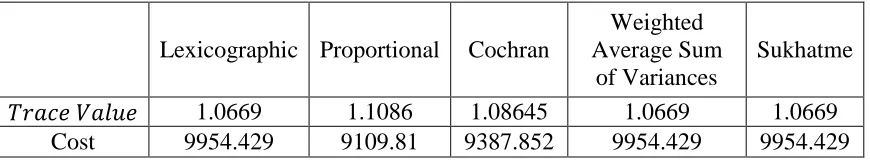
Results
Trace Values and Cost from different methods are given in the form of table below
Lexicographic Proportional Cochran
Weighted Average Sum
of Variances
Sukhatme
1.0669 1.1086 1.08645 1.0669 1.0669
Cost 9954.429 9109.81 9387.852 9954.429 9954.429
Conclusions
three-stage multivariate stratified sample surveys is converted into equivalent deterministic form by using Chance constraint programming and modified E-model. Furthermore the researchers can use these formulations for obtaining optimum allocation for three-stage sample surveys whenever their costs are needed to be optimized with a limitation on variance.
References
1. Ali, I, Raghav, Y.S. and Bari, A. (2011). Compromise allocation in multivariate stratified surveys with stochastic quadratic cost function, Journal of Statistical Computation and Simulation, 83(5), pp. 960-974 (Taylor & Francis,
DOI:10.1080/00949655.2011.643890).
2. Bakhshi, Z.H. Khan, M.F. and Ahmad, Q.S. (2010). Optimal sample numbers in multivariate stratified sampling with a probabilistic cost constraint, Int. J. Math. Appl. Statist. 1(2), pp. 111–120.
3. Charnes, A. and Cooper, W.W. (1959). Chance constrained programming,
Management Science 5, pp. 73–79.
4. Cochran, W.G. (1977): Sampling Techniques, 3rd ed., Wiley, New York.
5. Díaz-García J. A. and M.M. Garay Tapia, (2007). Optimum allocation in stratified surveys: Stochastic programming, Comput. Statist. Data Anal. 51, pp. 3016–3026. 6. Díaz-García J.A. and Cortez, L.U. (2006). Optimum allocation in multivariate stratified sampling: Multiobjective Programming. Comunicación Técnica No. I-06–07/28–03–2006 (PE/CIMAT), México.
7. Díaz-García, J.A. and Cortez, L.U. (2008). Multi-objective Optimisation for optimum allocation in multivariate stratified sampling. Surv. Methodol. 34(2), 215–222
8. Ignizio, J.P., Goal Programming and Extensions, Lexington, Mass: Health, Lexinton Books, Lexington, MA, 1976.
9. Ijiri, Y., Management goals and Accounting for control, North Holland, Armsterdam, 1965.
10. Javed S., Bakhshi Z.H. and Khalid M.M. (2009). Optimum allocation in stratified sampling with random costs, Int. Rev. Pure Appl. Math. 5(2), pp. 363–370.
11. Khan, M.F., Ali, I, Raghav, Y.S. and Bari, A. (2012). Allocation in multivariate stratified surveys with non- linear random cost function, American Journal of Operations Research (USA), 2(1), pp. 122-125.
12. Khan, M.F., Ali, I. and Ahmad, Q.S. (2011). Chebyshev Approximate Solution to Allocation Problem in Multiple Objective Surveys with Random Costs 1, pp. 247-251 (doi:10.4236/ajcm.2011.14029).
13. Kozak, M. (2006). On Sample Allocation in Multivariate Surveys,
Communications in Statistics - Simulation and Computation, 35:4, 901-910. 14. Lee, S.N., Goal Programming for Decision Analysis, Aurebach, Philadelphia,
15. Maqbool, S., Mir, A. H. and Mir, S. A. (2011). Geometric Programming Approach to Optimum Allocation in Multivariate Two-Stage Sampling Design. Electronic Journal of Applied Statistical Analysis, 4(1), pp. 71 – 82
16. Melaku, A., (1986). Asymptotic normality of the optimal allocation in multivariate stratified random sampling. Indian J. Statist. 48 (Series B), 224–232.
17. Pandit, S.N.N. and Srinivas, K. (1962). A Lexisearch algorithm for traveling Salesman problem, IEEE, 2521-2527.
18. Prékopa, A. (1995). Stochastic Programming, Series in Mathematics and its Applications, Kluwer Academic Publishers, Dordrecht, The Netherlands.
19. Rao, S.S., (1979). Optimization Theory and Applications. Wiley Eastern Limited. 20. Shafiullah, Ali, I. and Bari, A. (2013): Geometric Programming Approach in
Three – Stage Sampling Design, International Journal of Scientific & Engineering Research (France), 4(6), pp. 2229-5518.