A novel biclustering algorithm of binary microarray data: BiBinCons and BiBinAlter

(1)

R E S E A R C H

Open Access

A novel biclustering algorithm of binary

microarray data: BiBinCons and BiBinAlter

Haifa Ben Saber

1*

and Mourad Elloumi

1,2

*Correspondence: [email protected] 1Latice laboratory, ENSIT, Tunis Time université, Tunis, Tunisia Full list of author information is available at the end of the article

Abstract

The biclustering of microarray data has been the subject of a large research. No one of the existing biclustering algorithms is perfect. The construction of biologically

significant groups of biclusters for large microarray data is still a problem that requires a continuous work. Biological validation of biclusters of microarray data is one of the most important open issues. So far, there are no general guidelines in the literature on how to validate biologically extracted biclusters. In this paper, we develop two biclustering algorithms of binary microarray data, adopting theIterative Row and Column Clustering Combination(IRCCC) approach, calledBiBinConsandBiBinAlter. However, theBiBinAlteralgorithm is an improvement ofBiBinCons. On the other hand, BiBinAlterdiffers fromBiBinConsby the use of theEvalStabandIndHomogevaluation functions in addition to theCroBinone (Bioinformatics 20:1993–2003, 2004).BiBinAlter can extracts biclusters of good quality with betterp-values.

Keywords: Biclustering, Algorithm, Evaluation function, Microarray data analysis

Introduction

DNA microarray technology is a revolutionary tool enabling the measurement of ex-pression levels of thousands of genes in a single experiment under diverse experimental conditions. This technology allows us to obtain big raw data that can provide a wealth of information on the concerned genes. It proved to be a valuable tool for many bio-logical and medical applications. Indeed, microarray data analysis is a crucial step for these applications in order to extract pertinent biological knowledge embedded in these large masses of data. However, the extraction process of this knowledge is far from being trivial. From here comes the necessity to adoptdata miningtechniques. Many of these techniques were applied to these data in order to extract pertinent biological knowledge. Among the techniques that are used, we mention those ofclustering[1]. Indeed, by mak-ing aclustering, we consider that all the genes of a group can have a similar behavior under all the conditions. However, there are genes that have a similar behavior only under a subset of conditions. Hence, clustering is too simplistic to detect such cases [1]. Another more interesting technique, calledbiclustering[2], allows to identify groups of genes that have a similar behavior only under a subset of conditions.

In this paper, we develop new biclustering algorithms of microarray data. These data are usually coded by a data matrixM(I,J), where theithrow,i∈I= {1, 2,. . .,n}, represents theithgene, thejthcolumn,j∈J= {1, 2,. . .,m}, represents thejthcondition and the cell M[i,j] represents the expression level of theithgene under thejthcondition.

(2)

The main objective is then to identify groups of genes that are coherent under groups of conditions, these groups are calledbiclusters. Genes belonging to the same bicluster have close biological functions. Let’s note that, in its general form, the biclustering problem is NP-hard [2].

The rest of this chapter is organized as follow: In the second section, we introduce some preliminaries. In the third section, we present theBiBinCons algorithm. In the fourth section, we present theBiBinAlter algorithm. In the fifth section, we present an illustrative example and an experimental study. Finally, we present the conclusion of this paper.

Preliminaries

As we said in the introduction, the biclustering algorithms that we present in this paper are based onCroBin [1] function for the evaluation of a group of biclusters. So, let’s present some preliminaries related to this function. LetI= {1, 2,. . .,n}be a set of indices ofngenes,J= {1, 2,. . .,m}be a set of indices ofmconditions andMb(I,J)=

mb_ij,i∈ I andj∈J, be a binary data matrix associated withIandJ. The biclustering problem of a binary microarray data can be formulated as a minimization of the criterionW(z,w,a):

W(z,w,a)=

a

k=1 m

l=1

i∈zk

j∈wl

mb_ij−akl. (2.1)

where

z = {z,z2,. . .,zg}is the matrix defined as a partition ofIintogclusters, i.e. ziis the cluster number of theithrow ofMb(I,J).

w= {w1,w2,. . .,wh} is the matrix defined as a partition ofJintohclusters, i.e.wiis the cluster number of thejthcolumn ofMb(I,J)..whe

a=(akl) is asummary matrixofMb(I,J), it is a binaryg×hmatrix wherek(resp.l) is the number of clusters on rows (resp. columns) andakl is defined by themij’s satisfaying the following condition:

zikwjl=1 (2.2)

where

zik =1 if theithrow ofMb(I,J)belongs to thekthcluster ofIotherwisezik=0.

wjl=1 if thejthcolumn ofMb(I,J)belongs to thelthcluster ofJotherwisewjl=0.

By using Eq. (2.2), Eq. (2.1) can be reformulated as follows:

W(z,w,a)=

i,j,k,l

zikwjlmbij−akl (2.3)

By adopting the IRCCC approach, we can make biclustering by minimizingW(z,w,a) defined by Eq. (2.3) and by fixing eitherworz:

• Ifw is fixed, the minimization is given by:

W(z,a|w)=

i,k,l

(3)

whereu_il=_j_∈_w

lmij=

jwjlmij, i,j,k,l

z_ikw_jlmb

ij−akl=

i,k

z_ik

j,l

w_jlmb

ij−akl=

i,k

zik

l

|uil−(|wl| ×akl)|,u is a matrix of size|I| ×l.

• Ifz is fixed, the minimization is given by:

W(w,a|z)=

i,k,l

w_jl|v_jl−(|z_k| ×a_kl)| (2.5)

wherevkj=i∈zkm b ij=

izikmij, i,j,k,l

zikwjlmbij−akl= j,l

wjl i,k

zikmbij−akl=

i,k

zik l

|vkj−(|zk| ×akl)|,v is a matrix of sizek× |J|.

Remark.A colored block in the binary matrixMb(I,J)will be represented by a col-ored cell in the summary matrixA, where each colored cell contains the majority binary value in the corresponding colored block, e.g, if the majority of cells in a block inMb(I,J) contains 1 then the corresponding cell inAcontains also 1.

Example.This example shows a binary data matrixMb(I,J)and the corresponding cell in the summary matrixA.

A=(0, 0; 1, 1; 1, 1), i.e.,a11=0,a12=0;a21=1,a22=1;a31=1,a32=1.

In the section ‘FIRST IRCCC Algorithm: BiBinCons’, we develop two IRCCC algorithms of biclustering of binary microarray data, called respectivelyBiBinConsand BiBinAlter.

FIRST IRCCC Algorithm:BiBinCons

Our biclustering algorithm, BiBinCons receives as input a binary matrix Mb(I,J) and gives as output (zopt,wopt,Aopt), wherezopt andwoptare respectively the final clustering of rows and columns ofMb(I,J), andAoptis the summary matrix related tozoptandwopt. To describe more formally our biclustering algorithm,BiBinCons, we use the following notations:

z0: initial clustering of rows ofMb(I,J)

w0: initial clustering of columns ofMb(I,J),

A0: initial summary matrix related toz0andw0

zc: current clustering of rows ofMb(I,J)

wc: current clustering of columns ofMb(I,J),

(4)

Ac: current summary matrix related tozcandwc

zopt: final clustering of rows ofMb(I,J)

wopt: final clustering of columns ofMb(I,J)

Aopt: final summary matrix related tozoptandwopt

A_c: intermediate current summary matrix.

Algorithm 1BiBinCons input :Mb(I,J)

output :(zopt,wopt,Aopt)

Compute (z0,w0,A0) thanks to the initialization step ofBiMaxalgorithm Preli´c et al. [3], // Initialization step :

c:=1

while(zc,wc−1,A_c)=(zc−1,wc−1,Ac−1)do////////////// Clustering of rows

////Compute (zc,wc−1,A_c) starting from (zc−1,wc−1,Ac−1), by using Eq. 2.4 end while

(zc−1,wc−1,Ac−1):=(zc,wc−1,A_c)

while(zc,wc,Ac))=(zc−1,wc−1,Ac−1)do////////////// Clustering of columns

////Compute (zc,wc,Ac) starting from (zc,wc−1,Ac), by using Eq. 2.5

end while

(zopt,wopt,Aopt):=(zc,wc,Ac) return(zopt,wopt,Aopt)

Second IRCCC Algorithm:BiBinAlter

Our biclustering algorithm,BiBinAlterreceives as input a binary matrixMb(I,J)and gives as output (zopt,wopt,Aopt), wherezoptandwoptare respectively the final clustering of rows and columns ofMb(I,J), andAopt is the summary matrix related tozopt andwopt. By adoptingBiBinAlter, we propose the use of functions defined:

EvalStabcrepresents the frequency of 0’s in the current group of biclusters at thecth iteration. It is defined as follows:

EvalStab=

k,l

|akl−(|zk| × |wl|)|

|z_k||w_l| (4.1)

IndHomogcrepresents the tradeoff between the number of mixed biclusters (containing both 0’s and 1’s) and the total number of biclusters at thecthiteration. It is defined as follows:

IndHomog= MixedBic

AllBic (4.2)

To describe more formally our biclustering algorithm,iBinAlter, we have used the same notations like previous algorithm besides of these notations:

EvalStabc,IndHomogc

: couple to present the frequency of 0’s in the current group of biclusters at thecthiteration and the tradeoff between the number of mixed biclusters (containing both 0’s and 1’s) and the total number of biclusters at thecthiteration.

EvalStabc−1,IndHomogc−1

(5)

EvalStab₍_c₋₁₎,IndHomog₍_c₋₁₎: couple to present the frequency of 0’s in the group of biclusters at the intermidate(c−1)thiteration and the tradeoff between the number of mixed biclusters (containing both 0’s and 1’s) and the total number of biclusters at the intermidate(c−1)thiteration.

Algorithm 2BiBinAlter input :Mb(I,J)

output :(zopt,wopt,Aopt)

//Initialization step : compute (z0,w0,A0)

////

//Biclustering step :

while(((zc,wc,Ac)=(zc−1,wc−1,Ac−1))and(EvalStabc,IndHomogc)

=(EvalStabc−1,IndHomogc−1)))or(((zc,wc,Ac)=(zc,wc−1,Ac))and((EvalStabc,IndHomogc) =(EvalStab_(c₋₁₎,IndHomog_(c₋₁₎))do

Compute(zc,wc−1,A_c) starting from (zc−1,wc−1,Ac−1), by using Eq. 2.4 //Ais an intermediate summary matrix ;

Compute(EvalStab_c,IndHomog_c), by using Eqs. 4.1 and 4.2 Compute (zc,wc,Ac) starting from (zc,wc−1,A_c), by using Eq. 2.5 Compute(EvalStabc,IndHomogc), by using Eqs. 4.1 and 4.2

end while

(zopt,wopt,Aopt):=(zc,wc,Ac) return (zopt,wopt,Aopt)

Illustrative example

Let’s apply theBiBinAlteralgorithm on the following binary matrixMb(I,J):

C1 C2 C3 C4 C5

G1 1 1 0 1 0

G2 0 0 1 0 1

G3 1 1 0 1 0

G4 0 0 1 0 1

M_b(I,J)

• Initialization step

First, we initialize the rows and columns thanks to the initialization step ofBiMax algorithm Preli´c [3] and we compute (z0,w0,A0), we obtain:

(6)

A colored block in the binary matrixMb(I,J)will be represented by a colored cell in the summary matrixA0, where each colored cell contains the majority binary value in the corresponding colored block, e.g, if the majority of cells in a block inMb(I,J)contains 1 then the corresponding cell inA0contains also 1.

• Biclustering step:

Iteration 1:c=1 We compute (z1,w0,A

1) starting from (z0,w0,A0) by using Eq. 2.4, we obtain:

z1,w0,A 1

=((1, 3, 2, 1),(1, 1, 2, 2, 2),(1, 1; 1, 0; 0, 1))

We compute(EvalStab₁,IndHomog₁)by using Eq. 4.3, we obtain:

EvalStab₁,IndHomog₁

= 2,2 3

We compute (z1,w1,A1) starting from (z1,w0,A

1), by using Eq. 2.4, we obtain: (z1,w1,A1)=((1, 3, 2, 1),(2, 2, 1, 2, 1),(1, 1; 1, 0; 0, 1))

We compute(EvalStab1,IndHomog1), by using Eq. 4.3, we obtain:

EvalStab1,IndHomog1

= 1,2 6

Since we have

(((zc,wc,Ac)=(zc−1,wc−1,Ac−1))and(EvalStabc,IndHomogc) =(EvalStabc−1,IndHomogc−1)

and

(((zc,wc,Ac)=(zc,wc−1,A

c))and((EvalStabc,IndHomogc) =(EvalStab₍_c₋₁₎,IndHomog₍_c₋₁₎))

we make another iteration Iteration 2:c=2 We compute (z2,w1,A

2) starting from (z1,w1,A1), by using Eq. 2.4, we obtain:

z2,w1,A 2

=((2, 1, 2, 3),(2, 2, 1, 2, 1),(0, 1; 1, 0, 0, 1))

We compute(EvalStab₂,IndHomog₂), by using Eq. 4.3, we obtain:

EvalStab₂,IndHomog₂= 0,0 6

(7)

EvalStab2,IndHomog2= 0,0 6

Since we have

(((zc,wc,Ac)=(zc−1,wc−1,Ac−1))and(EvalStabc,IndHomogc) =(EvalStabc−1,IndHomogc−1)))

and

(((zc,wc,Ac)=(zc,wc−1,A

c))and ((EvalStabc,IndHomogc) =(EvalStab₍_c₋₁₎,IndHomog₍_c₋₁₎))

we make another iteration Iteration 3:c=3

We compute (z3,w2,A₃) starting from(z2,w2,A2), by using Eq. 2.4, we obtain:

z3,w2,A 3

=((1, 1, 1, 1),(2, 2, 1, 2, 1),(1, 1)) (4.3)

We compute(EvalStab₃,IndHomog₃), by using Eq. 4.3, we obtain:

EvalStab₃,IndHomog₃=(1, 1)

Since we have

(8)

(((zc,wc,Ac)=(zc,wc−1,A

we make another iteration Iteration 4:c=4 We compute (z4,w3,A

4) starting from(z3,w3,A3), by using Eq. 2.4, we obtain:

z4,w3,A 4

=((1, 2, 1, 2),(2, 2, 1, 2, 1),(1, 0; 0, 1))

We compute

EvalStab₄,IndHomog₄

, by using Eq. 4.3, we obtain:

EvalStab₄,IndHomog₄= 0,0 4

4), by using Eq. 2.4, we obtain:

(z4,w4,A4)=((1, 2, 1, 2),(1, 1, 1, 1, 1),(1; 0))

We computeEvalStab4_,_IndHomog4_{, by using Eq. 4.3, we obtain:}

EvalStab4,IndHomog4=(1, 1)

Since we have

and

(((zc,wc,Ac)=(zc,wc−1,A

we make another iteration Iteration 5:c=5

We compute (z5,w4,A₅) starting from(z4,w4,A4), by using Eq. 2.4, we obtain:

z5,w4,A 5

(9)

We compute(EvalStab₅,IndHomog₅), by using Eq. 4.3, we obtain:

EvalStab₅,IndHomog₅

=(1, 1)

5), by using Eq. 2.4, we obtain:

(z5,w5,A5)=((1, 2, 1, 2),(1, 1, 2, 1, 2),(1, 0; 0, 1))

We have (EvalStab₄,IndHomog₄) = (EvalStab5,IndHomog5)) and (z5,w5,A5) = (z4,w3,A

4). Since we have

(((zc,wc,Ac)=(zc,wc−1,A

we stop the loop.

Then, we obtain (zopt,wopt,Aopt) = (z5,w5,A5). Biclusters that contain only 0’s will not be considered because they represent genes that are not expressed under the related conditions. Finally, (zopt,wopt,Aopt) can be represented inMb(I,J)as follows:

Results for synthetic datasets

(10)

obtained by a selection of known algorithms cited in the literature. We conducted experi-ments on synthetic and real datasets of microarrays. The idea behind testing on synthetic datasets is to investigate the ability of our algorithms to extract different types of biclus-ters. However, on real datasets, we seek to assess the degree of response of our algorithms for statistical and biological criteria.

Synthetic microarray datasets and comparaison criteria

By adopting the strategy and data described in [1], we have experimented our algorithms on synthetic datasets by operarting as follows: First, we choose the number of biclusters, 3 clusters on rows (g=3 ) and 2 clusters on columns (m=2). Second, we use theLatent Bernoulli Mixture(LBM) model [1] to generate binary matrices (mixtures) by considering:

(a) Overlapping biclusters (overlapping rate=5 %(well separated), 15 % (fairly separated) and 25 % (poorly separated)).

(b ) Different data sizes (matrix size=50×30(small),100×60(medium) and 200×120(large)).

Similar to [4], we use two indices,RecoveryandRelevance, to evaluate our biclustering algorithms: LetB1be a group of true implemented biclusters in a binary data matrixMb andB2be a group of output biclusters of a biclustering algorithm,Relevancereflects to what extentB2is similar toB1, whileRecoveryquantifies how well each bicluster inB1is recovered byB2[3]:

Recovery=Overlap(B2,B1) (6.1)

Relevance=Overlap(B1,B2) (6.2)

where:

Overlap(B1,B2)= 1 |B1|

(I1,J1)∈B1

max (I2,J2)∈B2

|I1∩I2||J1∩J2| |I1∪I2||J1∪J2|

(6.3)

We use also two other indices cited in [2],

Shared= Scb Totsize

100 (6.4)

NotShared= Sncb Totsize

100 (6.5)

where

Scb is the volume of correctly extracted biclusters, Totsize is the total volume of implemented biclusters andSNCBis the volume of not correctly extracted biclusters.

TheSharedindex (resp. NotShared) represents the percentage of correctly (resp. not correctly) extracted biclusters with respect to all implemented biclusters in the data ma-trix. Indeed, when the Shared value is equal to 100 %, the algorithm extracts all the implemented biclusters. When the value ofNotSharedis 0 %, the algorithm extracts no cell outside the implemented biclusters.

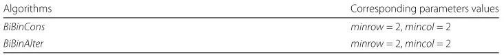
Table 1Corresponding parameters values of our algorithms

Algorithms Corresponding parameters values

BiBinCons minrow= 2,mincol= 2

(11)

Table 2Values ofSharedandNotSharedfor non overlapping biclusters

Algorithms Shared NotShared

CC 18.21 % 36.57 %

OPSM 46.39 % 74.42 %

ISA 39.38 % 5.31 %

BiMax 58.18 % 21.39 %

BiBinCons 88 % 12 %

BiBinAlter 100 % 37.03 %

Experimental protocol

We have compared our algorithms to CC Cheng and Wee-Chung [2], OPSM Ben-Dor and Yakhini [5], ISA Ihmels et al. [4] and BiMax Kaiser and Leisch [6]. These algorithms were implemented in theBIClustering Analysis Toolbox(Bicat) platform. After several simulations, the parameters of our algorithms were set as listed in Table 1. Indeed, at each simulation, we set a parameter and we vary the other and vice inverse. Finally, we keep the parameters which give the nearest implemented biclusters in the starting template.

For CC, OPSM, ISA and BiMax algorithms, we keep the value of the default parame-ters values. Indeed, these values give biclusparame-ters of reasonable quality. We have adopted Shared, NotShared, RecoveryandRelevanceas comparaison criteria. Table 2 shows the best biclusters extracted by each algorithm:

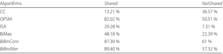
As we can notice in Table 2, for the generated binary matrices, the best values ofShared andNotSharedfor non overlapping biclusters were obtained by theBiBinAlteralgorithm. Indeed, to get a solutionBopt, the combination between two biclusters provides addi-tional volume for the conditions. This reasonnable addiaddi-tional volume is generated by a successive comparaisons betweenPmax and the other polynoms ofL, and we locate the polynomPuncomonthat has the lowest numberρof uncommon terms withPmax. In fact, the interesting resulat is obtained because of we keep only the conditions that have not been removed by the pretreatment process. Besides, the extracted bicluster from the current matrixMb(I,J)is removed ans we set the cells ofMb(I,J), representing the new bicluster, to 0. Table 3 shows the best biclusters extracted by each algorithm. As we can notice in Table 3, for the generated binary matrices, the best values ofShared andNotSharedfor overlapping biclusters were also obtained by theBiBinAlteralgorithm. We can explain this as follows: BiBinAlterresults covers most of the implemented bi-clusters. Table 4 presents the number of biclusters obtained bu our algorithms on real datastes.

Results of our algorithms on real datasets

In this section, we evaluate our algorithms on real microarray datasets.

Table 3Values ofSharedandNotSharedfor overlapping biclusters

Algorithms Shared NotShared

CC 13.21 % 36.57 %

OPSM 82.02 % 50.51 %

ISA 29.28 % 7.31 %

BiMax 48.18 % 22.39 %

BiBinCons 87.30 % 61 %

(12)

Table 4Number of biclusters obtained by our algorithms on real datasets

Algorithms Yeast cell cycle Human B-cell Lymphoma

EnumLat 883 1921

DecBinBicluster 708 1720

BiBinCons 529 1900

BiBinAlter 881 1769

RefineBicluster 708 1700

Real microarray datasets

We have used two real microarray datasets: The Yeast cell cycle dataset which has been described and then pretreated in [1]. It contains the expression of 2884 genes in 17 terms ans the Human B-cell Lymphoma dataset which has been described by Alizadeh et al. [1], it contains 4026 genes and 96 conditions. These datasets are used frequently in the literature by biclustering algorithms.

Experimental protocol

The first experiments concern the statistical validation. It enables to calculate the cov-erage forYeast cell cycleandHuman B-cell Lymphomadatasets and thep-value adjusted forHuman B-cell Lymphomadatasets. The second experiments was applied toYeast cell cyclein order to study the biological significance of extracted biclusters.

Statistical validation

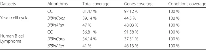
In order to validate statistically our algorithms on these real datasets, we evaluate the performance ofBiBinConsandBibinAlter. We calculate the total number of cells covered by the biclusters. To do this, we have processed as in [2], and we have compared the results of our algorithms to those reported in [2]. In the literature, the coverage test was performed on Yeast cell cycleandHuman B-cell Lymphoma datasets. This test is not applied toRefineBiclusteralgorithm because it is only a refinement algorithm.

Table 5 reports the percentage ofCoverageon the different algorithms for Yeast cell cycleandHuman B-cell Lymphomadatasets. We note that most algorithms have more or less close rates. For example, for theYeast cell cycledatase,BiBinConshas the lowest per-formance. This is explained by the fact thatBiBinConsextracts thousands of small sized biclusters. The CC algorithm extracts biclusters with random values. Thus, CC prohibits the genes/conditions already discovered to be selected in the next search process. This type of mask leads to a high coverage and preventing the discovery of large biclusters.

Biological validation

To evaluate biologically extracted biclusters, we use the web tool GOTermFinder. To do this, we present the most significant shared biclusters. In this section, we evaluate

Table 5Values ofCoverageforYeast cell cycleandHuman B-cell Lymphomadatasets

Datasets Algorithms Total coverage Genes coverage Conditions coverage

Yeast celll cycle

CC 81.47 % 97.12 % 100 %

BiBinCons 39.14 % 44.5 % 100 %

BiBinAlter 47 % 48,03 % 100 %

Human B-cell Lymphoma

CC 36.81 % 91.58 % 100 %

BiBinCons 34.14 % 37.51 % 100 %

(13)

and

E

lloumi

BioData

M

ining

(2015) 8:38

Page

13

of

14

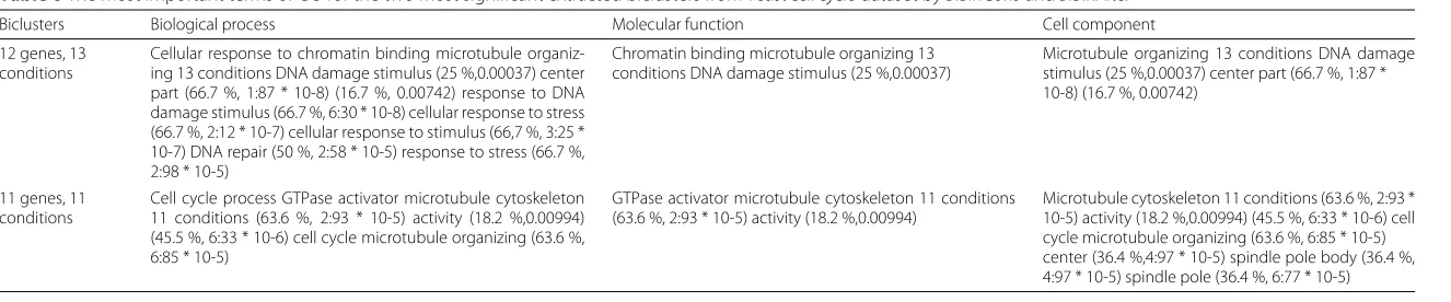
Table 6The most important terms of GO for the two most significant extracted biclusters fromYeast cell cycledataset byBiBinConsandBiBinAlter

Biclusters Biological process Molecular function Cell component

12 genes, 13 conditions

Cellular response to chromatin binding microtubule organiz-ing 13 conditions DNA damage stimulus (25 %,0.00037) center part (66.7 %, 1:87 * 10-8) (16.7 %, 0.00742) response to DNA damage stimulus (66.7 %, 6:30 * 10-8) cellular response to stress (66.7 %, 2:12 * 10-7) cellular response to stimulus (66,7 %, 3:25 * 10-7) DNA repair (50 %, 2:58 * 10-5) response to stress (66.7 %, 2:98 * 10-5)

Chromatin binding microtubule organizing 13 conditions DNA damage stimulus (25 %,0.00037)

Microtubule organizing 13 conditions DNA damage stimulus (25 %,0.00037) center part (66.7 %, 1:87 * 10-8) (16.7 %, 0.00742)

11 genes, 11 conditions

Cell cycle process GTPase activator microtubule cytoskeleton 11 conditions (63.6 %, 2:93 * 10-5) activity (18.2 %,0.00994) (45.5 %, 6:33 * 10-6) cell cycle microtubule organizing (63.6 %, 6:85 * 10-5)

GTPase activator microtubule cytoskeleton 11 conditions (63.6 %, 2:93 * 10-5) activity (18.2 %,0.00994)

(14)

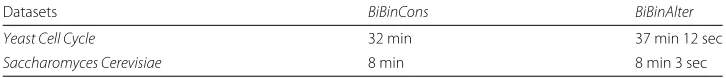
Table 7Computing time of our algorithms

Datasets BiBinCons BiBinAlter

Yeast Cell Cycle 32 min 37 min 12 sec

Saccharomyces Cerevisiae 8 min 8 min 3 sec

BiBinConsandBiBinAlteralgorithms on real microarray datasets. We have choosen this algorithm because it gaves the best results on synthetic datasets. Table 6 presents the most important terms of GO for the two most significant extracted biclusters fromYeast cell cycledataset byBiBinConsandBiBinAlter.

Computing time

Table 7 shows the computing time ofBiBinConsandBiBinAlteralgorithms. All devel-oped algorithms in this thesis were implemented in R under the R studio. The physical characteristics of the machine are as follows: a PC with an Intel Core 2 Duo T6400 with a clock frequency of 2.0 GHz and 3.5 GO of RAM. We note thatBiBinAlteralgorithm is the most time consuming and this is due to the use of proposed evaluation function.

Conclusion

In this paper, we have developed two biclustering algorithms of binary microarray data, called BiBinCons and BiBinAlter, adopting the Iterative Row and Column Clustering Combination(IRCCC) approach, however, theBiBinAlteralgorithm is an improvement of BiBinCons. On the other hand, BiBinAlter differs from BiBinCons by the use of the EvalStab and IndHomog evaluation functions in addition to the CroBin one [1]. BiBinAltercan extract biclusters of good quality with betterp-values. In this paper, we have presented an experimental study of our biclustering algorithms of microarray data. We have compared the results of our algorithms to those obtained by a selection of the known biclustering algorithms. We have conducted experiments on both synthetic and real datasets of microarrays. For both synthetic and real datasets, our biclustering algo-rithmBiBinAlteroutperforms the other algorithms, followed by our other biclustering algorithms ndBiBinCons.

Competing interests

The authors declare that they have no competing interests.

Author details

1_{Latice laboratory, ENSIT, Tunis Time université, Tunis, Tunisia.}2_{Latice laboratory, Ensit, Tunis Université tunis el manar,}

Tunis, Tunisia.

Received: 4 January 2015 Accepted: 8 November 2015

References

1. Govaert G. La classification croisee. Modulad. 1983.

2. Law NF, Siu WC, Cheng KO, Alan WC. Identification of coherent patterns in gene expression data using an efficient biclustering algorithm and parallel coordinate visualization. BMC Bioinformatics. 2008.

3. Preli´c A, Bleuler S, Zimmermann P, Wille A, Bühlmann P, Gruissem W, et al. A systematic comparison and evaluation of biclustering methods for gene expression data. Bioinformatics. 2006;22:1122–29.

4. Ihmels J, Bergmann S, Barkai N. Defining transcription modules using large-scale gene expression data. Bioinformatics. 2004;20(13):1993–2003.

5. Benny C, Richard K, Amir BD, Yakhini Z. Discovering local structure in gene expression data: The order-preserving submatrix problem. In: Proceedings of the Sixth Annual International Conference on Computational Biology, RECOMB ’02. New York, NY, USA: ACM; 2002. p. 49–57.