A note on finding peakedness in bivariate normal distribution using Mathematica

bivariate normal distribution using Mathematica

Anwer Khurshid

Department of Mathematical and Physical Sciences College of Science and Arts, University of Nizwa PO Box 33 PC 616, Birkat Al Mouz, Nizwa Sultanate of Oman

Email:[email protected]

Ehtisham Hussain Department of Statistics University of Karachi Karachi, PC75270 Pakistan

Masood-ul-Haq

Department of Mathematical Sciences Usman Institute of Technology

Karachi, Pakistan

Abstract

Peakedness measures the concentration around the central value. A classical standard measure of peakedness is kurtosis which is the degree of peakedness of a probability distribution. In view of inconsistency of kurtosis in measuring of the peakedness of a distribution, Horn (1983) proposed a measure of peakedness for symmetrically unimodal distributions. The objective of this paper is two-fold. First, Horn’s method has been extended for bivariate normal distribution. Secondly, to show that computer algebra system Mathematica can be extremely useful tool for all sorts of computation related to bivariate normal distribution. Mathematica programs are also provided.

Keywords: peakedness, kurtosis, bivariate normal distribution, Mathematica

1. Introduction

Well-known characteristics of any probability distribution are location, dispersion, skewness and peakedness. Peakedness is a statistical measure and its notion is easy to understand; however, is not uniquely defined in the literature. The term ‘peakedness’ is usually employed synonymously with ‘concentration’ or inversely with ‘dispersion’ or ‘scatter’ (Wang and Serfling, 2005) but may be somewhat confusing because in essence it is a measure of the fatness of the tails of the density function.

flatter or more peaked, but have the same kurtosis. There seems to be disagreement about the meaning and interpretation of kurtosis which has been described as ‘vague concept’ (Mosteller and Tukey, 1977). Kaplansky (1945) voiced concern about the way kurtosis is typically interpreted and with examples, demonstrates that the peakedness of different probability distributions does not go with the common interpretations of kurtosis which is not as straight forward to interpret as is commonly thought. Balanda and MacGillivray (1988) wrote “it is best to define kurtosis vaguely as the location- and scale-free movement of probability mass from the shoulders of a distribution into its centre and tails.” See also Balanda and MacGillivany (1990), Darlington (1970), De Carlo (1997), Groeneveld and Meeden (1984), Hogg (1974), Oja (1981), Ruppert (1987) for various criticisms on the inconsistency of kurtosis in the meaning the peakedness of a distribution.

Several alternative measures of peakedness have been proposed in the literature, for example Horn (1983), Ruppert (1987) and recently by Wu (2002) and Schmid and Trede (2003). In view of inconsistency of kurtosis in measuring of the peakedness of a distribution, Horn (1983) proposed a measure of peakedness for symmetric unimodal distributions defined by the ratio

p p

A p f

M ( )=1− (1)

for a given probability distribution f(x), p and Ap as shown in Figure 1.

Kurtosis is usually of interest only when dealing with approximately symmetric distributions. Skewed distributions are always leptokurtic (Hopkins and Weeks, 1990). Ahmed et al. (1990) modified Horn’s measure of peakedness for Pareto model and Haq et al. (1991) for unimodal and skewed distributions including distributions for which moments do not exist. Akram (1998) developed some results for applied truncated continuous probability distributions. Blest (2003) proposed the one which adjusts the measurement of kurtosis to remove the effect of skewness.

-3 -2 -1 1 2 3

0.1 0.2 0.3 0.4

-3 -2 -1 1 2 3

0.1 0.2 0.3 0.4

Symmetric f(x) Shaded area Ap

In bivariate distributions, the property of peakedness is important and has two impending problems i.e. the marginal distributions corresponding to a bivariate distribution would have peakedness (i) separately and (ii) jointly with relationship parameter, usually given by the linear correlation coefficient. Kurtosis is one such property which has not been studied for a bivariate model according to the theory developed by Horn (1983). Quraishi and Haq (1999) and Hussain et al. (2000) modified the Horn’s measure for bivariate discrete probability distributions and bivariate normal distribution respectively. In this article Horn’s measure of peakedness is modified for the bivariate normal distribution. It is also shown that computer algebra system Mathematica can easily be used in computation for peakedness and plotting its contour (Wolfram, 1991).

2. Methodology

2.1 Bivariate Normal Distribution

Bivariate normal distribution provides a useful visual model for bivariate relationships just as the univariate normal distribution provides a useful probability model for a single variable. A pair of random variables X1 and X2 have a bivariate normal distribution if their joint density is given by

⎟ ⎟ ⎠ ⎞ ⎜ ⎜ ⎝ ⎛ ⎪⎭ ⎪ ⎬ ⎫ ⎪⎩ ⎪ ⎨ ⎧ ⎟⎟ ⎠ ⎞ ⎜⎜ ⎝ ⎛ − + ⎟⎟ ⎠ ⎞ ⎜⎜ ⎝ ⎛ − ⎟⎟ ⎠ ⎞ ⎜⎜ ⎝ ⎛ − − ⎟⎟ ⎠ ⎞ ⎜⎜ ⎝ ⎛ − − − − = 2 2 2 2 2 2 2 1 1 1 2 1 1 1 2 2 2 1 2 1 2 ) 2(1 1 exp ) (1 2 1 ) , ( σ μ σ μ σ μ ρ σ μ ρ ρ σ πσ x x x x x x

f (2)

where −∞<x₁,x₂<∞, μ₁,μ₂∈ℜ, σ₁,σ₂> 0 and −1<ρ <+1.

It has five parameters namely μ₁,μ₂,σ₁,σ₂, and ρ. Of these, μ₁ and μ₂ are

location parameters at which the maximum ordinate of the probability distribution is located. Changes in the values of μ₁ and μ₂ do not change the peakedness of the probability distribution. However, σ1 and σ2 are those parameters which effect the variability of the bivariate model of probability and certainly change the peakedness. For smaller values of σ₁ and σ₂, the variability in the random

variables X₁ and X₂ respectively gets smaller and smaller and as a

consequence the peak of the probability model, which is located at (μ₁ and μ₂) gets higher and higher. ρ is a correlation coefficient between X₁ and X₂. An

overview about bivariate normal distribution and its properties and applications is provided by Kotz et al. (2000). One may also refer to Rose and Smith (1996) with Mathematica implementation. A brief review of Mathematica and commands used in this article are provided in Appendix 1.

By substituting 1 1 1 σ μ − =X

X and

2 2 2 σ μ − =X

Y in (2) yield standardized bivariate

normal distribution

{

}

= 2 2

2

2 _{2(1 )} 2

1 exp ) (1 2 1 ) ,

(x y x xy y

f ρ

ρ ρ

-2 -1

0 1

2 -2 -1

0 1

2

0 0.05 0.1 0.15

-2 -1

0 1

2

Figure 2: Standardized Bivariate Normal distribution

The graph in Figure 2 has been drawn by Mathematica, and program code is provided in Appendix 2.

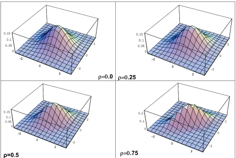
The following graphs are for standard bivariate normal distribution for different values of ρ.

-2

0

2

-2 0

2 0

0.05 0.1 0.15

-2

0

2

ρ=0.0 ρ=0.25

-2

0

2

-2 0

2 0

0.05 0.1 0.15

-2

0

2

-2

0

2

-2 0

2

0 0.05

0.1 0.15

-2

0

2

ρ=0.5 ρ=0.75

-2

0

2

-2 0

2 0

0.1 0.2

-2

0

2

Figure 3: Standard bivariate normal plots for ρ=0.0, 0.25, 0.5 and 0.75

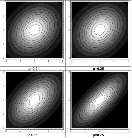
2.2 Standard bivariate normal distribution contour

The bivariate surface is perfectly understood only when the counter are drawn which are obtained by cutting bivariate normal surface with planes that are parallel to the xy-plane, and intersect at the given Z-values are heights of the parallel planes, at which these intersect the surface, as shown in Figure 4. For the Mathematica statement for contours see Appendix 3.

-2 -1 0 1 2

-2 -1 0 1 2

-2 -1 0 1 2

-2 -1 0 1 2

ρ=0.0 ρ=0.25

-2 -1 0 1 2

-2 -1 0 1 2

-2 -1 0 1 2

-2 -1 0 1 2

ρ=0.5 ρ=0.75

Figure 4: Standard bivariate normal contours plots for ρ=0.0, 0.25, 0.5 & 0.75

It is obvious from Figure 4 that, for ρ=0, the surface is symmetrical and the

contours are circular; but for ρ ≠0, the contours are ellipses which are more

3. Results

3.1 Peakedness with Mathematica

The mode in a standardized bivariate normal distribution occurs at (0, 0); and a major portion of probability is concentrated, on the volume defined by cubic:

2 1 0

4

k

k

V

=

where −k₁≤X₁≤k₁ and −k2≤X2≤ k2.

The probability that is concentrated on volume of standardized random variable

1

x and x₂ is given by

[

]

_∫∫

b

a d

c

r a X b c X d f x x dx dx

P ₁ , ₂ ( ₁, ₂) _{1 2}. (4)

To evaluate Equation (4), it can be expressed as a mixed difference equation

[

]

P_r < < < < = − − + (5)

which is a function of ρ, where F[k1,k2] is joint cumulative distribution function

(cdf).

For some selected intervals for k₁,k₂ =±1, ±2, ±3 calculated joint probabilities

are displayed in Table 1. (For Mathematica code see Appendix 3).

Table 1: Joint probabilities for ρ = 0.00, 0.25, 0.50, 0.75

2 1 X

X ρ −1< X₂ <+1 −2< X₂ <+2 −3< X₂ <+3 1

1< ₁ <+

− X 0.00

0.25 0.50 0.75 0.4661 0.4735 0.4980 0.5467 0.6517 0.6549 0.6640 0.6769 0.6808 0.6812 0.6821 0.6826 2 2< ₁ <+

− X 0.00

0.25 0.50 0.75 0.6517 0.6549 0.6640 0.6769 0.9111 0.9125 0.9171 0.9260 0.9519 0.9521 0.9527 0.9538 3 3< 1 <+

− X 0.00

0.25 0.50 0.75 0.6808 0.6812 0.6821 0.6826 0.9519 0.9521 0.9527 0.9538 0.9946 0.9946 0.9948 0.9952

It is obvious from the Table 1 that concentration of probabilities increases in each interval, with an increase in the values of ρ.

Using the same area over 4k₁k₂, another quantity, V_T, can be found, which

defines the volume that stands on the same area as given above, but whose vertical height is equal to f(0,0,ρ) as

) 1 ( 2 2 2 1 ρ π −

= k k

V_T (6)

-2 -1

0

1

2 -2 -1

0 1

2

0 0.2 0.4 0.6

-2 -1

0

1

2

Figure 5: Volume VT and standard bivariate normal together

Using Horn’s idea for measuring peakedness in the univariate distributions, we have modified it for bivariate distributions by defining

T

V V

M(ρ)=1− 0 (7)

where V₀ is the probability/volume captured in given interval by bivariate normal distribution, and V_T the total cubic volume over the given interval .

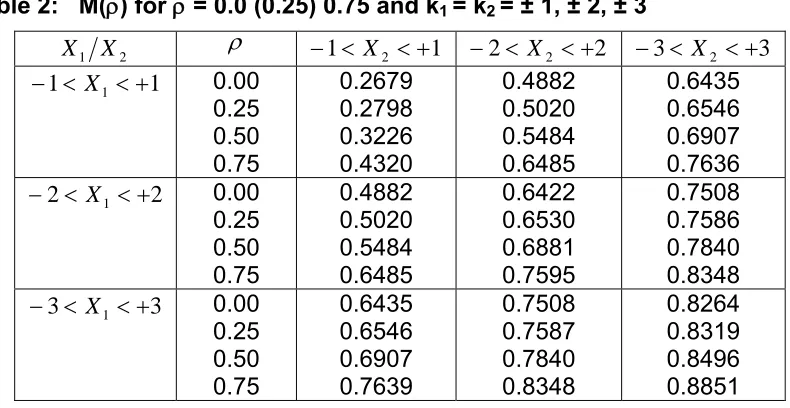
3.2 Computation for Peakedness

Some values of the parameters have been selected for the standardized bivariate normal distribution for which peakedness measure, M(ρ), has been

found, as shown in the Table 2 using Mathematica (For Mathematica code see Appendix 3).

Table 2: M(ρ) for ρ = 0.0 (0.25) 0.75 and k1 = k2 = ± 1, ± 2, ± 3

2 1 X

X ρ −1< X₂ <+1 −2< X₂ <+2 −3< X₂ <+3

1 1< 1 <+

− X 0.00

0.25 0.50 0.75

0.2679 0.2798 0.3226 0.4320

0.4882 0.5020 0.5484 0.6485

0.6435 0.6546 0.6907 0.7636

2 2< ₁ <+

− X 0.00

0.25 0.50 0.75

0.4882 0.5020 0.5484 0.6485

0.6422 0.6530 0.6881 0.7595

0.7508 0.7586 0.7840 0.8348

3 3< 1 <+

− X 0.00

0.25 0.50 0.75

0.6435 0.6546 0.6907 0.7639

0.7508 0.7587 0.7840 0.8348

It is important to note the relationship between the correlation coefficient ρ and the shape of the joint normal density. In order to get some idea as to how the shape changes with the value of ρ, let us compare the joint density in figure when ρ =0 with the given figure when ρ =0.75,0.5 and 0.25. The dependence

takes the form of a ‘squashed’ joint density. This effect can easily be seen on the equal probability contours which are circular in the case ρ = 0 and ellipses in the

case ρ ≠ 0. From the graphs in it is obvious that the more squashed the density

(and the ellipses) the higher the correlation.

4. Conclusion

Peakedness in probability distributions has been discussed extensively by using the kurtosis. There are various definitions of kurtosis in literature. However, Pearsons’s measure and Fisher’s measure are dependent on the values of the mathematical expectations or moments (i.e. μ₂,μ₄), which do not exist for some

probability distributions (for example, Cauchy) and hence it is not possible to compute kurtosis. Further, a small value of kurtosis is usually understood, as showing low peakedness and a higher value of kurtosis as showing a higher value of peakedness which in practice is not the case.

Horn’s measure has been defined even for those distributions for which moments do not exit. Also, its values are less for less peakedness and large for higher-peaked probability distributions. However, Horn’s approach just works for symmetric unimodal distributions. We propose a modification of Horn’s measure to bivariate normal distribution for evaluating peakedness. The graphs are also drawn for different values of the correlation coefficient using Mathematica. It is therefore concluded that Horn’s measure of peakedness is also useful for bivariate continuous distributions.

References

1. Abell, M. L., Braselton, J. P. and Rafter, J. A. (1998). Statistics with Mathematica. Academic Press: New York.

2. Ahmed, S. A., Haq, M. and Khurshid, A. (1990). “Measure of peakedness in Pareto model”, The Phillippine Statistician, 39, 61-70.

3. Akram, M. (1998). A comparison of the estimators of parameters in

truncated probability distributions, Unpublished M.Phil. thesis, Department of Statistics, University of Karachi.

4. Balanda, K. P. and MacGillivary, H. L. (1988). “Kurtosis: A critical review”, The American Statistician, 42, 111-119.

5. Balanda, K. P. and MacGillivary, H. L. (1990). “Kurtosis and spread”, The Canadian Journal of Statistics, 18, 17-30.

6. Blest, D. C. (2003). “A new measure of kurtosis adjusted for skewness”, Australian and New Zealand Journal of Statistics, 45, 175-179.

8. DeCarlo, L. T. (1997). “On the meaning and use of kurtosis”, Psychlogical Methods, 2, 292-307.

9. Groeneveld, R. A. and Meeden, G. L. (1984). “Measuring skewness and kurtosis”, The Statistician, 33, 391-399.

10. Haq, M., Khurshid, A. and Ahmed, S. A. (1991). “Peakedness in distributions with no moments”, Journal of Indian Society of Statistics and Operations Research, 12, 5-14.

11. Hogg, R. V. (1974). “Adaptive robust procedures: A partial review and some suggestions for future applications and theory”, Journal of the American Statistical Association, 69, 909-927.

12. Horn, P. S. (1983). “A measure for peakedness”, The American Statistician, 37, 55-56.

13. Hopkins, K. D. and Weeks, D. L. (1990). “Tests for normality and measures of skewness and kurtosis: Their place in research reporting”, Educational and Psychological Measurement, 50, 717-729.

14. Hussain, E., Haq, M. and Khurshid, A. (2000). “Peakedness in Bivaraite Normal Distribution”, Karachi University Journal of Science, 28(2), 1-8. 15. Kaplansky, I. (1945). “A common error concerning kurtosis”, Journal of the

American Statistical Association, 40, 259.

16. Kinney, J. J. (2002). Statistics for science and engineering. Addison Wesley: Reading, MA.

17. Kotz, S., Balakrishnan, N. and Johnson, N. L. (2000). Continuous multivariate distributions, Vol. 1: Models and Applications, Second edition. John Wiley: New York.

18. Mosteller, F. and Tukey, J. W. (1977). Data analysis and regression. Addison Wesley: Reading, MA.

19. Oja, H. (1981). “On location, scale, skewness and kurtosis of univariate distributions”, Scandanivan Journal of Statistics, 8, 154-168.

20. Quraishi, S. M. and Haq, M. (1999). “Peakedness in bivariate discrete probability distributions”, Karachi University Journal of Science, 27, 39-44. 21. Rose, C. and Smith, M. D. (1996). “The multivariate normal distribution”,

Mathematica Journal, 6, 32-37.

22. Rose, C. and Smith, M. D. (2002). Mathematical statistics with Mathematica. Springer Verlag: New York.

23. Ruppert, D. (1987). “What is kurtosis?” The American Statistician, 41, 1-5. 24. Sahai, H. and Khurshid, A. (2002). Pocket dictionary of statistics.

McGraw-Hill: New York.

25. Schmid, F. and Trede, M. (2003). “Simple Tests for peakedness, fat tails and leptokurtosis based on quantiles”, Computational Statistics and Data Analysis, 43, 1-12.

27. Wolfram, S. (1991). Mathematica: A system for doing mathematics by computer. Addison-Wesley: Reading, MA.

28. Wu, D. W. (2002). “Some study of kurtosis: A new measure of peakedness for distribution”, Advances and Application in Statistics, 2, 131-137.

Appendix 1: About Mathematica

Computers have been used in variety of ways to enhance the concepts in probability and statistics. A computer algebra system (CAS) such as Mathematica opens up new opportunities for developing insights. CAS creates a new paradigm for designing, analyzing and drawing conclusions from models in science and engineering. The technology in the CAS allows concepts to be paramount while computation and details become less important. A CAS can provide a deeper understanding of basic concepts and are potentially useful tools for the mathematical statistics.

With advancing technology, most work in applied statistics involves computers, but it is less common to use computers to do symbolic manipulation in mathematical statistics. However in recent years, number of books have appeared that try to hybrid statistical probability and statistical concepts using CAS Mathematica (for example, Abell et al.; 1998; Kinney, 2002; Rose and Smith, 2002).

Mathematica is general system for doing mathematical computation. It can be used in various ways for example as a (i) calculator, (ii) numerical operations, (iii) symbolic and algebraic operations and (iv) graphics. Builtin packages are available to facilitate the users. Further Mathematica has its own language, one can write own program. One of the most important things about Mathematica is that it is highly extensible. For detail see web site www.woolfram.com.

Explanation of some basic Mathematica commands used which are used in this paper:

Plot

Ÿ Plot[f, ax, xmin, xmaxa] generates a plot of f as a function of x from xmin to xmax.

Ÿ Plot[aa, a, … a, ax, xmin, xmaxa] plots several functions a.

Plot3D

Ÿ Plot3D[f, ax, xmin, xmaxa, ay, ymin, ymaxa] generates a three-dimensional

Ÿ Plot3D[af, sa, ax, xmin, xmaxa, ay, ymin, ymaxa] generates a

three-dimensional plot in which the height of the surface is specified by f, and the

shading is specified by s.

P

ContourPlot

Ÿ ContourPlot[f, ax, xmin, xmaxa, ay, ymin, ymaxa] generates a contour plot of f

as a function of x and y.

Appendix 2

(* load tke packeg once *)

<< Statistics`MultinormalDistribution` (* Run this block for differnt values of c1 *)

(* This block plots bivariate normal pdf p and its and contour *)

c1 = 0.75;

(r = {{1, c1}, {c1, 1}};

ndist = MultinormalDistribution[{0, 0}, r]); p[r_] := PDF[ndist, {x1, x2}];

p = Plot3D[p[t], {x1, -3, 3}, {x2, -3, 3}, PlotRange -> All];

c = ContourPlot[p[t], {x1, -2, 2}, {x2, -2, 2}]

Appendix 3

[(* once load the pakage *)

<< Statistics`MultinormalDistribution`]

[(*This block computes joint probability p and Horn measure pk *) (* In this block c1 is the value of correlation coefficient ndist is joint pdf *)

(* change the values of c1 for new computation *) c1 = 0.0

(r = {{1, c1}, {c1, 1}};

ndist = MultinormalDistribution[{0, 0}, r]); l[{k1_, k2_}] := CDF[ndist, {k1, k2}];

Clear[v, p, p1, pk] c1 = .75

For[i = 1, i < 4, k1 = i;

k2 = j;

vt = (2*k1*k2)/(Pi*Sqrt[1 - c1^2]); v = N[vt]

p = l[{k1, k2}] - l[{-k1, k2}] - l[{k1, -k2}] + l[{-k1, -k2}] ; p1[i, j] = p;