Decreasing and Bathtub shaped failure rate model
Mahmudul Alam
Disaster Prevention Research Institute, RECP Kyoto University, Gokasho
Uji-shi, Kyoto 611-0011 JAPAN
[email protected] [email protected]
Abstract
The maximum likelihood equations of IDB distribution can’t be solved analytically. Solutions of the MLE equations can be obtained numerically. But the problem is to detect the initial value of the parameters to solve the nonlinear MLE equations. A technique is developed for formulating the initial value of the parameter to solve the MLE equations of IDB distribution. Considering all the facts, though IDB distribution is not suitable for graduating mortality data but the model can graduate mortality data of Bangladesh in the age range of 0-8 very well.
Key words: IDB distribution, Mortality, MLE, Estimation.
Introduction
In general, mortality data shows very high frequency at and near zero age group with a sharp decline within a few years of life, then becoming more or less constant for a couple of years and again rises steadily resulting to a more or less bathtub shaped curve. The exponential power life testing, and increasing, decreasing and bathtub shaped failure rate (IDB) distribution both belonging to the mixed failure rate group have the property to produce bathtub shaped hazards as well as frequency distribution under certain conditions. The primary aim of the study is to fit mortality data from different sources including Bangladesh to IDB model and to verify the degree of fitness.
There are a number of studies dealing with models for bathtub-shaped failure rate. For example, Gaver and Acar (1979) proposed a model that has a broad range of flexibility-constant hazard to bathtub hazard under different conditions, a flexible bathtub hazard model for non-repairable systems with uncensored data (Jaisinghet al., 1987), a lifetime distribution with an upside-down bathtub-shaped hazard function (Dimitrakopoulou et al., 2007) and so on. Mudholkar and Srivastava (1993) introduced an exponentiated Weibull distribution. Xie and Lai (1996) gave another additive model with bathtub-shaped failure rate. The parameters of this model can be estimated using graphical method. An additive Burr XII model of four parameters is studied in Wang (2000). There are also several other studies that investigated the combination of two Weibull distributions for bathtub shape failure rate function, such as the competing risk model, multiplicate model, and sectional model given in Chen (2000). Graphical methods and representations of the mixed Weibull distributions were discussed in Jiang and Murthy (1995, 1999), Jiang and Kececioglu (1992) and recently Lai, et.al (2001).
Increasing, Decreasing, Constant and Bathtub-shaped failure rate distribution (IDB)
In a study of how estimation errors and model assumptions affect the costs in the optimal preventive maintenance problem, it soon became evident that for this purpose the established distributions were not always feasible. Distributions with one or two parameters like Weibull distribution impose very strong restrictions on the data. This is well illustrated by their inability to produce bathtub curves. On the other hand, more flexible distributions usually have five or more parameters (Jaisingh et al., 1987), which seem to make the study of estimation and optimization from small samples a rather hopeless numerical task (Hjorth, 1980).
A second idea leading towards the distribution was the lack of physical motivation for various bathtub models. While the Weibull distribution, the extreme value distribution, the normal distribution, and the whole class of IFR (increasing failure rate) distributions have some sort of physical motivations, the burn in argument of bathtub does not seem to have much relevance in many situations where such distributions arise. The reason for this seems to be that a probabilistic selection argument, and not a physical one, is the most relevant explanation of the bathtub curve. For practical interest with lifetime data subject to increasing age, an increasing failure rate of each individual was the natural starting point. These arguments, together with considerations of mathematical simplicity, led us to search for a new distribution, and with capacity to also describe bathtub curves. The distribution to be studied is defined by the survival function
2 2
) 1 ( ) (
t
e t
S t
The hazard function can be written as t t t t t h 1 ) ( (2)
where, = 1/and =/and,,> 0
Special cases of the IDB distribution (relation to other distribution):
= 0; the Rayleigh distribution
= = 0; the Exponential distribution
= 0; decreasing failure rate
; increasing failure rate
0<< ; bathtub curve
Methodology and materials
Primary aim of this research is to estimate the parameters of the desire distribution. The genesis and the method of estimation involved in the research is the subject matter of methodology, while a discussion about the data and the computing aids constitutes the materials. The product limit estimate (Kaplan and Meier, 1958) of the survival function S(t) is used to estimate the survival probabilities for grouped data. For models in which some transformation of the survivor function is linear in the parameters, least squares estimation can be used to estimate the parameters. But the survival function of IDB distribution
2 2 1 ) ( t e t t S (3)
which is non linear and least squares method may not be used to estimate the parameters. Since there exists no censoring expect the last interval, so the likelihood function can be written as (Lawless, 1982);
djk
j
j j S t
t S t L
1 11) ( )
( )
( (4)
Putting the value of S(t) and taking log on both sides, we have
Log
1 1 2 2 2 2 1 1 1 1 log ) ( k j t t t t j j j j j e e d t L (5)
Differentiating eq.(5) with respect to , and and setting to zero we get three non linear equations which are very difficult to solve analytically. The MLE equations are as follows
0 1 1 1 1 1 log 1 1 log 1 2 2 2 2 1 1 2 2 1 2 2 1 1
k j e t e t t e t t e t d j t j j t j j j t j j j t j j g (7) 0 1 1 1 1 1 1 2 2 2 2 1 1 2 2 2 2 1 2 2 1 1
k j e t e t t e t t e t d j t j j t j j j t j j j t j j h (8)The survival or the cumulative hazard function of IDB distribution can’t be expressed in a linear form and therefore, obtaining initial value of the parameters to solve the maximum likelihood equations (6-8) is difficult. A simple model is deduced from Kaplam-Meier non parametric method (Lawless, 1982) to search the initial value of the parameters of IDB distribution as
0 1 1 1 2 2 2 1 2 3 3 1 2 3 2 2 1 2 2 1 2 1 2 3 3 1 ) 1 ( 1 3
2
t t t c c t c t t c t t c c t t t
(9)Where ci = S(ti), i = 1, 2, 3. S(t) is computed according to Kaplan-Meier method.
Using the positive root of, the later equations can be solved.
Solution of the equations (9-11) for,andare known as the initial value of the parameter of the MLE equations. Mortality data of Japan, Canada and Bangladesh have used for fitting the IDB model. In every case, data is taken from secondary sources (Statistical Year Book and Demographic Year book). It is to be noted that these data sets are not directly observed age-specific death figures rather, these are synthesized from abridged life tables (Table 1-2).
Table 1: Observed and expected mortality indices of Bangladesh Age Group Observed Death Expected Death
0 117 177
1 20 17
2 13 11
3 10 8
4 6 7
5-9 12 34
10-14 6 37
15-19 8 43
20-24 11 49
25-29 12 54
30-34 12 56
35-39 14 58
40-44 21 57
45-49 24 55
50-54 41 52
55-59 63 47
60-64 78 42
65-69 123 37
70-74 114 32
Table 2: Observed and expected mortality indices of Canada and Japan
Age Group
Canada Japan
Observed Death
Expected Death
Observed Death
Expected Death
1 1410 1925 9969 11503
1-4 292 524 3637 4442
5-9 187 1336 2326 12000
10-14 200 2127 1717 19256
15-19 455 2856 4102 25949
20-24 476 3494 4627 31829
25-29 585 4022 5262 36727
30-34 633 4426 8863 40531
35-39 832 4701 10236 43187
40-44 1091 4848 15438 44695
45-49 1488 4874 25069 45106
50-54 2492 4789 34761 44511
55-59 3851 4609 40866 43037
60-64 5052 4350 46916 40833
65-69 7022 4033 68729 38062
70-74 8838 3675 97355 34887
75-79 10347 3293 114097 31467
80-84 11389 2905 113553 27946
85+ 19719 13572 104360 135915
Result and discussion
The value of can be found by solving eq.(6) using the initial values of β and δ. After fixing the value of (new value) and δ (initial value), the value of β can be found by solving eq.(7). Lastly, fixing the values of β (new value) and (new value) then the value of δ can be obtained by solving eq.(8). Continue the process until the convergence (less than 10-07) is obtained. Sometimes if the equation for is chosen first, after certain number of iterations, the value of t/λ may becomes <-1 and then the MLE equations can’t be solved. To avoid this situation better to choose either β or δ first and then solve for . Final estimation of the parameters is shown in table 3.
Table 3: MLE estimation of the parameters and its significance
Source Parameter Chi-square
λ β δ
Bangladesh 0.0014183789 0.029576646 0.00062557 936
Japan 6.975279E-13 0.00057389 0.00045322 796920
Canada 3.753157E-13 0.000884407 0.0004701 75713
This process is easy to find out the initial value of the parameters for MLE if we don’t have any idea about the approximate value of the parameters. As for example, if we choose the initial value for λ= 100, β= 3.0 and δ= 1.5 to solve equations (6-8), it takes a lot of time to reach the real value than that of the initial value chosen under equations (10-12) as λ= 40.017, β= 0.7178 and δ= 0.0005 for Bangladeshi data. Comparing these two initial value data sets, the iteration time for second set takes less time at least 30% than first set to solve the maximum likelihood equations until the final approximated value reach to λ= 0.0014183, β= 0.02957665 and δ = 0.0006255701. Five sets of mortality data from Japan, Canada and Bangladesh are used to verify the acceptability of the proposed technique and found almost same results (results of only three data sets are shown in this study). This technique is also applied in Jaisingh’s (1987) data set and found similar results.
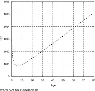
Two sets of data is used in the study of Dimitrakopoulou et al., (2007). Depending on the nature of the data sets, they have shown that the estimated hazard function may not always produce bathtub shape curve. Second data set of their study follows bathtub shaped hazard pattern like this work for Bangladeshi mortality data (Fig. 3) and first set produces unimodal pattern like Japanese and Canadian mortality data (Fig. 4).
Conclusion
To reach the initial solution of MLE equations for IDB distribution, our proposed technique may take less time to solve the MLE equations. The model used here for graduating mortality data is not found suitable, although the model fit the data of Bangladesh in the age range of 0-8 well. Development of a new model with the combination of increasing failure rate models and this model, may graduate the mortality data of Bangladesh to a better extent.
We are unable to make any comments regarding the efficiency of the estimation process in estimating parameters of the models studied. Because, the information used for estimating parameters are not from the respective distributions. A study of the efficiency of the estimation models as well as the initial solution may be taken as a problem for the future studies.
Reference
1. C.D. Lai, M. Xie and D.N.P. Murthy, Bathtub-shaped failure rate life distributions. In: Handbook of statisticsAdvances in reliability, 20, 69–104, Elsevier, London, 2001.
2. D.P. Gaver and M. Acar, Analytical hazard representations for use in reliability, mortality and simulation studies. Com.in statist., B(Sim.& Com.), 8, 91-111, 1979.
3. E.L. Kaplan and P. Meier, Nonparametric Estimation from Incomplete Observations. Journal of the American Statistical Association, 53 (282), 457-481, 1958.
4. F.K. Wang, A new model with bathtub-shaped failure rate using an additive Burr XII distribution. Reliab Engng Syst Safety, 70, 305–312, 2000.
5. G.S. Mudholkar and D.K. Srivastava, Exponentiated Weibull family for analyzing bathtub failure-rate data. IEEE Trans Reliab, 42, 299–302, 1993.
6. J.F. Lawless, Statistical models and methods for lifetime data. John Wiley & Sons, New York, 1982.
7. L.F. Zhang, M. Xie, and L.C. Tang, Bias correction for the least squares estimator of Weibull shape parameter with complete and censored data.
8. L.R. Jaisingh, W.J. Kolarik and D.K. Dey, A flexible bathtub hazard model for non-repairable systems with uncensored data. Microelectron. Reliab, 27(1), 87-103, 1987.
9. M. Xie and C.D. Lai, Reliability analysis using an additive Weibull model with bathtub-shaped failure rate function. Reliab Engng Syst Safety, 52, 87–93, 1996.
10. M.M. Alam, A study of some mixed failure rate models in graduating mortality data. Unpublished M.Sc thesis, 1996.
11. R. Jiang and D.N.P. Murthy, Exponentiated Weibull family: a graphical approach.IEEE Trans Reliab 47, 68–72, 1999.
12. R. Jiang and D.N.P. Murthy, Modeling failure-data by mixture of 2 Weibull distributions: a graphical approach. IEEE Trans Reliab, 44, 477–488, 1995.
13. S. Jiang and D. Kececioglu, Graphical representation of two mixed Weibull distributions.IEEE Trans Reliab41, 241–247, 1992.
14. S. Rajarshi and M.B. Rajarshi, Bathtub distributions—a review. Commun Stat—Theory Meth,17, 2597–2621, 1988.
15. T. Dimitrakopoulou, K. Adamidis, and S. Loukas, A lifetime distribution with an upside-down bathtub-shaped hazard function. IEEE Transactions on Reliability, 56(2), 308-311, 2007.
16. T. Zhang and M. Xie, Failure data analysis with extended Weibull distribution. Communications in Statistics—Simulation and Computation,
36, 579–592, 2007.
17. U. Hjorth, A reliability distribution with increasing, decreasing, constant and bathtub-shaped failure rates. Technometrics22, 99–107, 1980.
18. Z. Chen, A new two-parameter lifetime distribution with bathtub shape or increasing failure rate function. Stat Probab Lett, 49, 155–161, (2000). 19. Z.J. Gong, Estimation of mixed Weibull distribution parameters using the
0 50 100 150 200 250 300
0 10 20 30 40 50 60 70 80
Observe Death Expected Death
Age
Figure 1: Representation of observe and expected death for Bangladesh
0 2 104 4 104 6 104 8 104 1 105 1.2 105 1.4 105
DeathCan ExpDethCan ExpDethJpn DeathJpn
0 20 40 60 80
Age (year)
0 0.01 0.02 0.03 0.04 0.05 0.06
0 10 20 30 40 50 60 70 80
Age Figure 3: Hazard plot for Bangladesh.
0 0.01 0.02 0.03 0.04 0.05
0 20 40 60 80
HCan HJap
Age (year)