R E S E A R C H
Open Access
A selection criterion for patterns in
reaction
–
diffusion systems
Tatiana T Marquez-Lago
1,2*and Pablo Padilla
3* Correspondence: [email protected] 1Department of Mathematics and
Center for the Spatiotemporal Modeling of Cell Signaling (STMC), University of New Mexico, Albuquerque, NM 87131, USA 2
Integrative Systems Biology Unit, Okinawa Institute of Science and Technology, 1919-1 Tancha, Onna-son, Kunigami, Okinawa 904-0412, Japan Full list of author information is available at the end of the article
Abstract
Background:Alan Turing’s work in Morphogenesis has received wide attention during the past 60 years. The central idea behind his theory is that two chemically interacting diffusible substances are able to generate stable spatial patterns, provided certain conditions are met. Ever since, extensive work on several kinds of pattern-generating reaction diffusion systems has been done. Nevertheless, prediction of specific patterns is far from being straightforward, and a great deal of interest in deciphering how to generate specific patterns under controlled conditions prevails.
Results:Techniques allowing one to predict what kind of spatial structure will emerge from reaction–diffusion systems remain unknown. In response to this need, we consider a generalized reaction diffusion system on a planar domain and provide an analytic criterion to determine whether spots or stripes will be formed. Our criterion is motivated by the existence of an associated energy function that allows bringing in the intuition provided by phase transitions phenomena.
Conclusions:Our criterion is proved rigorously in some situations, generalizing well-known results for the scalar equation where the pattern selection process can be understood in terms of a potential. In more complex settings it is investigated numerically. Our work constitutes a first step towards rigorous pattern prediction in arbitrary geometries/conditions. Advances in this direction are highly applicable to the efficient design of Biotechnology and Developmental Biology experiments, as well as in simplifying the analysis of morphogenetic models.
Background
Turing models and general reaction–diffusion systems have been used to study mechanisms leading to emergent spatial patterns. Such studies have proved useful in a wide range of fields, including Biology, Chemistry, Physics, Ecology and Economics (see [1] and references therein).
Patterns arising in reaction–diffusion processes can be observed in well-known oscillatory models such as the Brusselator [2,3] and the Oregonator model [4] of the Belusov-Zhabotinsky chemical reaction. One can also observe distinct geometric patterns through the Schnakenberg and Brandeisator models, of the CIMA reaction [1], among many others. In Biology, reaction–diffusion models have been proposed to describe developmental processes such as skin pigmentation patterning [5,6], hair follicle patterning [7], and skeletal development in limbs [8]. Remarkably, even synthetic multicellular systems have been programmed de novo to generate simplified patterns using quorum sensing mechanisms [9,10], envisioning future applications in tissue
engineering [11]. In fact, it is the ability of Turing patterns to regenerate autonomously that gives them great utility in applications such as tissue engineering and developmental processes [11,12]. More recently, tomography studies of microemulsions have even revealed three-dimensional Turing patterns [13].
Due to the large applicability of pattern generating mechanisms in several research fields, understanding the relationship between reaction–diffusion parameters and specific patterns becomes essential. Up till now, heuristic criteria had been solely proposed, with restrictions on reactive terms (e.g. [14,15]). So, the main purpose of our paper is to propose an analytic selection criterion aimed at predicting patterns for general reaction– diffusion systems, depending on the nonlinearities involved in the reaction terms. We will illustrate these ideas with two different types of pattern-generating reaction–diffusion systems, namely, the Gierer-Meinhardt activator-inhibitor model (a short-range positive feedback coupled to a long-range negative feedback) [16] and the Fitzhugh-Nagumo equations [17].
For such, we will consider the general RD system
∂u
∂t ¼ D1∇
2uþf uð ;vÞ
∂v
∂t¼ D2∇
2vþg uð ;vÞ
ð1Þ
in a two dimensional spatial domainΩ, supplemented with zero flux boundary conditions. This model has been extensively used in many contexts and is by now standard (see for instance [18]). It is worth noting that, when considering a Gierer-Meinhardt system, the observed patterns are generally either spots or stripes. Correspondingly, one can observe either spots or labyrinthic-like patterns in Fitzhugh-Nagumo systems. In [19], a systematic analysis for a generic cubic nonlinearity is carried out for the first type of systems, and it is shown that the formation of spots and stripes depends on the presence or absence of a quadratic term respectively (see also [20] for more recent works on the subject). For the simplest case, namely a scalar equation in a one dimensional domain, a full analytical solution can be given in terms of the qualitative structure of the nonlinearity. Although there are no spots or stripes in this case, a simple interpretation can be given. Looking for steady state solutions leads to a classical problem in mechanics and an energy function is well defined.
With this terminology in mind, let us go back to the definition of an energy function and its use as a selection criterion. Roughly speaking, the criterion for the scalar case states that if the associated energy of the system is bistable (i.e. it has two minima) but has a unique global minimum, then spots will be formed, corresponding to the existence of homoclinic solutions. Here, it is worth keeping in mind the analogy with the mechanical case. Indeed, by solving the equation for special nonlinearities explicitly, it becomes clear that a homoclinic solution represents a spot, and that a heteroclinic solution (a front) represents a stripe. This has a simple interpretation in the language of phase transitions. Consider a two-phase system with an energy function having two minima (corresponding precisely to the stable phases), a so-called double well potential. If the minima are not at the same height, it means that one of the phases, say A, has less energy than B. If the two phases coexist, it will be energetically speaking more efficient to have a‘background’of A surrounding patches of B. If one considers a usual term in the energy that penalizes the region of transition between phases, it is natural, as it actually occurs, that the patches will be circular (i.e. spots). On the other hand, if the roles of A and B are inverted, then the situation is completely analogous, but in this case spots of phase A would appear, surrounded by a background of B. However, in the case when the minima heights are identical, there is no preferred phase in terms of the energy and the formation of more complicated structures, for instance, stripes. The scalar case is atypical in the sense that the results by Casten and Holland mentioned above establish that no spatially nonhomo-geneous patterns can be formed. In this respect, the formation of spots or stripes can only be understood in the metastable sense since, if a stable pattern is eventually achieved, it will be constant (see the numerical simulations presented in the Results section).
Our proposed criterion is a natural generalization of this fact. Using phase plane analysis and standard methods in differential equations and mechanics, we show that an analog of the energy of the system provides a clear way of predicting the pattern that will be formed. In two spatial dimensions and for general reaction diffusion systems, an extension of this criterion can be obtained by reinterpreting the results in one dimension in a probabilistic way, proposing a function that plays the role of energy. If the system itself has variational structure, then the same reasoning can be made, since a natural energy function exists. The important fact is that, even in the case where there is no variational structure (and therefore, no a priori energy function given), it can be constructed. It will be given as the solution of a Fokker-Planck equation associated with the original reaction–diffusion system.
In dynamical terms and for the scalar case, spots will be formed if the energy has a unique global minimum, corresponding to the existence of a homoclinic solution (a typical spot). Indeed, by solving the equation explicitly for special nonlinearities it becomes clear that a homoclinic solution represents a spot, and that a heteroclinic solution (a transition layer) represents a stripe. When these special cases are considered on the plane, they correspond to radial solutions for the energy with a single global minimum, and to transition layers for the double-well energy, with the bottoms of the two wells having the same height.
perimeter of a domain of a given area. For a precise mathematical formulation of these statements we refer the reader to [23].
In order to construct the analogue of the energy in the general case, we write down an associated Fokker-Planck equation for the transition probability, ρ, of the associated dynamical system, interpreting diffusion terms in the standard probabilistic way. Then we propose that -ρplays the role of the energy function, and the fact that spots or stripes are formed depends on whether it has one or more than one global minima. We then examine these criteria by means of numerical simulations. From the analytic point of view we show that, under suitable assumptions, -ρ is a Lyapunov function for the reaction–diffusion system, in the same way the energy is a Lyapunov function for the one dimensional case or, in general, when the system has variational structure. This provides a proof to the intuitive discussion on phase transitions above. Such proof is based on a well-known fact about invariant regions for reaction-diffussion systems (see below and [24] for more details). It is worth mentioning reaction–diffusion systems do not in general possess a Lyapunov func-tion, as evidenced by the fact that they may show periodic or chaotic time dependence. So, in what follows, it is important to note global Lyapunov functions are not implied.
Furthermore, we point out that our proposal generalizes the work presented in [19], in which reaction–diffusion models containing quadratic and cubic reaction terms were studied. In fact, reinterpreting these results with our criterion is straightforward, since the absence of an even term in the equation implies the absence of an odd term in the corresponding potential and therefore, the existence of two global minima, yielding stripes formation. Nonetheless, as soon as an odd term is present, there is only one global minimum, yielding spots. It is also important to mention here that these facts suggest a general result that is observed in our simulations. In these simulations, since the presence of a cubic term is generic, spot formation is expected to be the robust option. This is also true for our criterion, since the generic situation is that -ρ has only one global minimum.
Lastly, for the Fitzhugh-Nagumo system we carry out analogous simulations. The structures that are formed are spots or labyrinth-like structures and our numerical simulations suggest that our criterion is still valid, showing versatility across different types of pattern generating systems.
Methods
The Fokker-Planck associated equation
For a general two equation reaction–diffusion / Turing system
∂u
∂t ¼ D1∇
2uþf uð ;vÞ
∂v
∂t¼ D2∇
2vþg uð ;vÞ
an associated potential can be defined by minus the transition probability associated with the system
du
dt ¼ f uð ;vÞ dv
when subjected to a random perturbation determined by the diffusion coefficients. That is, by considering the system of stochastic differential equations
du¼fðu;vÞdtþ ffiffiffiffiffiffiffiffi2D1
p
dW1
dv¼g uð ;vÞdtþ ffiffiffiffiffiffiffiffi2D2
p
dW2
where the Wiener termsW1,W2are the components describing two-dimensional standard Brownian motion.
Then, the transition probability density ρ (u, v, t), i.e. the probability of finding the system in the state (u, v) at timet, satisfies the Fokker-Planck equation
∂ρ
∂tþ
∂
∂u½f uð ;vÞρðt;u;vÞ þ
∂
∂v½g uð ;vÞρðt;u;vÞ ¼
1 2
∂22D 1ρðu;vÞ
∂u2 þ
∂22D 2ρðu;vÞ
∂v2
with zero flux boundary conditions, and where
∫
∞−∞∫
∞−∞ρðu;vÞdu dv¼1 (cf. Reference [25] for details on the relationship of (1), the stochastic differential equation system, and the Fokker-Planck equation). It is worth noting the Fokker-Planck equation above is a special case of the Feynman-Kac formula, for which a solution can be analytically found. In what follows, we will obtain the stationary state solution of this equation.Calculus of variations
The calculus of variations is a broad subject dealing with optimization problems in infinite dimensions. Its applications range from the study of geodesics and other geometric problems to control theory in chemistry, economics, engineering, physics, etc. For a modern introduction we refer to P. Pedregal’s book ([26]). Here, for the sake of complete-ness, and for readers not familiar with this result, we present an informal derivation of the Euler-Lagrange equation for the scalar case corresponding to the energy functional
E uð Þ ¼
∫
Ωj∇uj2þ
F uð Þdx
whereEis defined for functionsu(x) onΩ, a domain in somen-dimensional Euclidian space. For simplicity Ω is assumed to be regular and bounded, and we will consider smooth functionsuwhich vanish on its boundary.
The Euler-Lagrange equation is a necessary condition for an interior minimum of E
to be attained at a certain functionv. More precisely, if Ehas an interior local minimum atv, then this function satisfies the Euler-Lagrange equation
∇2v−f vð Þ ¼0
whereF′(v) =f(v) and the equation is satisfied inΩwith Dirichlet boundary conditions, that isv= 0 on the boundary,∂Ω.
This equation is equivalent to the standard condition of the vanishing of the derivative for functions of one variable at point that constitute interior maxima or minima.
The proof follows directly from the observation that ifvis a minimum of
E uð Þ ¼
∫
Ω ∇u
j j2þ
F uð Þ dx;
then
for any fixed ϕ that vanishes on the boundary, and ε sufficiently small. In particular, this implies that as a function ofε(ϕandvbeing fixed), andε= 0,
d
dε E vð þεϕÞ ¼0:
Computing the previous derivative after a standard application of Leibnitz rule and integration by parts yields
E vð Þ ¼
∫
Ω ∇2v− F′ð Þv
ϕ dx¼0:
Since the previous equality holds for arbitraryϕ, it follows that the term in parentheses has to vanish identically, which gives the equation used in the paper.
Numerical discretization of reaction–diffusion system
Our code used for reaction–diffusion simulations was built in MatLab, using finite differences and backward Euler time stepping. Simulations were run until deviations between time steps were negligible. Namely, until the maximum difference between the current and previous time step of any point is less than 10-10. In some cases, such maximum difference criterion was stringently reduced to 10-16 (the epsilon of the machine) to guarantee reaching a numerical stationary solution. The Matlab built-in numerical solution of the Laplacian was used, and the left-hand side (LHS) of the discretization (i.e. the time derivative) was solved with a sparse incomplete Cholesky factorization with a tolerance of 10-10. For the right-hand side (RHS), i.e. the nonlinearity and coupling factor, u and v were solved using preconditioned conjugate gradients at every time step, with a tolerance error of 10-10. Also, zero-flux boundary conditions were enforced at every time step. All simulations were run with random initial conditions. Namely u(one morphogen case), or uand v (two morphogens case) were assigned uniformly distributed values between −1 and 1, at each spatial discretization point. Therefore, no pre-pattern was utilized.
Movies of simulations
All movies in the Supplementary material correspond to the parameters indicated in the text (coinciding with the indicated Figures). The time step for simulations was 0.01 time units. However, each frame of the movie corresponds to an accumulated simula-tion time of 100 units. Each movie has two frames per second, and shows the random initial conditions used in the first frame.
Results
Mechanical analog and role of the potential
section). If it were the case that species u essentially determines the dynamics of both morphogens, system (1) could be reduced to
∂u
∂t ¼ D∇
2u−f uð Þ; u¼u xð ;tÞ ð2Þ
the so-called shadow equation.
In this case, when the spatial domain is an interval and stationary patterns are looked for, the equation can be explicitly solved. In fact, the equation is equivalent to Newton’s equation for the motion of a particle under the action of a potential. This is the case, specifically, since we are looking for stationary patterns, and then ∂u/∂t= 0. Moreover, in one spatial dimension, the shadow equation would further reduce tod2u/dx2=f(u).
So the role of the potential is played by F(u) =− ∫f(u)du, and the spatial variable x
plays the role of time. This equation can be explicitly solved if we multiply it bydu/dx, as it is standard in classical mechanics. SinceF′(u) =−f(u),
d dx
1 2
du dx 2
þ F uð Þ !
¼0: ð3Þ
This implies that the quantity in parentheses is constant, i.e.
1 2
du dx 2
þ F uð Þ ¼E: ð4Þ
As a matter of fact, in the mechanical analog,Ecorresponds to the energy of the system. Solving now fordu/dxand integrating, we have the solution given implicitly as
∫
u xð Þ u að Þdu ffiffiffiffiffiffiffiffiffiffiffiffiffiffiffiffiffiffiffiffiffiffi
2ðE−F uð ÞÞ
p ¼x−a; ð5Þ
where we take the interval on the xaxis to be [a, b].
So far, it is straightforward to do these derivations. It is then useful to focus now on a case wherefhas two stable equilibria andu(x) is such thatuf(u) > 0 for large values of
u. This is the first nontrivial case to study since, for a single well, solutions would be trivial and would correspond to the (unique) minimum of a convex functional. To illus-trate this, let us consider F(u) = (1−u^ 2) ^ 2 +bu, where −f(u) =−4u(1−u^ 2) +b, and b varies. The case b= 0 corresponds to a bistable (double well) potential which goes to plus infinity with u. We can also analyze the cases where b≠0. The formation of spots or inverted spots or stripes can be deduced from the phase plane and correspond to homoclinic or heteroclinic solutions respectively (Figure 1). Alternatively, and recalling our discussion about phase separation, patterns would correspond to cases where there is a preferred phase with minimal energy.
of phase transition models and regularizations of the minimal surface problem (see for instance [23,28] and references therein). We illustrate this in Figure 1, where homoclinics correspond to spot-like solutions. The smaller homoclinic is associated with the well of least depth, and the larger one with the deeper well, respectively. However, it is worth noting that, since the lower amplitude homoclinics correspond to larger energies, they are also less stable. Also in Figure 1 (middle, inset) there are two symmetric transitions, corresponding to stripes.
In the case of two or three spatial dimensions the corresponding equation cannot be explicitly solved in general, but its solutions can still be characterized as the critical points of a functional. The latter would be the Euler-Lagrange equation of the“action”
∫
Ωj∇uj 2þ
F uð Þ dx; ð6Þ
for which a qualitative analysis similar to the one-dimensional case can be carried out, as mentioned in the preceding paragraph. For additional information on the topic, we refer the reader to the vast literature on variational methods and formation of localized structures (see [29]). For readers not familiar with the results and techniques of the calculus of variations, we refer to the Methods section (cf.Calculus of Variations).
So, if one considers system (1), the approach described above in one dimension can be extended to account for special nonlinearities corresponding to the gradient of a function, i.e. that have a variational structure. However, a full analytic treatment may not be always possible and alternative (numerical) methods should be adopted. Nevertheless, the interested reader should refer to the variational case section for complete details.
Selection criterion in a nutshell
A pattern selection criterion can in fact be obtained even when the system does not have a gradient structure. The idea is that the role of the potential will now be played by minus the transition probability associated with the system
du
dt ¼ f uð ;vÞ dv
dt¼ g uð ;vÞ
ð7Þ when subjected to a random perturbation determined by the diffusion coefficients. That is, the set of stochastic differential equations
du¼f uð ;vÞdtþ ffiffiffiffiffiffiffiffi2D1
p
dW1
dv¼g uð ;vÞdtþ ffiffiffiffiffiffiffiffi2D2
p
dW2
ð8Þ whereW1,W2are the components of two dimensional standard Brownian motion.
Then, the transition probability density ρ (u, v, t), i.e. the probability of finding the system in the state (u, v) at timet, satisfies the Fokker-Planck equation
∂ρ
∂tþ∇ ⋅ðρVÞ ¼
∂ρ
∂tþ
∂
∂u½f uð ;vÞρðt;u;vÞ þ
∂
∂v½g uð ;vÞρðt;u;vÞ
¼D1∂ 2ρ
∂u2þD2
∂2ρ
∂v2
ð9Þ
with zero flux boundary conditions (cf.Methodssection–The Fokker-Planck Associated Equation). As it was pointed out before, we claim thatρplays the role of the potential and it allows us to predict the appearance of a particular pattern in a given system.
We now illustrate that, depending on a relevant parameter in the activator-inhibitor system which might be negative, positive or zero, the stationary transition probability will have one or two global maxima. These cases correspond to the formation of spots, inverted spots or stripes. This is also concluded by numerically solving the corresponding Turing system. Similarly, we show that for a proposed Fitzhugh-Nagumo system, depend-ing on such a parameter, which might be positive or negative, the stationary transition probability has one or two maxima, corresponding to the formation of spots.
Gierer-Meinhardt case with one morphogen in two spatial dimensions We start by considering the scalar equation
∂u
∂t ¼ D∇
2uþ4u1−u2−bu2 ; u¼u xð ;y;tÞ ð10Þ
and present numerical evidence illustrating our selection criterion, followed up by its analytic proof. Previously (cf.Resultssubsection on ‘Mechanical analog and role of the potential’), a similar scalar case was treated analytically, albeit considering only one
In this case, we solved the associated Fokker-Planck equation
dρ dtþ
∂
∂u 4u 1−u 2
−bu2
ρ¼D ∂ 2ρ
∂u2 ð11Þ
and show that, depending on parameter b, the stationary transition probability yields one or two global maxima, corresponding to the formation of spots, inverted spots or stripes. These results are shown in Figure2.
Then, in order to check whether the parameters correspond to the expected patterns, we discretized our scalar equation (10) and solved it using a rectangular grid (14 × 14 units) with 104 grid points. We set a diffusion coefficient of D= 0.1 and adopted random initial conditions. For additional details on the numerical method, please refer to the Methods section (cf. Numerical discretization of reaction–diffusion system). We observed that, for parameters that determine spots and inverted spots (e.g.b=−0.02 andb= 0.02 respectively), the solution becomes constant as time progresses (i.e. a trivial spot or inverted spot). This is due to the fact that in one dimension nontrivial solutions are unstable. Sample simulations are shown in Figure 3. On the other hand, when we use the parameters that determines stripes, b= 0, the stationary solution can be a trivial spot or inverted spot, and the stationary solution is solely determined by initial conditions.
Moreover, depending on initial conditions, a transition layer can also be formed. For parameters that determine spots and inverted spots the latter is in fact a moving front, yielding at steady state the aforementioned trivial solution. Sample simulations are shown in Additional file 1: movies M1 and M3 (for general details of all presented movies, please refer‘Movies of simulations’within the Methods section). On the other hand, when using parameters that determine stripes, the transition layer constitutes a stationary solution (the time evolution only serves to align it to be normal to the boundary). A sample simulation is shown in Figure 3, as well as in Additional file 1: movie M2.
Now, in the scalar equation scenario, if we set V=∇ (−φ) and consider the whole range ofℝ, the stationary solution of the Fokker-Planck equation
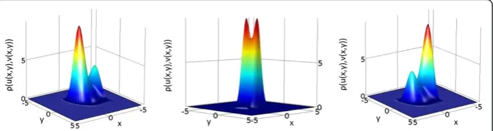
Figure 2Magnification of associated Fokker-Planck solutions of Gierer-Meinhardt model with one morphogen in two spatial dimensions.Original solutions were obtained over the domain
x∈[−3.15, 3.15]. Cases correspond to parameters (left) b =−0.02, (middle) b = 0, and (right) b = 0.02. The Fokker-Planck equation was solved in Comsol, until steady state (total time T = 1000) with a time step of 0.01, and zero-flux boundary conditions. The initial condition was defined asu xð;t¼0Þ ¼e−x2
∂ρ
∂tþ ∇ ⋅ ðρVÞ ¼ D
∂2ρ
∂u2 ð12Þ
is given explicitly by
ρð Þ ¼u exp −φð Þu
D
ð13Þ
Since–ρ andφhave the same critical points’structure, we have shown our criterion coincides with the solution obtained in the mechanical analog derived in Section 4.1. In other words, and qualitatively speaking, one can equally considerρorφin terms of the number of global minima.
Gierer-Meinhardt case with two morphogens in two spatial dimensions
We will now turn to a classical Turing system of two morphogens, u and v, in two spatial dimensions,u=u(x, y, t) andv= v (x,y,t). Namely,
∂u
∂t ¼ D∇
2uþ0:6u−r vþqu2−u3
∂v
∂t¼ ∇
2vþ1:5u−2v
ð14Þ
where we again solved the associated Fokker-Planck system of equations. We show that, depending on parameterq, the stationary transition probability yields one or two
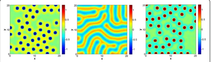
Figure 3Sample stationary solution of the Gierer-Meinhardt model with one morphogen in two spatial dimensions.Panels correspond to (left) inverted spots with b =−0.02, (center) stripes with b = 0, and (right) spots with b = 0.02. All other model/simulation parameters are indicated in the text. Simulations were run until a numerical steady state was reached (maximum difference in any lattice point less than 1e-10).
Figure 4Associated Fokker-Planck solutions of the Gierer-Meinhardt system with two morphogens in two spatial dimensions.Cases correspond to (left) q =−2 and r = 4.5, (middle) q = 0 and r = 1, (right) q = 2 and r = 4.5. The Fokker-Planck equation was solved in Comsol, until steady state (total time T = 1000) with a time step of 0.01, and zero-flux boundary conditions. The initial condition was defined asu xð;y;t¼0Þ ¼e−ðx2þy2Þ
over the domainx,y∈[−5, 5], and a diffusion coefficientD=0.04was used for morphogenu(morphogenv
global maxima (Figure 4), corresponding to the formation of spots, inverted spots or stripes. For this two morphogen case we discretized system (14) using a diffusion coeffi-cient of D= 0.04, random initial conditions, and a rectangular grid (20 × 20 units) with 104grid points (see Methods section for further details). Once again, for parameters that determine spots and inverted spots (e.g.q=−2 andq= 2 respectively) one can see that as time progresses the solution becomes constant (i.e. a trivial spot). Sample simulations are shown in Figure 5 and Additional file 1: movies M4 and M6, where it should be noted the value of parameter r was also varied, to show the desired patterns without changing the size of the simulation domain. However, if one usesq= 0, the obtained stationary pattern is stripes. The geometry of the stripes need not be straight, and stripes detach and bind to each other until all borders are normal to the boundary, soon after which a steady state is reached. Sample simulations are shown in Figure 5 and Additional file 1: movie M5.
Fitzhugh-Nagumo case with two morphogens in two spatial dimensions
Lastly, we will consider the following system with two morphogens in two spatial di-mensions,u=u(x,y,t) andv=v(x,y,t):
∂u
∂t ¼ D∇
2u−ðu−RÞu2−1−ρðv−uÞ ∂∂v
t¼∇
2v−ðv−uÞ
ð15Þ
where ϵandρare real valued constants, the diffusion coefficientDis positive and
−1 <R <1.
To show the full applicability of our method, in this last study case we will first consider the Fokker-Planck equation, from which parameter values that result in one or two maxima will be obtained. Then, we will incorporate this information into the numerical discretization of the corresponding reaction–diffusion system, corroborating the emergence of the expected patterns.
In cases such as (15), we cannot obtain a closed solution. Correspondingly, we numerically solved the Fokker-Planck equation related to system (15) (cf. Methods section, The Fokker-Planck Associated equation), iterating long enough to consider that a steady state had been reached. We obtained the results shown in Figure 6. Under these
considerations,ρdenotes the probability density distribution, whereasDis the coefficient that characterizes the disturbative strength of the statistical process.
From the numerical solution of the Fokker-Planck equation related to system (15), we obtained one set of parameters that corresponds to each pattern, namely spots or laby-rinths. However, it is important to note that these sets are not unique as many combina-tions of parameters obtained from the Fokker-Planck equation can yield the same qualitative patterns. However, the selected parameters chosen for our simulations were:
a) Spots:D= 0.04;R= 0.04;ρ= 0.3 (inverted spots with identical parameters except R= -0.04)
b) Labyrinths: identical parameters as case (a) above, exceptR= 0.
In order to test these parameters obtained through the Fokker-Planck equation, we dis-cretized the Fitzhugh-Nagumo equations in order to quickly verify if the parameters that corresponded to one or two“wells”in the Fokker-Planck steady state solution would in-deed lead to spot- or labyrinth-like patterns. In this case we used a rectangular grid ([-10, 10] × [-10, 10] units) with 104grid points (see Methods section for further details).
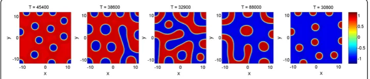
As was expected, running numerical simulations for parameters that corresponded to unequal maxima in the Fokker-Planck simulation resulted in spots or inverted spots, whereas solutions of the Fokker-Planck equation that contained equal extrema yielded labyrinthic patterns (Figure 7). Please note we did not include movies of simulations for the Fitzhugh-Nagumo system as Additional files, as stationary patterns could only
Figure 6Associated Fokker-Planck solutions of Fitzhugh-Nagumo system with two morphogens in two spatial dimensions.Cases correspond to (left) R=−0.04; (center)R= 0; (right)R= 0.04. All other simulation parameters D= 0.04,ϵ= 1,ρ= 0.3 are identical in all panels. The Fokker-Planck equation was solved in Comsol, until steady state (total time T = 1000) with a time step of 0.01, and zero-flux boundary conditions. The initial condition was defined asu xð;y;t¼0Þ ¼e−ðx2þy2Þ
over the domainx,y∈[−5, 5].
be obtained in very large time spans. By consequence, subsequent time steps portray very similar movie frames and, consequently, movie file sizes were exceedingly large. However, it should be noted distinguishable preliminary patterns are quickly formed during the first few time steps, while most simulation time is related to relaxation to stationary patterns (in many cases similar to preliminary patterns, if diffusion is slow enough).
Moreover, as can be observed in Additional file 2: Figure S1 and Additional file 3: Figure S2, the observed qualitative patterns are reproducible, and our criterion indeed predicts emergent patterns accurately. In Additional file 2: Figure S1, we present represen-tative simulations, where each row corresponds to distinct random initial conditions (used uniformly over simulations within each row), while columns correspond to variations in reaction parameterR.
Furthermore, we performed additional simulations to distinguish between effects of diffusion coefficients and reaction rates. Additional figure 3: Figure S2 shows simulations using identical random initial condition in all panels, where each row corresponds to a different diffusion coefficient, and columns again correspond to variations in reaction parameter R. As one can observe, intermediate and slow diffusion rates yield spatially inhomogeneous emergent patterns, while higher diffusion coefficient values do not.
Transient spots can slowly reduce their size and/or move through the domain until settling in their stationary position/sizes. As would be expected, systems with parameters corresponding to spot-like solutions can also yield a stationary constant solution if diffusion is fast enough. In contrast, labyrinth-like solutions do not travel throughout the domain. However, if diffusion is fast enough, a stationary constant solution will also be obtained, the value of which will depend on random initial conditions used (data not shown). These observations can in fact be theoretically expected. When the diffusion constant Dis high (e.g. system (15) with D = 0.08 or 0.16), the diffusion rates of morphogens are not different enough to generate a diffusion-driven instability. Differences between optima of the Fokker-Planck equation in each case are subsequently shown in Additional file 4: Figure S3.
Lyapunov function
It is important to notice that when the system has variational structure an analytical statement can be made (interested readers should refer to the calculus of variations section, for essentials on the topic). In such case, we can assume that there is a function φ, a potential, such that
ut¼ D1Δu− φuðu;vÞ
vt¼ D2Δv− φvðu;vÞ
ð16Þ
The system can be viewed as the Euler-Lagrange equation of the functional
∫ ∇j uj2þj j∇v2þ φðu;vÞdx ð17Þ
Moreover, this fact guarantees that any region which is invariant for the system
_
u¼−φuðu;vÞ _
is also invariant for the reaction–diffusion system in theL∞norm (see [24]). In particular, any sublevel set ofφ
IC¼ fðu;vÞjφðu;vÞ≤ Cg ð19Þ
is invariant for the differential equation (DE) system since it is by assumption a Lyapu-nov function. Notice that in the scalar case
ρ¼ eφ=ε ð20Þ
would be a solution to the corresponding Fokker-Planck equation, where ε is under-stood as above and, therefore, our criterion reduces to the one already explained. For the system case, if we assume thatφ(u,v) =φ1(u) +φ2(v), one can directly check that
eφd11þ
φ2
d2
is the solution of the associated Fokker-Planck equation, whered1andd2are given in
terms ofD1andD2above, respectively [30].
Therefore the same observation about the structure of the critical points of ρand φ that we made for the scalar case are valid here, and the criterion is rigorous in this case.
From the physical perspective, the above criterion can be justified in terms of an energy landscape for a two phase system, as discussed in the introduction. Having presented the details, it becomes clear that–ρplays the role of some effective potential for the system.
Conclusions
We have provided both analytical and numerical evidence supporting the fact that the solution of the Fokker-Planck equation associated with a reaction–diffusion system can be used in order to determine the type of emergent pattern. The following conjecture seems natural, and describes our selection criteria in a nutshell:
Assume that the stationary solution of the Fokker-Planck equation (9) has exactly two global maxima of different (equal) height. Then system (1) admits a spot-like (a stripe-like) solution.
Our presented methodology provides a powerful yet straightforward way to identify parameters yielding specific spatio-temporal emergent patterns. This is particularly important due to the prohibitive cost of computational parameter searches. Moreover, our approach is not limited by the number of equations or spatial dimensions, and general non-linearities can be taken into consideration. Hence, we believe our parameter selection criteria will greatly aid the creation of models of morphogenesis, including appli-cations in developmental biology and chemical patterns.
to use the negative of the solution of the Fokker-Planck Equation. A rigorous proof of our methodology, in this context, is current work in progress, and will be presented elsewhere.
Aside, a more detailed analytical study is needed in order to make the result applicable in more general situations. For instance, when considering heterogeneous boundary conditions, or when the domain size is not considered to be constant. Another issue worth exploring is the description of patterns as phase transitions. In other words, it seems reasonable to visualize the different patterns that emerge (from spots first, to stripes, and then to inverted spots) as parameters change as some kind of phase transition.
Additional files
Additional file 1:Movies S1-S6.Supplementary movies of Gierer-Meinhardt with one morphogen (movies M1, M2 and M3) and two morphogens (movies M4, M5 and M6).
Additional file 2: Figure S1.Sample stationary solutions of Fitzhugh-Nagumo system with two morphogens in two spatial dimensions: pattern dependence on parameter R. Cases correspond to R =–0.04,–0.02,–0.01, 0, 0.01, 0.02, 0.04, from left to right. These cases correspond to the transition from inverted spots (R =−0.04,–0.02,–0.01) to labyrinths (R = 0) to spots (R = 0.01, 0.02, 0.04). All other simulation parametersD =0.04,ϵ=1,ρ= 0.3 are identical in all panels. Different rows correspond to uniform random initial conditions used, to ensure comparability between parameter variations. Simulations were run until a numerical steady state was reached (maximum difference in any lattice point less than 1e-16, the machine epsilon). Total time until reaching steady states are shown above each case.
Additional file 3: Figure S2.Sample stationary solutions of Fitzhugh-Nagumo system with two morphogens in two spatial dimensions: pattern dependence on parameter D. Cases correspond to R =–0.04,–0.02,–0.01, 0, 0.01, 0.02, 0.04, from left to right. These cases correspond to the transition from inverted spots (R =−0.04,–0.02,–0.01) to labyrinths (R = 0) to spots (R = 0.01, 0.02, 0.04). Different rows correspond to distinct diffusion coefficients, D = 0.16, D = 0.08, D = 0.04, D = 0.02 and D = 0.01 from top to bottom. Identical random initial conditions were used in all cases, to ensure comparability between parameter variations. Simulations were run until a numerical steady state was reached (maximum difference in any lattice point less than 1e-16, the machine epsilon). Total time until reaching steady states are shown above each case.
Additional file 4: Figure S3.Absolute differences between optima of Fokker-Planck equations associated to the Fitzhugh-Nagumo system. Color-coded curves correspond to distinct diffusion coefficients of morphogenu, while points within each curve correspond to distinct values of reaction parameterRIn all cases, the Fokker-Planck equation was solved in Comsol, until steady state (total time T = 1000) with a time step of 0.01, and zero-flux boundary conditions. The initial condition was defined asu xð ;y;t¼0Þ ¼e−ðx2þy2Þ
over the domainx,y∈[–5, 5].
Competing interests
The authors declare that they have no competing interests.
Authors’contributions
Both authors participated in designing the study. TML performed analysis of the Fokker-Planck equation and all numerical solutions in this study. PP developed sections relating to mechanical analogs and variational methods. Both authors took part of the modeling, drafted, read and approved the manuscript.
Acknowledgments
TML was supported by CONACyT (Mexico, Consejo Nacional de Ciencia y Tecnologia, grant number 148724) and OIST funding. For PP, this work was partially supported by CONACyT (projects 3703P-E9607 and G25427-E).
Author details
1Department of Mathematics and Center for the Spatiotemporal Modeling of Cell Signaling (STMC), University of New
Mexico, Albuquerque, NM 87131, USA.2Integrative Systems Biology Unit, Okinawa Institute of Science and Technology, 1919-1 Tancha, Onna-son, Kunigami, Okinawa 904-0412, Japan.3IIMAS, Universidad Nacional Autónoma de México, Circuito Escolar. Cd. Universitaria, 04510MéxicoDF, Mexico.
Received: 27 November 2013 Accepted: 21 January 2014 Published: 29 January 2014
References
1. Maini PK, Painter KJ, Chau HNP:Spatial pattern formation in chemical and biological systems.J Chem Soc Faraday Trans1997,93(20):3601–3610.
2. Prigogine I, Lefever R:Symmetry breaking instabilities in dissipative systems.J Chem Phys1969,48:1695–1700. 3. Glandsdorff P, Prigogine I:Thermodynamic theory of structure, stability and fluctuations.New York: Wiley; 1971. 4. Field RJ, Noyer RM:Oscillations in chemical systems IV. Limit cycle behavior in a model of a real chemical
5. Barrio RA, Baker RE, Vaughan B Jr, Tribuzy K, de Carvalho MR, Bassanezi R, Maini PK:Modeling the skin pattern of fishes.Phys Rev E Stat Nonlin Soft Matter Phys2009,79(3 Pt 1):031908.
6. Kondo S:The reaction–diffusion system: a mechanism for autonomous pattern formation in the animal skin.
Genes Cells2002,7(6):535–541.
7. Sick S, Reinker S, Timmer J, Schlake T:WNT and DKK determine hair follicle spacing through a reaction–diffusion mechanism.Science2006,314(5804):1447–1450.
8. Miura T, Shiota K, Morriss-Kay G, Maini PK:Mixed-mode pattern in doublefoot mutant mouse limb–Turing reaction–diffusion model on a growing domain during limb development.J Theor Biol2006,240(4):562–573. 9. Basu S, Gerchman Y, Collins CH, Arnold FH, Weiss R:A synthetic multicellular system for programmed pattern
formation.Nature2005,434(7037):1130–1134.
10. Liu C, Fu X, Liu L, Ren X, Chau CK, Li S, Xiang L, Zeng H, Chen G, Tang LH,et al:Sequential establishment of stripe patterns in an expanding cell population.Science2011,334(6053):238–241.
11. Slusarczyk AL, Weiss R:Understanding signaling dynamics through synthesis.Sci Signal2012,5(220):e16. 12. Kondo S, Miura T:Reaction–diffusion model as a framework for understanding biological pattern formation.
Science2010,329(5999):1616–1620.
13. Bansagi T Jr, Vanag VK, Epstein IR:Tomography of reaction–diffusion microemulsions reveals three-dimensional Turing patterns.Science2011,331(6022):1309–1312.
14. Shoji H, Iwasa Y, Kondo S:Stripes, spots, or reversed spots in two-dimensional Turing systems.J Theor Biol
2003,224(3):339–350.
15. Uriu K, Iwasa Y:Turing pattern formation with two kinds of cells and a diffusive chemical.Bull Math Biol2007, 69(8):2515–2536.
16. Gierer A, Meinhardt H:A theory of biological pattern formation.Kybernetik1972,12(1):30–39.
17. Fitzhugh R:Impulses and physiological states in theoretical models of nerve membrane.Biophys J1961, 1(6):445–466.
18. Murray JD:Mathematical Biology. An Introduction., vol. 17.InInterdisciplinary Applied Mathematics.3rd edition. ; 2002. 19. Ermentrout B:Stripes or spots? Nonlinear effects in bifurcation of reaction–diffusion equations on the square.
Proc Roy Soc London Ser A1991,434(1891):413–417.
20. Leppanen T, Karttunen M, Barrio RA, Kaski K:Morphological transitions and bistability in Turing systems.Phys Rev E Stat Nonlin Soft Matter Phys2004,70(6 Pt 2):066202.
21. Casten RG, Holland CJ:Instability results for reaction diffusion equations with Neumann boundary conditions.
J Differential Equations1978,27:266–273.
22. Ni WM:Diffusion, cross-diffusion, and their spike-layer steady states.Notices Amer Math Soc1998,45:9–18. 23. Padilla P, Tonegawa Y:On the convergence of stable phase transitions.Comm Pure Appl Math1998,
51(6):551–579.
24. Smoller J:Shock waves and Reaction Diffusion Equations., vol. 258.New York: Springer-Verlag; 1983. 25. Pontryagin L, Andronov A, Vitt A:On the statistical treatment of dynamical systems. InNoise in nonlinear
dynamical systems.Edited by Moss F, McClintock PVE. Cambridge: University Press; 1989. 26. Pedregal P:Introduction to Optimization, Texts in Applied Mathematics Vol. 46. Springer; 2004.
27. Gidas B, Ni WM, Nirenberg L:Symmetry and related properties via the maximum principle.Comm Math Phys
1979,68(3):209–243.
28. Hutchinson JE, Tonegawa Y:Convergence of phase interfaces in the van der Waals-Cahn-Hilliard theory.Calc Var Partial Differential Equations2000,10(1):49–84.
29. Alvarez-Buylla E, Ben M, Chaos A, Cort Y, Escalera J, Espinosa C, Padilla P:Variational Problems Arising in Biology. InSingularities in PDE andthe Calculus of Variations; 2009.
30. Karatzas I, Shreve SE:Brownian Motion and Stochastic Calculus, Graduate Texts in Mathematics Vol. 113. Springer; 1991. 31. Guckenheimer J, Holmes P:Nonlinear Oscillations, Dynamical Systems, and Bifurcations of Vector Fields, Applied
Mathematical Sciences Vol. 42. Springer; 1983.
doi:10.1186/1742-4682-11-7
Cite this article as:Marquez-Lago and Padilla:A selection criterion for patterns in reaction–diffusion systems.
Theoretical Biology and Medical Modelling201411:7.
Submit your next manuscript to BioMed Central and take full advantage of:
• Convenient online submission
• Thorough peer review
• No space constraints or color figure charges
• Immediate publication on acceptance
• Inclusion in PubMed, CAS, Scopus and Google Scholar
• Research which is freely available for redistribution
![Figure 1 Solutions ofu'' (x) + 4 u(x) [1 − u(x)2] − b = 0, the stationary shadow equation in onedimension](https://thumb-us.123doks.com/thumbv2/123dok_us/308206.1523288/8.595.118.478.88.304/figure-solutions-ofu-x-stationary-shadow-equation-onedimension.webp)