R E S E A R C H
Open Access
Testing the Rasch model with the
conditional likelihood ratio test: sample size
requirements and bootstrap algorithms
Rainer W. Alexandrowicz
1*and Clemens Draxler
2*Correspondence: [email protected] 1Department of Psychology, Applied Psychology and Methods Research Unit, Universitaetsstr. 65, 9020 Klagenfurt, Austria Full list of author information is available at the end of the article
Abstract
Background: The Rasch model allows for a conditional likelihood ratio goodness of fit test. The speed of approximation of the test statistic to the limiting distribution as a function of sample size and test length has not been analyzed so far. Three bootstrap simulation methods are analyzed with respect to their performance in providing a proper distribution of the test statistic under the null- and the alternative hypothesis. Results: We found a stable approximation to the limitingχ2-distribution for sample sizes of at least 500 and 10 items. The three bootstrap algorithms rendered consistent results for theH0-cases but not for theH1-cases.
Conclusion: A sequential probability sampling scheme proves sufficiently apt for generating samples under the alternative hypothesis. This superiority can be justified from a theoretical point of view.
Keywords: Rasch model, Conditional likelihood ratio test, Bootstrap analysis, Sequential importance sampling, Number of bootstrap samples
AMS Subject Classification: Primary 62F40; 62G09; 62G10; 62H10; 62E17; secondary 91B70
1 Introduction
The dichotomous logistic model according to Rasch (1960, 1966; henceforth denoted as Rasch Model, RM) allows for assessing its adequacy for describing a given data set by means of a conditional Likelihood Ratio Test (LRT; Andersen 1973). The test statistic is
approximatelyχ2-distributed if the sample sizen→ ∞. Hence, small samples will
deteri-orate inference, i.e. the limiting distribution will not provide sufficiently precise quantiles for a reasoned decision and we have to switch to the bootstrap (cf. Efron and Tibshirani 1998), which is computationally demanding.
However, no systematic investigation has been undertaken so far to analyze the rate of approximation of the test statistic to the limiting distribution. It is therefore difficult to
decide when it is safe to use theχ2-distribution or when a bootstrap is required. This
question shall be tackled in a simulation study. Moreover, if we switch to the bootstrap, precision depends on the number of bootstrap samples. A concrete guideline will be given, how many bootstrap replications are required to fulfill a desired precision criterion.
© 2016 Alexandrowicz and Draxler.Open AccessThis article is distributed under the terms of the Creative Commons Attribution
The following outline shall guide the reader through the details of this study:
Theoretical Background We start with explaining the fundamentals of the Rasch Model (Section 2.1) and the essential basics of model parameter estimation
(Section 2.2) to an extent required to understand the simulation procedures applied in the study. Section 2.3 shows the basics of the LRT, the test statistic of which the study focusses. The task of determining the speed of approximation of the test statistic to its limitingχ2-distribution breaks down into three separate questions,
which are formulated in Section 2.4.
Methods In order to perform the simulation study, bootstrap samples in line with the RM have to be generated. For that purpose, several algorithms are at our disposal, which are introduced in Section 3.2. The study considers the distribution of the test statistic under both the null and the alternative hypothesis. These two scenarios require different simulation strategies, which are explained in Section 3.1. The simulation study covers numerous different scenarios, which may arise in practical application. Section 3.3 lists the simulation parameters considered for that purpose. Results The complex details of the study are split into results concerning theH0-case
(Section 4.1) and theH1-case (Section 4.2). Finally, Section 4.3 introduces a flexible
formula to compute an adequate number of bootstrap samples, if this procedure is required.
2 Theoretical background
2.1 The Rasch model (RM)
The RM is a discrete probability model of a Bernoulli variable,Xvi ∈ {0, 1}, assuming two
real valued parametersθv(v=1. . .n) andβi(i=1. . .k),
P(Xvi=xvi)=
exvi(θv−βi)
1+e(θv−βi). (1)
A typical application of model (1) is psychometrics, withθvdescribing respondent’sv
ability to solve a task (or item) andβi describing the difficulty of task (or item)i. Both
parameters are unbounded in value, i.e.θv,βi ∈ R. By means of the substitutionsξv =
exp(θv) andi = exp(−βi)we yield the so-called multiplicative notation of the model
equation,
P(Xvi=xvi)= (ξvi)
xvi
1+ξvi
. (2)
Due to the exponentiation, ξv and i take positive values only, and i is
inter-preted as an item easiness parameter. Conditional on both parameter vectors θ =
(θ1,θ2,. . .,θv,. . .,θn)T and β = (β1,β2,. . .,βi,. . .,βk)T the binary responses are
assumed to be independent so that the joint distribution of allnresponses to allkitems
ist given by the product of (1) (or (2), respectively) overvandi. This assumption is usually
termed conditional or local independence.
The RM is a member of the exponential family (cf. Molenaar 1995, p. 41) with the
sums Rv = iXvi and Si = vXvi being the sufficient statistics for the
parame-tersθvandβi, respectively. The separability theorem (Fisher 1922) applies (Rasch 1966,
items used (given the items are in line with the model and the model holds for all respondents).
2.2 Parameter estimation
Several parameter estimation methods have been developed. Most straightforward from maximum likelihood theory is the Unconditional Maximum Likelihood approach (UML; or Joint Maximum Likelihood, JML; cf. Baker and Kim 2004, ch. 5.6). Here we deter-mine estimates for both parameter vectors simultaneously by finding the maximum of
the unconditional likelihood function as a function ofθandβ. This is achieved by setting
the partial derivatives equal to zero and applying the pertinent numeric methods to solve a system of nonlinear equations (cf. ibid., p. 136). However, this approach suffers from the so-called incidental parameter problem as expressed in Neyman and Scott (1948). While the item parameters appear as structural (or fixed) parameters, the person param-eters constitute a random draw from the population and are therefore incidental (or nuisance) parameters. The simultaneous appearance of both kinds of parameters may cause inconsistent item parameter estimates. Corrective procedures have been proposed (cf. Molenaar 1995, p. 43), but there was dispute concerning their effect (cf. Baker and Kim 2004, ch. 5.6.2).
Generally, this incidental parameter problem may be overcome by marginalization or conditional inference (cf. Pawitan 2001, p. 274). In the first case (Marginal Maximum
Likelihood estimation, MML, cf. Baker and Kim 2004, ch. 6), the incidental parametersθv
are replaced by assuming a proper distributionG(θ)in the population (e.g. the normal),
requiring only the hyperparametersτ ofG(θ)to be determined (i.e. the mean and the
variance ofG(θ)in our example). Although this solves the incidental parameter problem,
the correct choice ofG(·)is decisive for obtaining correct estimates (cf. Molenaar 1995,
p. 47).
The second approach is the Conditional Maximum Likelihood estimation method (CML; Andersen 1970), directly involving the parameter separability feature. At its heart, this method overcomes the incidental parameter problem by conditioning on each respondent’s observed value of the nuisance parameter’s sufficient statistic, i.e. the
scorerv, when estimating the item parameters. The conditional likelihood functionLC
of the item parameter vector = (1,2,. . .,i,. . .,k)T given the vector of scores
r=(r1,r2,. . .,rv,. . .,rn)T can be written as
LC(|r)=
v
i xvi
i γrv
. (3)
The termγr denotes the elementary symmetric function of orderr, covering a
com-plex combinatorical task (cf. Andersen 1972; Formann 1986; Gustafsson 1980). Expres-sion (3) plays a crucial role in the conditional Likelihood Ratio Test (LRT; see next Section).
In the CML context, the person parameters are determined in a separate step,
where the βˆi are assumed to be the true item parameters and the θˆv are obtained
using maximum likelihood estimation (cf. Hoijtink and Boomsma 1995). Because the
the same score will obtain the same ability estimate, which will be termed θˆr or ξˆr, respectively.
In terms of the Rasch Model, items being never or always solved (i.e.si =0 andsi =n)
are infinitely difficult or easy, respectively. The same applies to respondents solving either
no item or all items (i.e.rv=0 andrv=k). While this is seldom a problem for the items
(it is unlikely that in a sample of reasonable size an item is never or always solved), it may constitute a problem for person parameter estimation, especially, when the instrument
is short (i.e.kis small). However, practicioners demand estimates for all respondents, so
we have to make further assumptions in order to obtain parameter estimates for such cases as well. These may be obtained with the Weighted Maximum Likelihood Estimation Method (WLE; Warm 1989). Based on a Bayesian argument, person parameter estimates are decreased in their absolute value, thus attenuating their unbounded growth.
2.3 Assessing model fit
Numerous methods for assessing the adequacy of the RM have been proposed, an overview of which can be found in Glas and Verhelst (1995). The present study focusses on the conditional Likelihood Ratio Test (LRT, Andersen 1973; Kreiner and Christensen 2013), which relies on the CML estimation method.
If the model holds, item parameter estimates do not differ across subsamples but for random variation (invariability assumption, cf. Engelhard Jr. 2013). The LRT allows for an assessment of this assumption by comparing the conditional likelihood of the entire
dataset according to Eq. (3), henceforth denotedL0, with the product of the conditional
likelihoods obtained from subsetsj=1. . .gof the data set,
L1=
g
j=1
L(Cj)
(j)|r(j). (4)
Andersen (1973) has shown that the quantity
Z= −2 logL0 L1
(5)
follows asymptotically a centralχ2-distribution with
df =(k−1)(g−1), (6)
given that the Rasch Model is the true model and the subsample sizes n(j) −→ ∞
(ibid., p. 128). Andersen referred to a split according to the score rv, however, one
may apply a criterion of substantive interest, like sex, treatment group, or a random split. In many applications, two groups are formed at the median of the score distri-bution. Without loss of generality, we will consider this median split in the present study.
2.4 Study purpose
The present study targets the following three questions:
Q1 How close fits the sampling distribution of (5) the centralχ2-distribution for small
to lack of approximation? This question is analyzed for both theH0-case of model fit
(Results, Section 4.1) and for model violations under a givenH1(Results, Section 4.2).
Q2 Second, do three pertinent bootstrap methods differ with respect to their preciseness in providing appropriate approximations of the type-I-error probability? These results are part of the tables of Sections 4.1 and 4.2.
Q3 And third, if a bootstrap is applied, which number of bootstrap replicates is required to obtain a sufficiently stable estimate of the desired quantile for theH0case (Results,
Section 4.3)?
3 Methods
The three questions shall be tackled by means of a simulation study, determining the
sampling distribution of the test statistic (5) for various combinations ofnandk. Usually,
a simulation study starts with fixing the population parameters of interest and drawing
samples from this population. In our case, this would comprise fixing a set ofk item
parameters andnperson parameters (ork−1 person parameters associated with each
scorer, respectively). However, the CML approach relies on the sufficient statistics of the
person parameters. We would, therefore, have to find thoserv, which are associated with
a given set of person parameters and item parameters. This task is difficult to achieve, hence we developed the following procedure:
• First, a set ofk item parametersβ∗andn person parametersθ∗is fixed, representing the population of interest. The item parametersβ∗were chosen equidistantly from the interval[−1, 1]and person parametersθ∗were randomly sampled from the
N(0, 1).
• Then, an initial sampleX0of sizen×kin line with the assumptions of the Rasch
Model is drawn from this population, yielding the realized values of the initially chosen parametersand the according sufficient statistics. The parameter estimates
ˆ
β0andθˆ0of this initial sampleX0supersede the initially chosenβ∗andθ∗. We now
dispose of both the parameter values and the accompanying sufficient statistics, which are required for the bootstrap algorithm introduced in Section 3.2.3.
The sampleX0serves as the basis for the generation of bootstrap samples providing the
distribution of the test statistic (5).
3.1 Sampling under the null and the alternative hypothesis
In order to obtain an inital data setX0providing for the distribution of the test statistic
under the null hypothesis of model fit, we take the overall parameter vector β0. This
choice assumes no subgroup characteristics to be present.
In contrast, a data set X0 providing for the distribution of the test statistic under
the alternative hypothesis is attained by separately bootstrapping j = 1. . .g
subsam-ples of size n(j) using the original subsamples’ item parameter estimates βˆi(j). These
subsample parameter vectors will necessarily differ, at least by chance, i.e. βˆ(1) =
ˆ
β(2) = . . . = ˆβ(j) = . . . = ˆβ(g). Merging these subsamples to one bootstrap
sam-ple of size n = jn(j) will therefore result in a sample violating the item invariance
item parameter differences of the βˆ(j). If we now apply the LRT in the usual man-ner, the bootstrap distribution of the test statistic represents its distribution under the alternative.
3.2 Generating bootstrap samples
Several methods for generating bootstrap samples in the context of the RM have been proposed, two of which have gained some popularity. A third method, which to the authors’ knowledge has not been described in the context of the Rasch Model before, is introduced in Section 3.2.3. These methods may cause differing distributions of the LR test statistic for reasons outlined below, what might affect the conclusions in an unpre-dictable manner (cf. Q2 in Section 2.4). Therefore, all three methods will be applied parallel in order to evaluate their impact upon the resulting distribution of the LR test statistic.
Note that the Nonparametric (or “Naïve”) Bootstrap (cf. Davison and Hinkley 1997) is not suited for generating bootstrap samples in the CML context. This has theoretical reasons, which are elucidated in the light of the present findings in Section 5.3.
3.2.1 A “Normal” Approach
In the conditional estimation approach, unbiased item parameter estimates will be attained irrespective of the actual ability distribution. Therefore, the first simulation
method uses only the item parameter estimatesβˆ0, while the person parameters are
sam-pled from a freely chosen distribution. In our case, this was theN(0,σ2), with randomly
chosen but not too extreme values ofσ2. For notational ease, the hat will be omitted in
the following.
The normal distribution has been chosen for it is arguably a proper candidate for numerous characteristics frequently assessed in those areas of social science, where
the Rasch-Model is typically applied. This approach will be termednormal marginals,
although, of course, the row marginal sumsr1. . .rnare discrete by nature; it is the under-lying parameters that are sampled from the normal. The method has been described in van den Wollenberg (1982) and has gained some popularity for generating data compliant with the RM, wherefore it is considered in the present analysis.
3.2.2 Remaining with the observed
Here we use both the person parameter estimates and the item parameter estimates
obtained fromX0. The probability of a positive response is determined by using Eq. (1)
and the according parameter estimatesθˆvandβˆi. However, this method raises two issues:
First, the CML method only allows for obtaining the item parameter estimatesβˆi. For
the estimation of the person parametersθv, the item parameter estimatesβˆi are taken
as if they were the true parameters βi. Hence, the random error associated with the
item parameter estimates remains unconsidered, possibly rendering the person param-eter estimates deficient. This could dparam-eteriorate the bootstrap procedure to an unknown extent.
Second, the ML estimate for respondents solving no item or all items would tend towards plus or minus infinity. Three ways of handling this situation could be thought of:
systematically attenuates the person parameter estimates, making the implications for our bootstrap procedure imponderable.
(ii) The WLE could be inserted only for respondents withr=0andr=k, and the ML estimates otherwise. This would probably reduce the problem largely, as in most cases only few respondents (compared to the total sample size) will realize such scores. This method is implemented in theWinMIRAsoftware of von Davier (2001), for example. (iii) One can deliberately use arbitrary values for respondents withr=0andr=k, for
example±15, so that the resulting score will almost surely be equal to 0 ork. Such a method is applied in the software packageM-Plus(Muthén 1998–2004; p. 35).
However, any of these three approaches is heuristical and thus has to be considered as unsatisfactory from a statistical point of view.
Because the intention is to maintain the original ability distribution as far as
pos-sible, method (iii) was applied in the present study. Nevertheless, this approach
will not preserve the individual scores rv. Therefore, this approach will be termed
free marginals, because the marginal scores are likely to differ from the original ones.
3.2.3 The Rasch point of view
In contrast, a sequential importance sampling procedure following a truly conditional approach will be taken into consideration. It merely regards the conditional pattern probabilities in the way they are used in the CML estimation method. Here, the
suf-ficient statistics rv for the person parameter estimates are conditioned upon, making
any distributional assumptions superfluous. The probability of a response vectorxv =
(xv1,. . .,xvk)conditional on the score equals
P(xv|rv)=γr−v1
i xvi
i . (7)
The algorithm starts with a respondent’s observed score and computes his or her probability of solving the first item
P(xv1=1|rv)=γr−v11γrv−1. (8)
Then, we transform this response probability to a manifest response by comparing it
to a random numberudrawn from the standard uniform distribution, i.e.u ∈ U(0, 1).
IfP(xv1 =1|rv)exceedsu, the bootstrap respondent’svfirst manifest responsexv1is set
to one and otherwise to zero (cf. van den Wollenberg 1982, p. 88). In case the response
evaluates to one, this person’s score rv is reduced by one, otherwise not, yielding the
modified score after step one, rv(1). The procedure continues with the second item in
the same manner and proceeds until all kitems have been processed. As soon as the
modified score afteristeps,r(vi), equals zero, the probability of solving one of the
remain-ing items has zero probability and the correspondremain-ing responses are set to zero. Ifrv(i) at
any stepiequals the number of the remaining items, all remaining responses are set to
one.
That way, each individuals original scorervis maintained, which is equivalent to fixing
fixed marginalsin the following. Nevertheless, the items’ sufficient statistics still vary according to the probability distribution described by the RM, which is the information the LRT relies upon.
3.3 Simulation parameters
The simulation comprisedk=5, 10, and 15 items andn=100, 250, 500, 750, 1000, 2500,
and 5000 observations. To each of the 21 possible combinations arising, which will be
denoted designs, the three bootstrap algorithms (normal, free, and fixed) for both theH0
and theH1case were applied. According to Eq. (6), the degrees of freedom were 4, 9, and
14, respectively.
One crucial aspect of the present study is to differentiate between inaccuracies due to a lack of approximation of the actual distribution of the test statistic to the limiting dis-tribution (i.e. a truly statistical problem) on the one hand and an inaccurate bootstrap distribution due to an insufficient number of bootstrap samples (i.e. a merely
techni-cal problem) on the other hand. Preliminary trial runs suggested that m = 200,000
bootstrap replications seem to suffice for the required distinction. Assuming that this number of bootstrap replicates makes the bootstrap caused (i.e. technical) error negligi-ble, any remaining deviation from the limiting density will be attributable to a true lack of approximation.
In order to determine the minimum number of bootstrap replicates required for a sufficiently good approximation of the bootstrap densities to the true ones under the
null hypothesis (i.e. Q3 in Section 2.4), random samples of decreasing size m∗ < m
have repeatedly been drawn with replacement from the original 200,000 samples of each
design. The following values were chosen form∗: 500, 1000, 1500, 2000, 2500, 5000, 7500,
10,000, 15,000, 20,000, 25,000, 50,000, 100,000, and 150,000. Each draw of sizem∗was
repeated 1000 times (m∗∗) in order to obtain a distribution of the LR test statistic for
eachm∗.
The densities obtained by means of the bootstrap will be depicted using kernel density estimators with bandwidth parameters of 0.2 to 0.5. The simulation itself was performed
with the programGanz Rasch(Alexandrowicz 2012), which supports all three
simula-tion techniques introduced in Secsimula-tion 3.2. The simulasimula-tion results were analyzed with R (R Core Team 2015).
4 Results
The results of the simulation study regarding questions Q1 and Q2 are presented
sepa-rately for theH0- and theH1-case (Sections 4.1 and 4.2). Section 4.3 covers the results
regarding question Q3, the required number of bootstrap samples.
4.1 Approximation under the null hypothesis
In order to describe the approximation of the bootstrap distributions to the limit-ing ones, we opposed the first four moments and selected quantiles of the estimated and the theoretical distribution of the test statistic; This step is accompanied by a
density plot of the respective distributions. Second, the p-values of the LRT
4.1.1 Descriptive approach
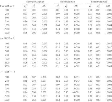
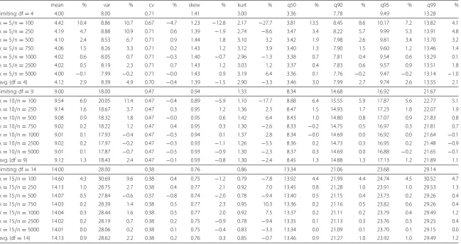
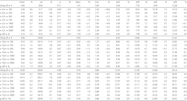
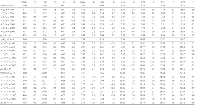
Tables 4, 5 and 6 in the Appendix show the sample statistics of the 21 different designs for the fixed, the free, and the normal marginals case. The simulated values are opposed to
the respective values of theχ2-distribution with the according degrees of freedom (first
row in each block). Each pair of columns denotes the estimated value of the statistic along with the relative deviation (in %) compared to the exact value of the limiting distribution. Two tendencies are discernible across all designs: The largest deviations can be found for
the smallest sample size (n= 100) combined with the fewest items (k = 5, i.e.df =4).
For example, in the fixed marginals case (Table 4), the mean deviates by 10.4 % for 5 items and 100 observations, by 6.0 % for 10/100, and by 4.3 % for 15/100. In comparison,
with 5000 observations, the respective deviations were−0.1 % (k = 5), 0.1 % (k = 10),
and<0.1 % (k=15).
Comparing the three simulation algorithms reveals the smallest relative deviation to appear for the bootstrap technique using normal marginals. For example, the relative error regarding the 95 %-quantile (being most important for hypothesis testing) is 2.2 %
(df = 4), 1.2 % (df = 9), and 0.9 % (df = 14). The respective figures for the fixed
marginals case are 2.6 %, 1.2 %, and 1.0 %, while the normal marginals produces deviations of 0.8 %, 0.5 %, and 0.6 %.
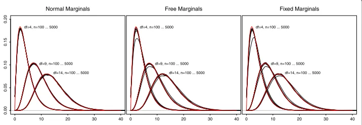
The density plots (Fig. 1) allow for a rough assessment of the overall fit of the boot-strap distributions. The plot is threefold (normal, free, and fixed marginals) with three
clusters of densities according to the df. Each line represents a certain sample size
(i.e. seven per cluster). As can be seen, the seven lines per method and df cannot be
kept apart in any of the plots, therefore no attempt was made to label the lines. Also, three lines indicating the limiting densities with the respective degrees of freedom have been superimposed (red lines). However, they mostly disappear in the three clusters, indicating overall agreement of the bootstrap generated distributions with the limiting distributions.
In the normal marginals case (Fig. 1, left hand plot), we would virtually identify no deviation of the bootstrap densities from the limiting ones. This observation was independent of the degrees of freedom and the sample size. In the other two cases (free and fixed marginals), one line per cluster seems somewhat dislocated, indicating
a reduced probability of smallerχ2-values and slightly heavier tails (the latter is hardly
df=4, n=100 ... 5000
df=9, n=100 ... 5000 df=14, n=100 ... 5000 Normal Marginals
0 10 20 30 40
0.00
0.05
0.10
0.15
0.20
df=4, n=100 ... 5000
df=9, n=100 ... 5000 df=14, n=100 ... 5000 Free Marginals
0 10 20 30 40
df=4, n=100 ... 5000
df=9, n=100 ... 5000 df=14, n=100 ... 5000 Fixed Marginals
0 10 20 30 40
discernible). These lines represent then=100 cases, in which the approximation seems deficient.
For both the free and the fixed marginals method (Fig. 1, middle and right hand plot),
the bootstap densities fordf =4 are located beyond the limiting distributions. The
den-sities coveringdf = 9 show the same tendency but to a much slighter extent, and when
df = 14, this effect vanishes entirely. The free and the fixed marginals method seem not
to differ with respect to this issue. Therefore, we can conclude that the approximation improves with the degrees of freedom, which is in line with theory. Roughly ten degrees of freedom seem sufficient for the approximation to be considered satisfactory, given a sample size of at least 250.
4.1.2 Inferential Approach
In order to compare the bootstrap distributions with the according limiting ones, we used the Kolmogorov-Smirnov (K-S) test (cf. Thode 2002, ch. 5.1.1) to test the null hypothesis
that the bootstrap distributions follow aχ2-distribution with the respective degrees of
freedom (i.e. 4 in the 5-items designs, 9 in the 10-items designs, and 14 in the 15-items designs). The results are given in Table 7 in the Appendix.
Many of the tests yield a significant result using a type-I error risk of 5 %.
How-ever, we recognize some non-significant results for (a) larger samples and (b) larger
instruments: Non-significant results were obtained for the combinations (k/n) 5/5000
(fix), 10/1000 (free+nv), 10/5000 (nv), 15/750 (nv), 15/2500 (fix+free), and all three
combinations 15/5000. The normal marginals appeared slightly better, as 4 out of 21 tests were not significant, opposed to 3 out of 21 for both the fixed and the free marginals cases. This is in line with the findings based on the descriptive statistics above.
Note that the K-S-tests rely on 200,000 bootstrap samples each, hence they are by far overpowered. Assuming that the probability of an error of the second kind almost vanishes with such large samples, a non-significant result corroborates our supposi-tion that the bootstrap distribusupposi-tion in fact realizes the limiting distribusupposi-tion. Therefore, the mere fact that at least some of the tests were not significant is in fact a
remark-able result. If we further look at the values of the K-S test statisticsD: None of them
exceeds 0.07 (which appeared with 5/100, fixed marginals algorithm). The K-S test evaluates the maximum difference of the CDFs of the bootstrap generated distribu-tions and the limiting ones, which diverge at most by 7 % in the cases considered here.
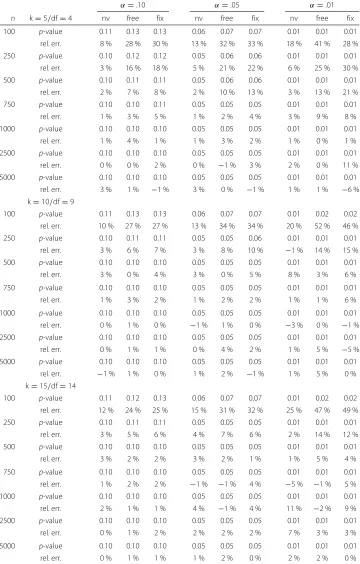
4.1.3 Comparison of the p-values
Two comparisons shall enhance conclusions from a practical point of view: First, we emulate the action a person ignorant of approximation problems might take. This
means, we simply use the seeked quantile of the limitingχ2-distribution (e.g. 9.49 for
α = 0.05 and df = 4) and decide whether or not to retain the H0. For that
pur-pose, we calculated thep-value theχ2-quantile of the limiting distribution would yield
when applied to the according bootstrap distribution (reflecting the proper probability
measure). The (relative) difference of thep-value to the nominalαquantifies how
for the three simulation algorithms, considering critical values of α = 0.10, 0.05, and 0.01.
Thep-values were considerably increased for small samples, yielding differences of up
to 52 % (α =0.01,n=100,k=10, nv). Generally, sample sizes 100 and 250 and (in some
instances) 500 would lead to substantially more significant results if we decided to use the quantiles of the limiting distribution rather than the bootstrap-based ones. Comparing the three simulation algorithms revealed that the normal marginals procedure performed somewhat better than the free and the fixed marginals algorithm. However, the discrep-ancies of the three methods are mostly moderate. Further, errors are more pronounced for low values of the type-I-error risk. As soon as samples exceed 500 observations, the deviations become increasingly smaller.
Remember that each bootstrap analysis is based on an actual realization of the test statistic (5), allowing for a second check: Table 1 compares the observed values of these
test statistics applied to both the limitingχ2-distribution and to the respective bootstrap
generated distribution. As can be seen, most differences seem negligible. This is not sur-prising, because we now consider values far away from the regions relevant to inferential decisions (i.e. the distributions’ tails). Hence too heavy tails of the bootstrap distributions
Table 1Comparison ofp-values of the observed test statistics evaluated at both the limiting and the bootstrap distribution
Normal marginals Free marginals Fixed marginals
k=5/df=4 χl2 χb2 Diff. χl2 χb2 Diff. χl2 χb2 Diff.
100 0.01 0.01 0.000 0.01 0.01 0.001 0.01 0.01 0.000
250 0.97 0.97 0.001 0.97 0.96 0.008 0.97 0.96 0.008
500 0.03 0.03 0.000 0.03 0.03 0.001 0.03 0.03 0.000
750 0.39 0.39 0.000 0.39 0.39 0.004 0.39 0.38 0.007
1000 0.69 0.69 0.001 0.69 0.68 0.004 0.69 0.68 0.004
2500 0.44 0.44 −0.001 0.44 0.44 0.000 0.44 0.44 0.001
5000 0.96 0.96 0.001 0.96 0.96 0.000 0.96 0.96 −0.001
k=10/df=9
100 0.48 0.46 0.017 0.48 0.43 0.046 0.48 0.43 0.049
250 0.32 0.32 0.006 0.32 0.31 0.010 0.32 0.31 0.010
500 0.96 0.95 0.002 0.96 0.96 0.000 0.96 0.95 0.002
750 0.63 0.63 0.002 0.63 0.63 0.004 0.63 0.63 0.000
1000 0.79 0.79 −0.002 0.79 0.79 0.000 0.79 0.79 0.001
2500 0.26 0.26 0.000 0.26 0.25 0.000 0.26 0.25 0.001
5000 0.31 0.31 0.000 0.31 0.31 0.002 0.31 0.31 0.002
k=15/df=14
100 0.08 0.07 0.006 0.08 0.07 0.011 0.08 0.07 0.010
250 0.60 0.59 0.007 0.60 0.58 0.012 0.60 0.59 0.009
500 0.07 0.07 0.001 0.07 0.07 0.002 0.07 0.07 0.003
750 0.58 0.58 0.001 0.58 0.57 0.002 0.58 0.58 0.000
1000 0.96 0.96 0.002 0.96 0.96 −0.001 0.96 0.96 0.001
2500 0.34 0.34 0.003 0.34 0.34 0.000 0.34 0.34 0.001
5000 0.63 0.63 0.001 0.63 0.63 0.000 0.63 0.63 0.000
Notes:χ2
l : limiting distribution of the test statistic;χ
2
are compensated by regions of decreased probabilities for lower values of the test statistic.
4.2 Approximation under the alternative hypothesis
The analysis of the three bootstrap methods under the alternative refers to comparing the observed differences between the three methods with the given sample sizes. At
this point, we have to keep in mind that each original sampleX0constitutes a random
realization of a population distribution of its own, hence the bootstrap generated dis-tributions of the test statistic differ across the various designs (i.e. each combination of
number of itemsk and sample sizen) and are therefore incomparable. Any attempt to
achieve the same subgroup parameter would go beyond the objectives of the present study.
Table 2 shows the descriptive statistics for the three bootstrap methods. We see
con-siderable differences in some cases: For example, in the k = 5/n = 250 design,
the mean of the bootstrap distribution generated with the normal marginals method is more than three times larger than in the free or the fixed marginals case (the
lat-ter two being fairly similar). A similar tendency occurs in the k = 5/n = 750
design, also for the normal marginals method, yet to a weaker extent. In contrast, the fixed and the free marginals method yielded fairly similar distributions for all designs.
In order to rule out technical reasons for the unexpected distributions, simulations of the 5-items designs have been repeated twice. However, the results were virtually identical, highly deviating distributions appeared repeatedly, with no apparent pat-tern regarding sample size (in the first repetition, the phenomenon occurred with
n = 500, n = 750, and n = 2500, and in the second with n = 250, n = 500,
and, to a lesser extent, n = 500, n = 2500, and n = 5000). In no case, such
pecularities were to observe with any of the other two algorithms, i.e. fixed or free marginals.
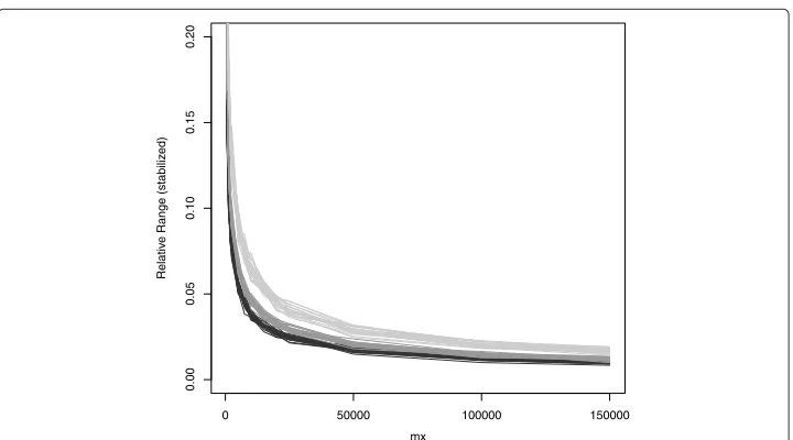
4.3 Number of bootstrap samples
When applying the bootstrap, we have to decide on the number m∗ of bootstrap
samples, required to obtain sufficiently precise results in justifiable time, as bootstrap-ping may consume a considerable amount of time for large data sets and/or many
items. First of all, a means is required to summarize the (loss of ) precision whenm∗
decreases. Because it is a common choice to evaluate the test statistic with respect to the 95 %-quantile of the appropriate limiting distribution, we will concentrate on this measure.
Rather than starting a new simulation, we resorted on the vast amount of data already at hand: The original simulation covered 7 sample sizes times 3 item counts times 3
algorithms, which totals in 7× 3× 3 = 63 vectors, each containing m = 200, 000
realizations of the test statistic (5). In order to evaluate the effect of less than 200,000
bootstrap samples (m∗< m), we drew random subsamples of 14 different sizesm∗from
each of the 63 vectors, each repeated 1000 times. For each of these 882 ×1000
sam-ples, we determined the empirical 95 %-quantile, yielding 882 vectors containing 1000
estimates of the quantile under consideration,qˆ.95. (For notational ease, the index will be
The minimum and maximum value per vector would express a worst case appraisal of error to be found in the simulated data sets. However, in order to avoid singular outliers to detract from a more general perspective, the five most extreme values in each direction were averaged, a procedure which can be considered a stabilized minimum and maxi-mum. The difference of these two figures is divided by the corresponding quantile of the according limiting distribution, which makes the measure comparable across all designs. It will be termedrelative range,rr:
rr=
1 5
n
i=n−4qˆ(i)− 15
5
i=1qˆ(i)
χ2 [.95;df]
, (9)
withqˆ(i) denoting the sorted values of the quantile estimates per combination ofn, k,
algorithm, andm∗.
Figure 2 shows the relative range by number of bootstrap replicationsm∗. Two clear
structures are discernible: First, all lines exhibit a (negative) logarithmic shape without exemption, with deviations rapidly decreasing with increasing number of bootstrap
sam-ples. Second, the larger the number of itemsk, the faster the deviations decrease together
with increasingm∗. However, the latter phenomenon is considerably smaller than the first
one.
Due to the clear shape of the curves, we tried to formulate a general model pre-dicting the required number of bootstrap replicates given a desired precision
crite-rion in terms of rr. In order to apply a linear model, the logarithm of the relative
range rr and the negative logarithm of the bootstrap replication number m∗ were
taken. The algorithm was dummy coded (fr serving as reference category) and the
number of variables k and the sample size n were directly entered into the model
equation
y=β0+β1log(m∗)+β2k+β3n+β4[1]fx+β4[2]nv, (10)
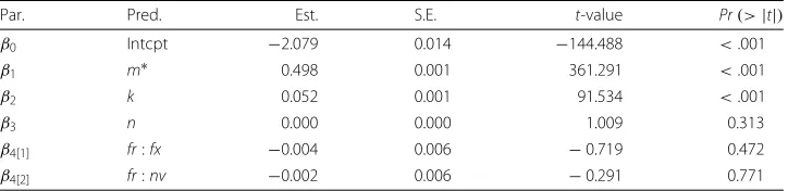
withy= −log(rr)andβ(·)denoting the regression coefficients. Their estimates are given in Table 3 along with the respective significance measures.
The model R2 equalled .994, which indicates a good fit of model (10). Aside of the
intercept β0, the coefficients regarding the bootstrap replication number, β1, and the
number of items,β2, were significantly different from zero, but not those for the sample
size,β3, or the simulation algorithm,β4[·].
This affirms the impression already derived from Fig. 2 thatm∗and (to a much lesser
extent)ksuffice for the determination of the precision of the bootstrap analysis. From the
coefficients indicated in Table 3, a rule of thumb has been developed to obtain a rough estimation of the required number of bootstrap samples (the coefficients were rounded):
m∗=exp 4−0.1k−2 log(rr). (11)
If, for example, one wants to test 8 items with the LRT using two split groups,
then the critical value χ[.95;7]2 = 14.067. The 95 % quantile of the bootstrap
distribu-tion shall not exceed the interval [13, 15] (which complies with the probabilities .964
and .927, respectively), the range is two and the relative range isrr = 2/14.1 = 0.142
(note that the deviations do not behave symmetrically, but this seems negligible in order
to obtain a rough estimation ofm∗). Then, the optimal number of bootstrap replicates
according to (11) amounts to 1219, hence 1200 bootstrap samples will be a good choice.
5 Discussion
The present study focuses on practical issues when applying the Likelihood Ratio statistic according to Andersen (1973) for testing the binary Rasch Model. If the model holds, the Likelihood Ratio test statistic approaches the limiting distribution to a sufficient extent even in cases where samples were small or items were few. The most problematic com-bination of 5 items and 100 observations revealed moderate deviations from the limiting distribution. But even in the most problematic cases the CDFs of the bootstrap and the according limiting distribution differed by no more than 7 %, which seems justifiable to us.
Generally, the approximation of the test statistic under the null-hypothesis shows suf-ficient approximation to the theoretical distribution if samples comprise at least 500 respondents and an instrument with more than ten items is considered. For studies con-sidering smaller samples or fewer items we recommend the more expensive bootstrap method. However, this is little a drawback as bootstrapping small samples takes only a reasonable amount of time. In order to further control the required time, Eq. (11) provides an easily applicable rule of thumb allowing to limit the number of bootstrap samples warranting a precision criterion of interest.
5.1 Size Matters
However, a significance test has its merits as well, as it allows to rely on the decision cri-terion of statistical significance, which is fundamental in scientific reasoning. In order to avoid the propagation of unsubstantiated rules of thumb (cf. Maxwell 2000), a prospective power analysis (in the sense of Cohen 1988) is required. For that purpose, the simulation technique presented here provides a reliable means to obtain the required non-central distributions of the test statistic.
5.2 Simulation technique
In the present study, three pertinent bootstrap algorithms, which we termed normal marginals, free marginals, and fixed marginals method, have been compared. While there was hardly any difference in the null hypothesis cases, some striking differences were encountered for the non-central distributions, deserving further inspection: The LRT
assumes the rowsumsrvto be fixed at their observed values, therefore the fixed marginals
bootstrap adopts this assumption. Any deviation from the observed scores inevitably yields a different likelihood and the sampling distribution of the test statistic will change.
Interestingly, the present study revealed that such a change primarily occurs in the non-central case, which can be explained: If we let the rowsums vary freely (as has been done in the normal marginals and the free marginals case), score frequencies change
as well. Now, in the central case, the same item parameter estimatesβˆ(0) are used for
all subsamples, which supports the assumptions made in the null-hypothesis. But in the non-central case, possibly differing subgroup estimates are used for generating the boot-strap samples. If, say, score group two yields highly deviating estimatesβˆ(2), but the score two has (by chance) only sometimes occurred, the deviation will not be much reflected in the test statistic. But if the same score group would have appeared with a high fre-quency, the deviating estimates will considerably change the product of the subgroup likelihoods in Eq. (4) and the the test statistic will reflect the model violation. Hence, the test statistic (and, in turn, its bootstrap distribution) depends on the relative frequencies of the scores, which explains the observed differences of the three bootstrap methods considered.
Hence, the fixed marginals method has to be considered superior, not only for the theoretical reasons outlined above, but also for the present study revealed in certain cases the differences to be striking. The normal marginals method yielded
problematic distributions of the test statistic (5) when simulating the H1-distribution,
which may also be explained: If we split along the score rv (using the median,
for example), score distributions in the subsamples will inevitably differ, causing the observed differences. Therefore, the normal marginals method is not eligible for that purpose.
5.3 Don’t be naïve!
As has been mentioned above, the naïve bootstrap (i.e. drawing response vectors with replacement from the original sample, cf. Davison and Hinkley 1997) cannot be applied to the present problem: In the specific case of the LRT, this would cause the split group
membership to be drawn at random as well, thus changing the subgroup frequenciesnjof
One might therefore consider to draw the observations separately from the original subsamples. However, this would not yield the desired results: Only the response patterns of the possibly differing subgroup members form each group then, hence we end up with the distribution of the test statistic under the alternative hypothesis.
5.4 Subgroup frequencies
The similarities of the three algorithms in theH0-case could be traced back to the fact that
the original samplesX0have been generated withθ ∼N(0, 1): All bootstrap procedures
reproduced the marginals’ distributions exceptionally well, what will not be necessar-ily the case in a practical application. Hence, we should not use the free or the normal marginals method but the fixed marginals method to perform a power analysis in the sense of Cohen (1988).
However, this algorithm has far-reaching consequences for further research: If one wanted to perform a power analysis of the LRT by means of a simulation study using the fixed marginals method, he or she would have to consider both the item parameters and the score group frequencies. But unfortunately, we face a technical complication here: In order to vary the sample size seamlessly (which is necessary to obtain the optimal sam-ple size), the relative subgroup frequencies have to be maintained. For twice the original sample (or any other integer multiple), each observation can be drawn twice (or three
times, and so on). But for any other sample size, the relative frequenciesnj/nwould have
to be carefully approximated, allowing for a sufficient reproduction of the marginals with increasingn.
5.5 How many bootstrap samples?
One question, which always has to be considered when applying of the bootstrap, is the number of bootstrap replicates that have to be generated. For this purpose, a very gen-eral solution has been found in the present study. Within the parameters considered, the expected maximum deviation of the 95 % quantile of the true distribution can be deter-mined using the number of samples and the number of items. Of course, Eq. (11) could be extended to any other measure of interest, like another quantile, for example. The present approach demonstrated the feasibility of a means to generally determine the required number of bootstrap samples.
5.6 Limitations and outlook
One limitation of the present study can be seen in the fact that only the two groups sample split has been considered. However, the procedure presented here allows for a straightforward extension to any number of split groups. Further, this seems to be only a minor obstactle for the practical application of the present results, as available sample sizes seldom allow for splitting into more than two groups.
the likelihood of the (empirically more restrictive) LLTM is opposed to that of the RM (cf. Alexandrowicz 2011). Again, the methods described here can be adapted accordingly.
The results obtained in the present study have two important implications: First, we are able to obtain the distribution of the test statistic under a fixed alternative by means of the recommended bootstrap method. This allows for determining the required sam-ple size to detect a model violation which is considered relevant from a substantive point of view with fixed risks for the type-I and the type-II errors. And second, the necessary number of bootstrap replications for warranting a desired precision can be obtained. One might object that Eq. (11) only covers up to 15 items and may there-fore not be used for larger instruments. But as we have seen, the larger the number of items, the fewer bootstrap samples are necessary given everything else is held constant. Therefore, one is on the safe side using a minimum of 500 bootstrap samples for data sets comprising more items. The same applies to sample sizes beyond those considered here.
One reason impairing the applicability of the LRT is that the power of the test for a given model deviation could not be determined. As a consequence, no sample planning was possible, leaving the researcher in the dark whether a significant result indicates a model deviation of substantial interest or was merely the consequence of too large a sample. However, this fundamental problem has been overcome by Draxler (2010) for the Wald-test and generalized to the LRT and the Rao-Score-test by Draxler and Alexandrowicz.
These present results allow to determine the optimal sample size required to detect a model deviation considered relevant from a substantial point of view with given risks of an error of the first and the second kind. We believe that the LRT is a valuable tool for testing whether an instrument allows for establishing a measurement and the present findings will facilitate its liable utilization.
6 Conclusion
The test statistic of the conditional Likelihood Ratio Test approximates its limiting dis-tribution very fast. Only the combination of 5 items and 100 respondents revealed slight deviations, however, increasing either the number of items or the sample size will
allow for employing the quantiles of the respectiveχ2-distribution in the usual manner.
Appendix
Table 2Moments and quantiles of the non-central bootstrap distributions
k/df n meth mean var cv skew kurt q50 q90 q95 q99
5/4 100 nv 4.46 9.80 0.70 1.39 2.90 3.75 8.65 10.54 14.70
free 4.65 10.07 0.68 1.31 2.64 4.01 8.89 10.73 14.82
fix 4.72 9.78 0.66 1.24 2.29 4.10 8.92 10.75 14.70
250 nv 50.60 123.32 0.22 0.25 0.02 50.14 65.15 69.58 78.32
free 14.89 27.97 0.36 0.75 0.86 14.19 21.97 24.66 30.01
fix 13.43 23.23 0.36 0.78 0.82 12.66 20.03 22.35 27.03
500 nv 5.07 12.34 0.69 1.34 2.63 4.30 9.81 11.83 16.42
free 4.65 10.64 0.70 1.38 2.87 3.91 9.01 10.95 15.29
fix 4.66 10.75 0.70 1.39 2.87 3.92 9.06 11.02 15.41
750 nv 9.36 29.00 0.58 0.98 1.32 8.45 16.61 19.47 25.63
free 6.77 18.59 0.64 1.16 1.89 5.93 12.61 15.03 20.20
fix 6.77 18.47 0.63 1.15 1.90 5.94 12.58 14.99 19.98
1000 nv 11.61 38.43 0.53 0.89 1.08 10.65 19.97 23.14 29.83
free 8.64 26.15 0.59 1.05 1.57 7.75 15.51 18.34 24.17
fix 8.80 26.28 0.58 1.03 1.50 7.93 15.66 18.47 24.53
2500 nv 9.82 31.20 0.57 1.00 1.46 8.91 17.33 20.24 26.67
free 6.95 19.47 0.63 1.14 1.83 6.10 12.91 15.39 20.71
fix 7.01 19.70 0.63 1.14 1.79 6.15 13.03 15.51 20.78
5000 nv 20.44 73.41 0.42 0.67 0.63 19.49 31.91 35.99 44.45
free 13.48 44.64 0.50 0.82 0.93 12.56 22.48 25.80 32.77
fix 13.95 45.78 0.48 0.79 0.88 13.06 23.05 26.33 33.54
10/9 100 nv 16.63 48.66 0.42 0.76 0.84 15.73 25.98 29.40 36.58
free 16.93 49.66 0.42 0.71 0.67 16.07 26.36 29.88 36.84
fix 17.76 53.02 0.41 0.70 0.66 16.90 27.50 31.02 38.17
250 nv 15.23 43.00 0.43 0.80 0.98 14.37 24.01 27.26 34.21
free 15.23 42.59 0.43 0.78 0.85 14.36 23.97 27.25 34.03
fix 15.83 45.04 0.42 0.77 0.83 14.97 24.82 28.11 35.05
500 nv 24.60 80.08 0.36 0.60 0.47 23.66 36.55 40.73 49.11
free 25.09 82.19 0.36 0.60 0.52 24.17 37.13 41.32 50.00
fix 26.38 88.22 0.36 0.61 0.52 25.42 38.92 43.31 52.47
750 nv 17.83 53.23 0.41 0.73 0.77 16.95 27.59 31.15 38.46
free 18.13 54.32 0.41 0.73 0.76 17.21 28.00 31.63 39.10
fix 18.83 57.38 0.40 0.72 0.77 17.90 28.96 32.67 40.32
1000 nv 19.13 58.74 0.40 0.71 0.71 18.22 29.33 33.11 40.76
free 20.03 62.19 0.39 0.69 0.67 19.13 30.53 34.31 42.26
fix 21.12 66.66 0.39 0.65 0.57 20.24 32.04 35.97 43.88
2500 nv 14.21 38.70 0.44 0.82 0.91 13.34 22.57 25.73 32.28
free 14.47 39.67 0.44 0.80 0.89 13.63 22.97 26.10 32.56
fix 14.96 42.22 0.43 0.80 0.93 14.11 23.64 26.98 33.72
5000 nv 15.19 42.61 0.43 0.79 0.90 14.31 23.92 27.23 33.92
free 15.14 42.54 0.43 0.80 0.92 14.27 23.86 27.15 33.93
fix 15.49 43.84 0.43 0.77 0.76 14.62 24.38 27.65 34.50
15/14 100 nv 21.08 56.32 0.36 0.68 0.66 20.23 31.10 34.73 42.13
free 21.59 58.86 0.36 0.66 0.61 20.74 31.86 35.45 42.99
fix 21.98 59.95 0.35 0.62 0.50 21.15 32.32 35.97 43.36
250 nv 27.02 80.26 0.33 0.60 0.52 26.13 38.94 43.13 51.73
free 28.16 84.17 0.33 0.57 0.44 27.30 40.38 44.68 53.11
Table 2Moments and quantiles of the non-central bootstrap distributions (Continued)
k/df n meth mean var cv skew kurt q50 q90 q95 q99
500 nv 20.85 55.05 0.36 0.66 0.62 20.05 30.72 34.36 41.78
free 20.85 55.55 0.36 0.67 0.64 20.01 30.76 34.34 41.62
fix 21.13 56.11 0.35 0.69 0.71 20.25 31.10 34.78 42.27
750 nv 27.01 80.95 0.33 0.60 0.51 26.08 39.02 43.18 51.58
free 27.86 82.61 0.33 0.59 0.60 27.01 39.87 44.06 52.72
fix 28.37 85.27 0.33 0.58 0.49 27.50 40.65 45.00 53.45
1000 nv 36.14 115.14 0.30 0.49 0.32 35.28 50.30 55.18 65.02
free 37.22 121.78 0.30 0.51 0.34 36.31 51.83 56.89 66.78
fix 38.39 124.94 0.29 0.49 0.35 37.49 53.20 58.22 68.15
2500 nv 24.07 68.46 0.34 0.62 0.54 23.20 35.08 38.98 47.12
free 24.78 71.02 0.34 0.62 0.55 23.90 36.02 39.95 48.09
fix 25.39 73.60 0.34 0.61 0.54 24.51 36.81 40.85 48.82
5000 nv 27.56 81.96 0.33 0.58 0.45 26.69 39.65 43.83 52.29
free 28.52 85.93 0.33 0.56 0.42 27.65 40.82 45.09 53.90
fix 29.17 89.11 0.32 0.58 0.47 28.26 41.71 46.07 55.00
Table 3Coefficients of the linear model predicting the negative log of the relative error from the log of the number of bootstrap samples, the number of items, the sample size and the bootstrap algorithm
Par. Pred. Est. S.E. t-value Pr(>|t|)
β0 Intcpt −2.079 0.014 −144.488 <.001
β1 m∗ 0.498 0.001 361.291 <.001
β2 k 0.052 0.001 91.534 <.001
β3 n 0.000 0.000 1.009 0.313
β4[1] fr:fx −0.004 0.006 −0.719 0.472
and
Draxler
Journal
of
Statistical
Distributions
and
Applications
(2016) 3:2
Page
20
of
25
Table 4Descriptive statistics for the fixed marginals case under the null hypothesis
mean % var % cv % skew % kurt % q50 % q90 % q95 % q99 %
limiting: df=4 4.00 8.00 0.71 1.41 3.00 3.36 7.78 9.49 13.28
k=5/n=100 4.42 10.4 8.86 10.7 0.67 −4.7 1.23 −12.8 2.17 −27.7 3.81 13.5 8.45 8.6 10.17 7.2 13.82 4.1
k=5/n=250 4.19 4.7 8.88 10.9 0.71 0.6 1.39 −1.9 2.74 −8.6 3.47 3.4 8.22 5.7 9.99 5.3 13.91 4.8
k=5/n=500 4.10 2.4 8.53 6.7 0.71 0.9 1.44 1.8 3.10 3.2 3.42 1.9 7.98 2.6 9.81 3.4 13.70 3.2
k=5/n=750 4.06 1.5 8.26 3.3 0.71 0.2 1.43 1.2 3.12 3.9 3.40 1.3 7.90 1.5 9.60 1.2 13.46 1.4
k=5/n=1000 4.02 0.6 8.05 0.7 0.71 −0.3 1.40 −0.7 2.96 −1.3 3.38 0.7 7.81 0.4 9.54 0.6 13.29 0.1
k=5/n=2500 4.02 0.5 8.19 2.3 0.71 0.7 1.43 1.2 3.03 1.2 3.37 0.4 7.83 0.6 9.57 0.9 13.51 1.8
k=5/n=5000 4.00 −0.1 7.99 −0.2 0.71 −0.0 1.43 0.9 3.19 6.4 3.36 0.1 7.76 −0.2 9.47 −0.2 13.14 −1.0
avg. (df=4) 4.12 2.9 8.39 4.9 0.70 −0.4 1.39 −1.5 2.90 −3.3 3.46 3.0 7.99 2.7 9.74 2.6 13.55 2.1
limiting: df=9 9.00 18.00 0.47 0.94 1.33 8.34 14.68 16.92 21.67
k=10/n=100 9.54 6.0 20.05 11.4 0.47 −0.4 0.89 −5.9 1.10 −17.7 8.88 6.4 15.55 5.9 17.87 5.6 22.77 5.1
k=10/n=250 9.14 1.6 18.67 3.7 0.47 0.3 0.95 1.2 1.36 2.3 8.47 1.5 14.93 1.7 17.23 1.8 22.07 1.9
k=10/n=500 9.08 0.9 18.32 1.8 0.47 −0.0 0.95 0.6 1.42 6.4 8.43 1.0 14.80 0.8 17.07 0.9 21.83 0.8
k=10/n=750 9.02 0.2 18.22 1.2 0.47 0.4 0.95 0.3 1.30 −2.6 8.33 −0.2 14.75 0.5 16.97 0.3 21.81 0.7
k=10/n=1000 9.01 0.1 17.93 −0.4 0.47 −0.3 0.94 0.1 1.37 2.8 8.34 −0.0 14.69 0.0 16.92 0.0 21.64 −0.1
k=10/n=2500 9.02 0.2 17.97 −0.2 0.47 −0.3 0.93 −1.1 1.26 −5.5 8.36 0.2 14.73 0.3 16.95 0.2 21.48 −0.9
k=10/n=5000 9.01 0.1 17.87 −0.7 0.47 −0.5 0.93 −0.9 1.30 −2.3 8.37 0.3 14.69 0.0 16.88 −0.2 21.65 −0.1
avg. (df=9) 9.12 1.3 18.43 2.4 0.47 −0.1 0.93 −0.8 1.30 −2.4 8.45 1.3 14.88 1.3 17.13 1.2 21.89 1.1
limiting: df=14 14.00 28.00 0.38 0.76 0.86 13.34 21.06 23.68 29.14
k=15/n=100 14.60 4.3 30.69 9.6 0.38 0.4 0.75 −1.2 0.79 −7.8 13.92 4.4 21.99 4.4 24.74 4.5 30.52 4.7
k=15/n=250 14.13 1.0 28.75 2.7 0.38 0.4 0.77 2.1 0.92 7.0 13.45 0.8 21.28 1.0 23.91 1.0 29.53 1.3
k=15/n=500 14.07 0.5 27.84 −0.6 0.37 −0.8 0.74 −2.0 0.78 −9.4 13.40 0.5 21.15 0.4 23.73 0.2 29.26 0.4
k=15/n=750 14.03 0.2 28.39 1.4 0.38 0.5 0.77 2.3 0.95 10.3 13.36 0.2 21.16 0.5 23.82 0.6 29.26 0.4
k=15/n=1000 14.04 0.3 28.44 1.6 0.38 0.5 0.77 2.0 0.92 7.5 13.37 0.2 21.11 0.2 23.79 0.4 29.49 1.2
k=15/n=2500 14.02 0.2 28.19 0.7 0.38 0.2 0.75 −0.9 0.78 −9.4 13.35 0.1 21.13 0.3 23.76 0.3 29.25 0.4
k=15/n=5000 14.01 0.0 28.06 0.2 0.38 0.1 0.75 −0.4 0.83 −3.3 13.34 0.0 21.09 0.1 23.70 0.1 29.15 0.0
and
Draxler
Journal
of
Statistical
Distributions
and
Applications
(2016) 3:2
Page
21
of
25
Table 5Descriptive statistics for the free marginals case under the null hypothesis
mean % var % cv % skew % kurt % q50 % q90 % q95 % q99 %
limiting: df=4 4.00 8.00 0.71 1.41 3.00 3.36 7.78 9.49 13.28
k=5/n=100 4.38 9.6 9.11 13.8 0.69 −2.6 1.29 −8.9 2.43 −18.8 3.76 12.0 8.43 8.4 10.18 7.3 14.10 6.2
k=5/n=250 4.16 4.1 8.76 9.6 0.71 0.5 1.39 −1.5 2.77 −7.7 3.47 3.4 8.16 4.9 9.98 5.2 13.81 4.0
k=5/n=500 4.08 2.0 8.35 4.4 0.71 0.2 1.41 −0.2 2.93 −2.3 3.42 1.9 7.97 2.4 9.71 2.3 13.58 2.3
k=5/n=750 4.03 0.8 8.16 2.0 0.71 0.2 1.43 1.4 3.16 5.5 3.39 1.0 7.84 0.8 9.52 0.3 13.46 1.4
k=5/n=1000 4.03 0.7 8.09 1.2 0.71 −0.2 1.38 −2.1 2.85 −4.8 3.38 0.7 7.87 1.2 9.55 0.7 13.27 −0.1
k=5/n=2500 4.01 0.1 7.95 −0.6 0.70 −0.5 1.39 −1.9 2.84 −5.4 3.36 0.1 7.78 0.0 9.46 −0.3 13.27 −0.0
k=5/n=5000 4.00 0.1 8.01 0.1 0.71 −0.1 1.44 2.1 3.28 9.2 3.37 0.4 7.79 0.1 9.47 −0.2 13.29 0.1
avg. (df=4) 4.10 2.5 8.35 4.4 0.71 −0.4 1.39 −1.6 2.89 −3.5 3.45 2.8 7.98 2.5 9.70 2.2 13.54 2.0
limiting: df=9 9.00 18.00 0.47 0.94 1.33 8.34 14.68 16.92 21.67
k=10/n=100 9.53 5.9 20.14 11.9 0.47 −0.1 0.92 −2.0 1.27 −5.0 8.86 6.2 15.54 5.8 17.89 5.7 22.82 5.3
k=10/n=250 9.14 1.5 18.51 2.8 0.47 −0.1 0.95 0.7 1.36 2.2 8.47 1.5 14.90 1.5 17.16 1.4 22.05 1.8
k=10/n=500 9.04 0.4 18.04 0.2 0.47 −0.3 0.93 −1.5 1.29 −3.6 8.40 0.7 14.70 0.1 16.91 −0.1 21.75 0.4
k=10/n=750 9.05 0.6 18.13 0.7 0.47 −0.2 0.93 −1.5 1.26 −5.5 8.38 0.4 14.78 0.7 16.97 0.3 21.68 0.1
k=10/n=1000 9.00 0.0 18.02 0.1 0.47 0.0 0.95 0.5 1.34 0.7 8.34 −0.0 14.70 0.1 16.94 0.1 21.66 −0.0
k=10/n=2500 9.03 0.3 18.23 1.3 0.47 0.4 0.95 0.4 1.36 1.8 8.38 0.4 14.70 0.1 17.02 0.6 21.80 0.6
k=10/n=5000 9.02 0.2 18.08 0.5 0.47 −0.0 0.96 1.7 1.39 3.9 8.37 0.3 14.71 0.2 16.98 0.4 21.82 0.7
avg. (df=9) 9.12 1.3 18.45 2.5 0.47 −0.0 0.94 −0.2 1.32 −0.8 8.46 1.4 14.86 1.2 17.12 1.2 21.94 1.3
limiting: df=14 14.00 28.00 0.38 0.76 0.86 13.34 21.06 23.68 29.14
k=15/n=100 14.58 4.2 30.67 9.5 0.38 0.5 0.76 0.8 0.85 −0.3 13.88 4.1 21.98 4.3 24.74 4.5 30.43 4.4
k=15/n=250 14.15 1.1 28.51 1.8 0.38 −0.1 0.76 0.2 0.85 −0.8 13.49 1.1 21.27 1.0 23.91 1.0 29.56 1.4
k=15/n=500 14.05 0.4 28.17 0.6 0.38 −0.1 0.77 2.0 0.94 9.7 13.39 0.4 21.14 0.4 23.76 0.3 29.31 0.6
k=15/n=750 14.03 0.2 27.91 −0.3 0.38 −0.4 0.74 −2.6 0.78 −9.4 13.37 0.2 21.11 0.2 23.66 −0.1 29.11 −0.1
k=15/n=1000 14.03 0.2 27.86 −0.5 0.38 −0.5 0.75 −0.7 0.84 −2.0 13.38 0.3 21.11 0.2 23.67 −0.1 29.04 −0.3
k=15/n=2500 14.01 0.1 28.04 0.1 0.38 −0.0 0.77 1.9 0.88 2.2 13.35 0.1 21.09 0.1 23.75 0.3 29.25 0.4
k=15/n=5000 14.02 0.2 28.19 0.7 0.38 0.2 0.77 1.6 0.89 4.4 13.34 0.0 21.09 0.1 23.76 0.3 29.23 0.3
and
Draxler
Journal
of
Statistical
Distributions
and
Applications
(2016) 3:2
Page
22
of
25
Table 6Descriptive statistics for the normal marginals case under the null hypothesis
mean % var % cv % skew % kurt % q50 % q90 % q95 % q99 %
limiting: df=4 4.00 8.00 0.71 1.41 3.00 3.36 7.78 9.49 13.28
k=5/n=100 4.11 2.7 8.46 5.8 0.71 0.1 1.42 0.7 3.04 1.2 3.45 2.8 7.98 2.6 9.79 3.2 13.66 2.9
k=5/n=250 4.04 1.0 8.19 2.4 0.71 0.2 1.43 1.4 3.14 4.7 3.39 1.0 7.86 1.0 9.60 1.2 13.43 1.2
k=5/n=500 4.02 0.6 8.09 1.2 0.71 0.0 1.42 0.3 3.04 1.2 3.37 0.4 7.82 0.5 9.53 0.4 13.34 0.5
k=5/n=750 4.01 0.3 8.04 0.5 0.71 −0.1 1.41 −0.2 2.98 −0.6 3.37 0.4 7.80 0.3 9.50 0.1 13.35 0.6
k=5/n=1000 4.02 0.4 8.05 0.6 0.71 −0.1 1.41 −0.6 2.93 −2.2 3.37 0.4 7.80 0.3 9.51 0.2 13.30 0.2
k=5/n=2500 4.00 0.1 8.03 0.4 0.71 0.1 1.44 1.8 3.16 5.2 3.35 −0.2 7.79 0.1 9.48 −0.1 13.33 0.4
k=5/n=5000 4.03 0.6 8.12 1.5 0.71 0.1 1.41 −0.2 2.98 −0.8 3.39 1.0 7.83 0.6 9.54 0.6 13.30 0.2
avg. (df=4) 4.03 0.8 8.14 1.8 0.71 0.0 1.42 0.5 3.04 1.2 3.38 0.8 7.84 0.8 9.56 0.8 13.39 0.9
limiting: df=9 9.00 18.00 0.47 0.94 1.33 8.34 14.68 16.92 21.67
k=10/n=100 9.20 2.2 18.86 4.8 0.47 0.1 0.95 0.3 1.32 −0.6 8.52 2.1 15.02 2.3 17.30 2.3 22.15 2.2
k=10/n=250 9.05 0.6 18.12 0.7 0.47 −0.2 0.92 −2.3 1.25 −5.9 8.41 0.8 14.77 0.6 16.98 0.4 21.64 −0.1
k=10/n=500 9.06 0.7 18.25 1.4 0.47 0.0 0.95 0.5 1.32 −1.2 8.38 0.4 14.78 0.7 17.01 0.5 21.86 0.9
k=10/n=750 9.02 0.3 18.16 0.9 0.47 0.2 0.95 0.5 1.42 6.8 8.37 0.3 14.72 0.2 16.95 0.2 21.67 0.0
k=10/n=1000 8.99 −0.1 17.86 −0.8 0.47 −0.3 0.94 −0.3 1.32 −1.2 8.33 −0.2 14.68 −0.0 16.88 −0.2 21.57 −0.4
k=10/n=2500 9.01 0.2 18.05 0.3 0.47 −0.0 0.95 0.8 1.39 4.4 8.38 0.4 14.68 −0.0 16.92 0.0 21.70 0.2
k=10/n=5000 9.01 0.1 18.03 0.2 0.47 0.0 0.95 0.9 1.37 3.0 8.34 −0.0 14.66 −0.2 16.96 0.2 21.71 0.2
avg. (df=9) 9.05 0.6 18.19 1.1 0.47 −0.0 0.94 0.1 1.34 0.8 8.39 0.5 14.76 0.5 17.00 0.5 21.76 0.4
limiting: df=14 14.00 28.00 0.38 0.76 0.86 13.34 21.06 23.68 29.14
k=15/n=100 14.32 2.3 29.30 4.7 0.38 0.0 0.76 0.2 0.87 1.4 13.65 2.3 21.53 2.2 24.20 2.2 29.88 2.5
k=15/n=250 14.09 0.7 28.27 1.0 0.38 −0.2 0.76 0.6 0.90 4.8 13.45 0.8 21.20 0.6 23.82 0.6 29.22 0.3
k=15/n=500 14.05 0.4 28.33 1.2 0.38 0.2 0.75 −1.1 0.82 −4.4 13.40 0.5 21.19 0.6 23.80 0.5 29.16 0.1
k=15/n=750 14.00 −0.0 27.85 −0.5 0.38 −0.2 0.73 −3.9 0.72 −15.8 13.35 0.1 21.09 0.1 23.65 −0.1 28.88 −0.9
k=15/n=1000 14.07 0.5 28.40 1.4 0.38 0.2 0.77 2.1 0.91 6.3 13.42 0.6 21.16 0.5 23.84 0.7 29.50 1.2
k=15/n=2500 14.04 0.3 28.30 1.1 0.38 0.3 0.77 2.5 0.99 15.4 13.39 0.4 21.08 0.1 23.77 0.4 29.37 0.8
k=15/n=5000 14.02 0.1 28.10 0.4 0.38 0.0 0.75 −0.6 0.83 −3.3 13.37 0.2 21.07 0.0 23.73 0.2 29.20 0.2
Table 7Kolmogorov-Smirnov test for fit to the limiting distribution
fix free nv
k n D p D p D p
5 100 0.0700 <0.0001 0.0608 <0.0001 0.0155 <0.0001
5 250 0.0256 <0.0001 0.0212 <0.0001 0.0063 <0.0001
5 500 0.0127 <0.0001 0.0108 <0.0001 0.0039 0.0052
5 750 0.0087 <0.0001 0.0071 <0.0001 0.0033 0.0241
5 1000 0.0063 <0.0001 0.0062 <0.0001 0.0040 0.0037
5 2500 0.0036 0.0123 0.0033 0.0288 0.0037 0.0096
5 5000 0.0028 0.0842 0.0038 0.0060 0.0061 <0.0001
10 100 0.0521 <0.0001 0.0499 <0.0001 0.0188 <0.0001
10 250 0.0135 <0.0001 0.0139 <0.0001 0.0072 <0.0001
10 500 0.0093 <0.0001 0.0076 <0.0001 0.0061 <0.0001
10 750 0.0043 0.0013 0.0061 <0.0001 0.0046 0.0005
10 1000 0.0037 0.0074 0.0019 0.4893 0.0028 0.0971
10 2500 0.0035 0.0150 0.0061 <0.0001 0.0044 0.0007
10 5000 0.0044 0.0009 0.0039 0.0044 0.0027 0.1048
15 100 0.0447 <0.0001 0.0421 <0.0001 0.0243 <0.0001
15 250 0.0104 <0.0001 0.0126 <0.0001 0.0088 <0.0001
15 500 0.0079 <0.0001 0.0060 <0.0001 0.0060 <0.0001
15 750 0.0048 0.0002 0.0042 0.0017 0.0026 0.1301
15 1000 0.0049 0.0001 0.0043 0.0011 0.0069 <0.0001
15 2500 0.0028 0.0926 0.0026 0.1269 0.0054 <0.0001
Table 8Thep-values of the theoretical quantiles applied to the bootstrap distributions
α=.10 α=.05 α=.01
n k=5/df=4 nv free fix nv free fix nv free fix
100 p-value 0.11 0.13 0.13 0.06 0.07 0.07 0.01 0.01 0.01
rel. err. 8 % 28 % 30 % 13 % 32 % 33 % 18 % 41 % 28 %
250 p-value 0.10 0.12 0.12 0.05 0.06 0.06 0.01 0.01 0.01
rel. err. 3 % 16 % 18 % 5 % 21 % 22 % 6 % 25 % 30 %
500 p-value 0.10 0.11 0.11 0.05 0.06 0.06 0.01 0.01 0.01
rel. err. 2 % 7 % 8 % 2 % 10 % 13 % 3 % 13 % 21 %
750 p-value 0.10 0.10 0.11 0.05 0.05 0.05 0.01 0.01 0.01
rel. err. 1 % 3 % 5 % 1 % 2 % 4 % 3 % 9 % 8 %
1000 p-value 0.10 0.10 0.10 0.05 0.05 0.05 0.01 0.01 0.01
rel. err. 1 % 4 % 1 % 1 % 3 % 2 % 1 % 0 % 1 %
2500 p-value 0.10 0.10 0.10 0.05 0.05 0.05 0.01 0.01 0.01
rel. err. 0 % 0 % 2 % 0 % −1 % 3 % 2 % 0 % 11 %
5000 p-value 0.10 0.10 0.10 0.05 0.05 0.05 0.01 0.01 0.01
rel. err. 3 % 1 % −1 % 3 % 0 % −1 % 1 % 1 % −6 %
k=10/df=9
100 p-value 0.11 0.13 0.13 0.06 0.07 0.07 0.01 0.02 0.02
rel. err. 10 % 27 % 27 % 13 % 34 % 34 % 20 % 52 % 46 %
250 p-value 0.10 0.11 0.11 0.05 0.05 0.06 0.01 0.01 0.01
rel. err. 3 % 6 % 7 % 3 % 8 % 10 % −1 % 14 % 15 %
500 p-value 0.10 0.10 0.10 0.05 0.05 0.05 0.01 0.01 0.01
rel. err. 3 % 0 % 4 % 3 % 0 % 5 % 8 % 3 % 6 %
750 p-value 0.10 0.10 0.10 0.05 0.05 0.05 0.01 0.01 0.01
rel. err. 1 % 3 % 2 % 1 % 2 % 2 % 1 % 1 % 6 %
1000 p-value 0.10 0.10 0.10 0.05 0.05 0.05 0.01 0.01 0.01
rel. err. 0 % 1 % 0 % −1 % 1 % 0 % −3 % 0 % −1 %
2500 p-value 0.10 0.10 0.10 0.05 0.05 0.05 0.01 0.01 0.01
rel. err. 0 % 1 % 1 % 0 % 4 % 2 % 1 % 5 % −5 %
5000 p-value 0.10 0.10 0.10 0.05 0.05 0.05 0.01 0.01 0.01
rel. err. −1 % 1 % 0 % 1 % 2 % −1 % 1 % 5 % 0 %
k=15/df=14
100 p-value 0.11 0.12 0.13 0.06 0.07 0.07 0.01 0.02 0.02
rel. err. 12 % 24 % 25 % 15 % 31 % 32 % 25 % 47 % 49 %
250 p-value 0.10 0.11 0.11 0.05 0.05 0.05 0.01 0.01 0.01
rel. err. 3 % 5 % 6 % 4 % 7 % 6 % 2 % 14 % 12 %
500 p-value 0.10 0.10 0.10 0.05 0.05 0.05 0.01 0.01 0.01
rel. err. 3 % 2 % 2 % 3 % 2 % 1 % 1 % 5 % 4 %
750 p-value 0.10 0.10 0.10 0.05 0.05 0.05 0.01 0.01 0.01
rel. err. 1 % 2 % 2 % −1 % −1 % 4 % −5 % −1 % 5 %
1000 p-value 0.10 0.10 0.10 0.05 0.05 0.05 0.01 0.01 0.01
rel. err. 2 % 1 % 1 % 4 % −1 % 4 % 11 % −2 % 9 %
2500 p-value 0.10 0.10 0.10 0.05 0.05 0.05 0.01 0.01 0.01
rel. err. 0 % 1 % 2 % 2 % 2 % 2 % 7 % 3 % 3 %
5000 p-value 0.10 0.10 0.10 0.05 0.05 0.05 0.01 0.01 0.01
rel. err. 0 % 1 % 1 % 1 % 2 % 0 % 2 % 2 % 0 %