Image offset density distribution model and recognition of hand knuckle

R E S E A R C H

Open Access

Image offset density distribution model

and recognition of hand knuckle

Shiqiang Yang

, Luqi Gong and Dan Qiao

Abstract

The accurate description of hand posture plays an important role in the man-machine interaction involved in coordinated assembly. Knuckle image extraction and recognition are of great significance to refine and enrich hand-pose information. These are based on nonparametric density kernel estimation observation sets

corresponding to unilateral and bilateral excursion of the hand knuckle gray image. In this paper, sets of pixel positions belonging to the upper- and middle-density intervals are used as two types of image targets. Random clustering and random field multi-classification target modeling are used to learn and estimate the two target distributions of the image. The discriminant field classification learning method is used to fuse the two kinds of target models. A comprehensive representation of the image offset features is obtained. Finally, the knuckle image sample set is used to train the model, and the adaptive threshold is used to identify the hand knuckle image. The results show that the proposed method is feasible.

Keywords:Knuckle recognition, Image offset density, Gaussian process, Infinite Dirichlet process

1 Introduction

In intelligent manufacturing systems, the development of detection technology with high intelligence and strong en-vironmental adaptability is of great significance to improve production efficiency and enhance the flexibility of manu-facturing systems and product quality [1, 2]. Machine vision-based human-computer interaction coordination assembly technology uses human assembly gestures ob-tained from image analysis as input information for robot task planning [3] to realize an efficient and flexible coordi-nated assembly process [4]. The overall information, in-cluding the biological structure of the human hand image and associated hand assembly posture [5], is the basis for inferring the gesture intention.

Gesture-recognition research has two main directions. One uses sensors, detectors, and other peripheral tools to achieve gesture recognition. Lee and You [6] identified complex static gestures using wrist band-based contour fea-tures (WBCFs). The user must wear black wristbands to ac-curately segment the hand area. Moschetti et al. [7] recognized nine gestures with inertial sensors placed on the

index finger and wrist. This kind of method, which uses external equipment to extract the hand position and pos-ture to achieve more accurate gespos-ture recognition, lacks convenience. Another research direction is unmarked ges-ture recognition with capges-tured images. Bao et al. [8] classi-fied images of gestures using deep convolutional neural networks. This method requires no segmentation or detec-tion to distinguish irrelevant non-hand regions. Dehankar et al. [9] used accurate end-point identification (AEPI) to recognize hand-gesture images against varying backgrounds and blurred images. However, the above unmarked gesture-recognition methods are not sufficiently accurate. Their robustness and stability are insufficient, and the pose cannot be completely extracted. Further research is needed to improve their ability to accurately extract hand positions. Many new identification technologies have emerged in the field of image-feature detection. These methods are used in different fields and vary in their focus. Some focus on feature-extraction techniques. Ding et al. [10] used double local binary patterns (DLBPs) to detect frame peaks in video. Yao et al. [11] presented a feature-selection method based on filters. Some have focused on model building, such as Wang and Wang [12], who modeled an action class of body space configuration with flexible quantities. A hierarchical spatial SPN method was developed to simulate the spatial

* Correspondence:[email protected]

School of Mechanical and Precision Instrument Engineering, Xi_’an University of Technology, 5 South Jinhua Road, Xi’an, Shaanxi Province 710048, People’s Republic of China

relationships among sub-images, and sub-image correlation was modeled by additional layers of the SPN. Panda et al. [13] proposed a feature-driven selection classification algo-rithm (FALCON) to optimize the energy efficiency of machine-learning classifiers. The study of feature clustering is helpful for image-feature classification. Li et al. [14] used an unsupervised principal component analysis (PCA)-based fea-ture clustering algorithm to automatically select the optimal number of clusters to solve the problem of automatic anom-aly detection in monitoring applications. Jiang et al. [15] pro-posed a self-organizing feature clustering algorithm based on fuzzy similarity to extract text features. This method is fast and can extract features better than other methods. Rahmani and Akbarizadeh [16] proposed a spectral clustering method using unsupervised feature learning (UFL).

There is a strong correlation between the structured in-formation of the hand image and the biological structure of the hand. The specific structural information varies with the gesture model, depending on the simplified bio-logical structure. Under static conditions, vision-based gesture-structure modeling is mainly classified as either feature template representation based on two-dimensional models or hand geometry representation based on three-dimensional models, depending on the dimension of the investigated spatial domain [17,18]. The latter is di-vided into a volumetric model that considers the surface structure of the hand [19] and a joint-linking model that considers the anatomy of the hand, according to the estab-lished differences in the geometric characteristics [20]. The template-based modeling is characterized by gesture-contour information, which makes it difficult to provide detailed kinematic parameter information, and is suitable for scenes where the gesture is simple and the se-mantic features are clear. For complex situations in which the hand posture is variable, semantic features and time are related, and the structural parameters of the “join-t-link” model of the hand are modeled. The overall kine-matic representation of the hand can be obtained through structural parameter detection.

The biometric identification of the hand includes skin-color location, fingertip root detection [21], knuckle recognition, finger positioning, and kinematic correlation between features. The knuckle position feature has an im-portant influence on the accuracy of the opponent-pose inference. Knuckle image detection methods are mainly classified as geometric analysis or texture recognition [22–24]. Current research of knuckle images focuses on the use of knuckles for identification, sometimes com-bined with fingerprints. The way and purpose of its re-search is similar to fingerprint detection [25]. Usha and Ezhilarasan [26] used feature-extraction methods based on angle geometry analysis (AGFEM) and contourlet transform (CTFEM) to authenticate the finger back sur-face (FBKS) [27], and pointed out that the distal

phalangeal region of FBKS, the finger joint area near the tip of the finger, has great potential for recognition. Recog-nition performance is improved through extraction and integration of knuckle geometry and texture features sim-ultaneously with fractional fusion. Lin et al. [28] provided a practical solution for biometric systems based on the back of the finger through the FKP recognition algorithm. Gao et al. [29] used an adaptive binary fusion rule to adap-tively fuse the matching distances before and after recon-struction, reducing false-rejection rate. Kumar and Xu [30] used an automatic finger-recognition study of the lowest finger joint pattern formed between the metacarpal and the proximal phalange.

Image segmentation based on a skin-color model can ini-tially solve the problem of image-positioning in the hand. The important image features that characterize the biological structure of the hand, such as finger posture and knuckle position, still must be further identified. The human finger section is the important positioning point for the human hand posture. Gesture recognition requires accurate knuckle position information for three-dimensional reconstruction to restore the hand biostructure. In the half- and full-grip pos-tures of the hand, corresponding to the joint structure at the joint position of the hand, the grayscale distribution of the knuckle image presents an irregular convex-hull structure near the local position of the finger. A non-deterministic ir-regular convex hull can be used as a kind of random hidden structure of knuckle images. In a previous article [31], the author took a finger joint image as an example. The exam-ples are directed to a random image with the above gray structure ambiguity, feature ambiguity, and difficulty in extraction. The hidden feature observation of the image is obtained by the density estimation of the gray distribution. This observation is used to establish the framework of learn-ing and estimatlearn-ing algorithms for imagery-implicit feature patterns. The extraction and analysis methods of the offset features on random images are given.

In this paper, the human-computer interaction is coor-dinated and assembled in an indoor environment where the light intensity is relatively stable and the camera angle is relatively fixed. The research in this paper is based on the image offset density distribution. First, the image upper level density feature is modeled and ana-lyzed with an infinite Dirichlet process model. Then, the image middle-density feature is modeled and analyzed with a Gaussian process classifying model. Finally, the two-level density features are fused by a binary Gaussian process classification. Experiments are carried out to verify the feasibility of the process.

2 Infinite Dirichlet process knuckle image high-level data hybrid model

test imageAin the random image grayscale distribution model is

^

μ≈D ~μG1jℙ

0

δ _~μ

ℙj0;c1

ð Þ;μ~G1jℙ

0

δ _~μ

ℙj0;c21;c22

ð Þ

; ð1Þ

whereμ^is the approximation form of the offset meas-ure,Dis the fusion structure between different offset set models under different offset parameters, ~μ_G1jℙ0 is the high-level offset set probability measure, and~μ_G2jℙ

0 is the middle offset set probability measure.

For ease of calculation and presentation, the condi-tional random measure is expressed as

pð Þ ∝~μ_G1jℙ0ð Þ; ð2Þ

where p(⋅) is the non-negative two-dimensional dens-ity function corresponding to the target distribution.

For the learning problem of unilateral offset density in image stochastic models, this section uses an infinite Dirichlet process hybrid model. Based on the gray-level position data extracted from the nonparametric density kernel estimation results, the probability measure ~μ_G1jℙ0 of the offset set belonging to the fixed thresholdcin the image domain is learned. The number of clusters is de-scribed as a random state, and the Gibbs sampling method is used to iteratively study the density structure of the hierarchical probability form under the assump-tion of the Markov neighborhood. Through learning and modeling the offset set distribution, the unilateral esti-mation of the gray particle random model is realized.

2.1 Horizontal density clustering and Markov assumptions for discrete observations

In the layered observations of the density estimate fK, the process of determining the positions of the unilat-erally offset grid points that belong to the horizontal parameter cis equivalent to the marking process on the discrete grid points of the image:

V¼ ðx;yÞ∈Zjf_Kððx;yÞ;tXÞ= max Z fK

≥c;c>0

ð3Þ

Z¼V∪ðZnVÞ: ð4Þ

Among them, the marker amount constitutes a hidden variable at the observation grid Z. To learn the distribu-tion model of the observadistribu-tions by using observadistribu-tions, the relationship between observations, label classes, and offset measures on grid Z must be established. OnVand

Z\V, respectively, the position in the observed set V has a definite marker class 1 on the image. However, the la-beling category Z\V on the unobserved position set is uncertain. Under the assumption of the continuity of the

distribution model, the position where the marker cat-egory is indefinite should be understood as not observed, and the 0 marker cannot directly determine the corre-sponding observation result. The label category indicates whether the observation position belongs to the offset set under the level c. However, when estimating the overall offset measure using the observation data, it is necessary to further specify the mark relationship be-tween the elements of the sets V and Z\V to integrate the mark relationships on the entire grid point Z. In connection with the data-extraction process in the previ-ous article [30], the dependency relationship between grid observations can be established on Z using the mix-ture graph strucmix-ture as a basis for subsequent inference learning using observation data. The relationship be-tween marker categories and grid positions is established through a directed graph structure. At the same time, pairwise Markov random fields are used to establish a dependency relationship between the discrete grid points on the imaging domain, i.e., the distribution ofp(⋅) onZ. Thus, the hidden Markov model with observation markers is constructed on the grid point Z, as shown in Fig.1. Among them, the hidden variable is the mark type, and the correlation factor is the local dependency on the offset set. The observations extracted based on the density estimate have neighborhood structures similar to those observed in the original grayscale image. Therefore, the corresponding semanticp(⋅) on the grid pointZnot only forms a meaning on the image as a whole but also has a dependency in the local area and is a local Markov hy-pothesis on the corresponding undirected graph model:

p xi∈VjxZni

¼p x i∈VjxΓð Þi : ð5Þ

That is to say, observations that depend on the overall distribution are separated from the whole in the form of local associations.

According to the above analysis, on the one hand, the offset measure on the random hyperparameter fieldf re-flects the characteristics of the observation mark classifi-cation and the density distribution agglomeration under the local relation. On the other hand, considering that when the offset set level parameter is higher, the Euler indicative number of the offset set is larger, and it shows that the local coverage of the offset set at the high level in the planar domain is more complete and shows more of a clustering trend. Therefore, the learning problem for p(⋅) can be transformed to a random clustering

structure of the hierarchical probability form under the assumption of the Markov neighborhood.

2.2 Nonparametric distributions and infinite Dirichlet processes

To improve the adaptability of the model to the target distribution, the model of the target distribution p is represented as a nonparametric hybrid model,

p xτð Þ1;xτð Þ2;…;xτð ÞN

¼

Z

Θ

pð Þθ Y N

i¼1

p xð ijθÞdθ; ð6Þ

whereθ is a hyperparameter, which is not limited to a limited form of distribution to improve the learning ef-fectiveness and image-recognition rate.

In particular, the Dirichlet process defines the distribution of stochastic components on a stochastic probability meas-ure as an effective alternative to parametric model learning. The nonparametric method constructs a stochastic process on the infinite dimensional parameter spaceΘand quanti-fies it by the finite statistics of the stochastic process, where

Θis the measurable space. The Dirichlet process is defined by the base measure H onΘand the central parameterα.

Θ'

slimited distribution(T1, …,Tk) is:

∪K

k¼1Tk¼Θ; Tk∩Tl¼∅;k≠l ð7Þ

The mean of the random probability distributionGon

Θ over the finite-match diversityTfollows the Dirichlet distribution:

G Tð Þ1 ;…;G Tð Þk

ð Þ DirðαH Tð Þ1 ;…;αH Tð Þk Þ: ð8Þ

The random processDP(α,H) is defined by the central parameterαand the base measureH.

Since the parameterαcontrols the probability distribution of random parameter sets in the Dirichlet process, the later update and accurate sampling have a decisive effect on the convergence of iterative learning. Since the sampling strategy ofαis related to the generation mechanism of the random measure distribution in the Dirichlet process, the sampling details corresponding to different generation mechanisms differ slightly. In this section, under the idea of discrete approximation based on lattice Gibbs mixed sampling, the prior distribution is taken as the Gamma distribution,

α∼G að ;bÞ: ð9Þ

The posterior condition update form using a multi-gamma distribution mixing representation (taking a mix number of 2) is

αjη;k

ð Þ∼πηG að þk;b−logð ÞηÞ

þ1−π_ηG að þk−1:b−logð ÞηÞ;

ð10Þ

where G is the Gamma distribution, Kis the current number of updated clusters in the Dirichlet blending process (DPMM), andnis the observed data volume,

η∼Betaðαþ1;nÞ ð11Þ

πη¼ aþK−1

aþK−1þnðb−logð ÞηÞ: ð12Þ

mean of the above conditional distribution is taken as the final sampling result:

pðαjDnÞ≈N−1 XN

s¼1p αjηs;ks

; ð13Þ

whereN is the number of samples and ksmay have a degeneration value ofK.

For the intra-group parameters, the specific components of the image offset set target distribution can adopt a two-dimensional Gaussian distribution. In order to make the update law of Gaussian distribution, parameters meet the requirements of a posteriori maximization. For the two quantities to be learned, namely the mean parameter and the covariance, the normal-Inverse-Wishart distribu-tion [32] can be taken as the conjugate form of the corre-sponding joint edge distribution. The posterior update law of its parameters is:

μn¼ K0 K0þn μ0

þ n

K0þn x

Kn¼K0þn vn¼v0þn

Λn¼Λ0þSþ

K0n K0þn

x−μ₀

ð Þðx−μ₀ÞT 8 > > > > > < > > > > > :

ð14Þ

where μ0, Λ0, K0, andν0 are the initialized mean pa-rameters, the scale matrix, the data dimension, and the degree of freedom. Get posterior joint edge distribution:

ρ μ;XjD;μ₀;Κ0;Λ0;ν0

¼NIW μ;Xjμ_n;Κn;Λn;νn

ð15Þ

By sampling the above distribution, an effective clus-tering parameter update can be obtained, and the update learning of parameters in each mixed Gaussian compo-nent can be realized.

2.3 Infinite Dirichlet process mixed model based on collapsed Gibbs sampling

According to theNobservationsx¼ fxigNi¼1of the

Dirich-let process mixed model, the hidden variable label zi, the total number of clusters, and the corresponding parameter fθkgKk¼1 are inferred. The exact posterior distribution p(π, θ|x) contains the distributions corresponding to all possible category labeling spaces, and it uses a collapsed Gibbs sam-pling algorithm to implement iterative learning of an infin-ite clustering mixture model. First, all observed variables are sampled with their corresponding hidden variables zi, then the posterior edgeπof the polynomial corresponding to the current label class distribution and all clustering hyperparametersfθkgKk¼1is calculated.

Fixing the rest of the observation variables of the la-tent variable z\i, the current distribution of the hidden variables of the current measurement is

p z ijzni;x;α;λ∝p z ijzni;αp x ijz;xni;λ: ð16Þ Under the assumption of exchangeable text, the first item in the above formula can be expressed as

p zijzni;α

¼ 1

αþN−1

XK

k¼1N−kiδðzi;kÞ þαδ zi;k

;

ð17Þ

where k represents the cluster label in all current, in-finitely many empty tag categories. Similar to the finite mixture model, the likelihood of observing the fixed class model atxiis

p x ijzi¼k;zni;xni;λ¼p xij xjjzj¼k;j≠i

;λ

:

ð18Þ

Similarly, the predicted likelihood of the current obser-vationxiunder the new markerkis

p xijzi¼k;zni;xni;λ

¼p xð ijλÞ ¼

Z

Θ

f xð ijθÞhðθjλÞdθ;

ð19Þ

whereH(λ) is the specified conjugate prior. The Dirichlet process hybrid model contains infinitely many goals to be learned parameters and generalizes the learning inference of the finite mixture model. The specific flow is as follows:

①The next resample of sample markerzð_itÞis started

with the Dirichlet hyperparametersαð₀t−1Þandzð_it−1Þði

¼1;…;NÞ.

②The random array {1, 2,…,N} of the observation

sequenceτ(⋅) is sampled.

③According to the last iteration, the initialization

parameters are set toz=z(t−1)andα0¼αð0t−1Þ.

④For random arrangementi∈τ(1),…,τ(n):

(a) The observation datax_iare removed from the

marker classz_i, and the sufficient statisticsSziand

nzi of the observation classziare updated.

(b) Ifx_iis the only observation in the current category,

the category label and all corresponding clustering

parameters are cleared. Update statisticsSzi andnzi,

totalK=K−1 of marker class.

(c) Relabel all non-empty activation categories 1,…,K.

(d) Calculate the prediction likelihood for allK-like

clusters that are activated based on the statistics

fSkgKk¼1andfnkgKk¼1: f_kð Þ ¼xi p xij xjjzj¼k;j≠i

;λ

:

f_Kþ1ð Þ ¼xi Z

F xð ijθÞG0ð Þθ dθ:

(e) Sample new class ofzifrom the (K+ 1)-dimensional

polynomial distribution:

zi∼ αfkð Þxi δðzi;kÞ þ XK

k¼1N

−i

k fkð Þxi δðzi;kÞ

=Zi

Zi¼αfkð Þ þxi XK

k¼1N

−i k fkð Þxi ;

where N−_ki is the total number of observations for which the current observation position i belongs to the labelk.

(f ) Ifz_i=K+ 1, a new clustering marker is obtained

and denoted asK+ 1. The new clustering parameter

corresponding to (K+ 1) is sampled byH( _i|x_i).

(g) Update sufficient statisticsfSkgKk¼1andfnkgKk¼1 for

all category markers.

⑤It is judged whether all categories are resampled. If

not, return to the flag u1, and return to①for the next

resampling.

⑥Sample all clustering parameters for all tagged

classes:

θð Þt

k ∼p θkj xijzð Þit ¼k

n o

;λ

:

⑦Sample using the auxiliary variable method:

αGamma að ;bÞ;αð Þ₀t∼pðα0jK;n;a;bÞ:

3 Method—knuckle image mid-level data model

In view of the complexity of the random offset set itself, the difference between the offset characteristics corre-sponding to different offset parameter intervals is rela-tively large. And the further the offset parameter is from the standard value of 1, the more complex the corre-sponding feature. Therefore, in the learning process of random image bilateral offset measurement, especially for the case of small offset parameters, it is necessary to deeply analyze the random distribution characteristics of the actual offset observations in the training image data-base and to select an appropriate model for learning. In

this section, we obtain the ~μ_G2jℙ0 equivalent density esti-mate pðÞ∝~μ_G2jℙ

0

ðÞ by learning the multi-label distribu-tion random field model for the mid-density locadistribu-tion.

3.1 Mid-level data distribution training based on Gaussian process classification

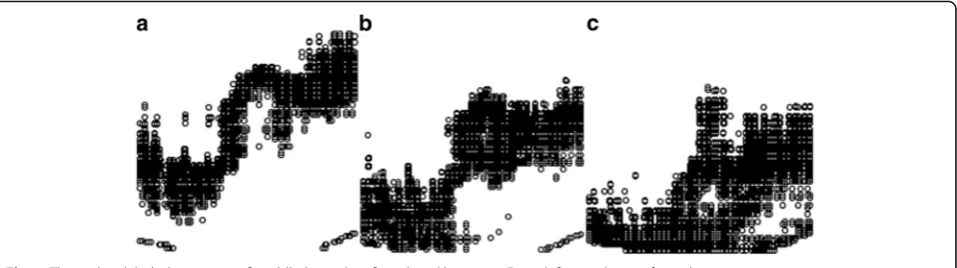
Due to the complexity of the distribution patterns in the middle-level data, it is difficult to obtain a mid-level mi-gration density distribution model with relatively obvious features and a certain resolution. According to the non-parametric density kernel estimation result, the image gray position data corresponding to the offset parameter in the selected interval segment are taken as an observation of the random offset image bilateral offset set. The endpoints of the offset parameter interval are c21= 0.50 and c22= 0.85, and the middle-layer data are further divided into a multilayer structure corresponding to the three types of labels, according to the level of the corresponding density level, as shown in Fig.2. Figure2a–c respectively corres-pond to observations in the intervals 0.70–0.85, 0.60–0.75, and 0.50–0.65. With the decrease of the offset parameter, the distribution pattern in Fig. 2a has certain regression characteristics. Figure 2b shows a clustering trend, and Fig. 2c shows the spread features. Comparing the transi-tions between the three graphs, it can be seen that the mid-level data distribution does not obviously have the clustering patterns or trends implicit in the high-level data distribution. Instead, it reflects the characteristics of ran-dom fields, i.e., the overall distribution of middle-level data, has the transition characteristics from clustering to irregular diffusion. In the above judgment of the distribu-tion characteristics of the mid-level data, a random distri-bution modeling method can be used to learn the typical distribution states of the three parameter segments in the “clustering-diffusion” classification mode and to obtain

~ μG2jℙ

0

transformation of state tags at the same location and the other is the distribution relationship between different locations and multiple states. For the former, the Gibbs form is used to represent the parameter association in the corresponding polynomial distribution of the label. Accounting for the limitations of the complexity of the learning process, this paper assumes that the different tag classes between image locations are irrelevant, and the joint distribution of tags of the same type has Gauss-ian characteristics. The GaussGauss-ian field function fis used to represent tag associations between the same classes:

yc_i j fc_i Bern σ fijyci ¼1

ð20Þ

p yc ijf

c i

¼πc

i ¼σ ycif c i

¼ exp f

c i P

c0 exp f c0 i

; ð21Þ

where the location i tag yc

i has {0, 1} value, and the f vector form is f ¼fðf1₁;…;f1_n;f2₁;…;f2_n;f₁3;…;f3_nÞ. It has a prior form f jX∼N ð0;KÞ, where Kis the corre-sponding covariance function and n is the amount of training data. Assuming the category information is not related, Khas the form of a diagonal matrix, K=diag{

k1,k2, …,kc}, where kc represents the trust relationship between each type of tag data. Therefore, the learning of the middle-level migration measure is transformed to the learning of the random quantityf.

3.2 Posterior calculations on Gaussian fields with multiple binary classifications

Since the fieldfi=f(⋅|xi) is a Gaussian function, the pos-terior form is also Gaussian:

f N^fjf;A−1_{∝ exp −}1

2 f−^f

T

A f −^f

:

ð22Þ

The maximum posterior estimate of the implicit func-tion f is defined as ^f ¼ arg maxfpðfjX;yÞ, A¼−∇∇ logpðf ¼^fjX;yÞ:

Under the Bayesian framework,

p fð jX;yÞ ¼p yð jfÞp fð jXÞ=p yð jXÞ: ð23Þ

Since the classification mark y of test dataset Xis not directly related to f, i.e., p(y|X) does not include f, the posterior maximum solution of fcorresponds to the log likelihood of^f:

Ψð Þf ≜logðp yð jfÞp fð jXÞÞ

¼−1

2f

T

K−1_{f þy}T_f−Xn i¼1

log XC

c¼1expf

c i

−1

2 logj jK−

Cn

2 log2π

:

ð24Þ

The posterior solution ^f corresponds to the zero of ∇Ψ= 0. After differentiation of the above formula, it is obtained that

∇Ψ¼−K−1_{f þy−π: ð25Þ}

The zero point of this type is the prediction solution^f ¼Kðy−π^Þof the implicit functionfvariable. We further use the following differential relationship:

− ∂2 ∂fci∂fc

0 i

logX_jexp f_ij ¼πc_iδcc0þπciδcc0þπciπ c0 i ð26Þ ∇∇Ψ¼−K−1−W; W≜diagð Þπ −ΠΠ0; ð27Þ

where Π is a Gibbs distributionπcorresponding to a

cn×nscale column block matrix.

We use the Newton iteration format to obtain implicit function updates:

fnew¼ f− ∇∇ð ΨÞ−1∇Ψ ð28Þ

f− ∇∇ð ΨÞ−1∇Ψ¼f þK−1_þW−1

−K−1_fþy−π

¼K−1þW−1ðWf þy−πÞ:

ð29Þ

accuracy and speed of the inversion, the following decomposition is used:

K−1þW

−1

¼K−K K þW−1−1K

¼K−K K þD−1_−RO−1_RT−1_K ¼K−K E−ER O þRTER−1RTE

K

¼K−K E−ER X cEc

−1

RT_E

K

;

ð30Þ

whereE= (K+D−1)−1=D1/2(I+D1/2KD1/2)−1D1/2. The convergence monitoring of the above iterative process is represented by the likelihood value of the training data:

p yð jXÞ ¼ Z

p yð jfÞp fð jXÞdf

¼

Z

expðΨð Þf Þdf: ð31Þ

Under Laplacian approximation, the form of Eq. 30

under local approximation ofΨ(⋅) is

Ψð Þf ≈Ψ ^f −Ψ Δfj^f

≃Ψ ^f −1 2 f−^f

T

A f−^f

:

ð32Þ

The likelihood of the training data for the posterior model can be approximated as

p yð jXÞ≃q yð jXÞ

¼ expΨ ^f Z exp −1

2 f−^f

T

A f −^f

df:

ð33Þ

The likelihood of the training data for the posterior model can be approximated as

Z

exp −1

2 f−^f

T

A f−^f

df∝ ffiffiffiffiffiffiffiffiffiffiffiffiffiffiffiffiffiffiffiffiffiffiffiffiffiffi1 K−1_þW

−1

q :

ð34Þ

The logarithmic form of the likelihood can be expressed as

logp yðjXÞ≃logq yðjXÞ

¼−1

2^f T

K−1^fþ logp yj^f −1

2 logj jK− 1

2 logjK

−1

þWj ¼−1

2^f T

K−1^fþyT^f−Xn i¼1log

XC

c¼1exp^f

c i

−1

2 logICnþW

1=2

kW1=2

ð35Þ

From this, an implicit function posterior update based on the overall training dataset is obtained. The algorithm is as follows:

①Input observation measurement markery,

covariance matrixK, and probability marker function

initializationf 0.

②Calculate the label distribution law of the current

observation variable:

Π: p y c_ijf_i¼πc_i ¼ exp fc_i =X

c0 exp f c0 i

∇Ψ¼−K−1f þy−π; ∇∇Ψ¼−K−1

whereW≜ diag(π)−ΠΠT.

③For each class of implicit labelsc= 1,2,…,C,

calculate:

L≔Cholesky InþDc1=2KcD1c=2

Ec¼D1c=2LTn LnD1c=2

; zc≔ X

i logLii:

④Calculate transition parameters:

M≔Cholesky X

iEi

b≔D−ΠΠTf þy−π; c≔EKb a≔b−cþERMT_nMnRT_{c f≔Ka:}

⑤Calculate the objective function and determine if it

converges. If it does not converge, return to②.

objective function¼−1

2a

T_{f þy}T_f

þX

ilog X

c exp f i c

⑥Compute edge likelihood prediction and hidden

signature distribution edge prediction:

logq yð jX;θÞ≔−1

2a

T_{f þy}T_{f þ}X ilog

X

cexp f i c

−X_czc

^_{f≔f labelð Þ:}

3.3 Structure of positive definite kernel function of random information in the middle level

section of the multi-class learning algorithm references the results of high-level data learning. The high-level data model information is substituted into the covariance matrix of the middle-level data learning to further improve the learning effect of the GP model. For the three-category learning process used in this section,

K x;x0

¼ diag kf 1;k2;k3g; ð36Þ

and the design parameter array is p= [1, 0.5 , 0.25; 0.5 , 1 , 0.5; 0.25 , 0.5 , 1].

In the above equation, the sub-diagonal array k1 corre-sponds to the position of the image observation data at the density estimation level of 75 to 85% in the mid-level data-set of the image. After testing, it was found that although the aggregation level of this category dataset is weaker than the aforementioned high-level data model, it still has a cer-tain clustering trend. Therefore, the associated credits be-tween this category of data can be designed as an exponential clustering pattern, and the closest clustering component of the observation data can be found. The final correlation result of the clustering trend betweenxandx'is determined using an isotropic exponential function. The design of the parameter arraypijfurther confirms the label-ing of the best high-level clusterlabel-ing component to which the two observations belong, i.e., when the data in the two images belong to the same clustering component in a high-level model, they have a higher degree of trust.

In the design of sub-diagonal arrays, the image data cor-responding to the 60–75% density estimation level in the mid-level dataset of the image no longer have a clustering trend, but surround the cluster centers. The clustering center has both attractiveness and repulsiveness to the category data. Therefore, we can consider adding a certain empirical offsetΔto the likelihood value of the high-level model corresponding to the observation position of the category image. The offset is taken as the empirical value 0.7. In the underlying data, i.e., the 50–65% density esti-mation range of the mid-level data in the image, the pos-ition distribution has basically been irrelevant to the clustering, and only the distance form is used:

k1 x;x

0

¼ expff−min ðx−μ_iÞkiðx−μiÞ

0

=Δli

n o

−min x0−μ_iki x

0

−μi

0

=Δli

− x−x

0

2p_ij g

ð37Þ k2 x;x

0

¼ expf− Δ−X

iωiNðx;μi;σiÞ

− Δ−X_iωiN x

0

;μi;σi

− x−x0 =lg

ð38Þ

k3 x;x

0

¼ exp − x−x0 =l

n o

: ð39Þ

Figure 3 shows an example of the covariance matrix in the learning process of a multi-class model of middle-finger data in the distal phalanx and middle-finger images. The covariance scale is 3n× 3n, andnis the data volume of the layer density observation set in the training image. It can be seen that there is a certain difference in the degree of trust between the different diagonal block arrays for class posi-tions. Only the sub-arrayk3, in the form of a distance has a stronger associative relationship with respect to the posi-tions of gray particles in the same class. Considering that the degree of data association carried by the sub-arrayk1in the form of clustering is the smallest, it indicates that the overall diffusion trend of the middle-level data is strong and the clustering trend is relatively weak.

3.4 Model prediction process

The marker-predicted implicit vector functionsf_∗ of the test datax_∗obey the approximation distribution:

fq fð jX;y;xÞ: ð40Þ

Under the Bayesian conditional distribution, the pre-diction of the test positionx∗in the training datasetXis

expressed in integral form as

q fð jX;y;xÞ ¼

Z

p fð jX;x;fÞq fð jX;yÞdf: ð41Þ

Since p(f∗|X,x∗,f) and q(f|X,y) are Gaussian

distribu-tions, the c-label prediction of test datax∗is

Eq½fcð Þjx X;y;x ¼kcð Þx TK−c1^f c

¼kcð Þx Tðyc−π^cÞ; ð42Þ wherekc(x_∗) is the c-type marker covariance vector be-tween test datax_∗and all training set dataX. The predic-tion covariance matrix is

covqðfjX;y;xÞ ¼ΣþQTK−1 K−1þW

−1

K−1_Q

¼ diag k xð ð ;xÞÞ−QT KþW−1

−1

Q

ð43Þ

whereΣis aC×Cmatrix and the sub-diagonal matrix has the formΣcc¼kcðx;xÞ−kTcðxÞK−1c kcðxÞ. In this section, the Monte Carlo method is used to sample the above predic-tion mean and predicpredic-tion covariance matrix and obtain the sample mean value as an a posteriori prediction. The forecast-ing process based on the trainforecast-ing set at the random field is:

①Input posterior edge prediction^f, covariance matrix

K, detectionx.

②Calculate the current observation variable label

p yc_i^f_i

¼πc

i ¼ exp ^f c i =

X

c 0 exp ^f c 0 i

∇Ψ¼−K−1^f þy−π; ∇∇Ψ¼−K−1

whereW≜ diag(π)−ΠΠT.

③For each class of implicit labelsc= 1,2,…,C,

calculate

L≔Cholesky InþDc1=2KcD1c=2

Ec¼D1c=2LTn LnD1c=2

M≔Cholesky X

iEi

μc

≔ðyc−πcÞTkc

b≔Eckc; c≔Ec R MTn Mn RTb

:

④For each type of implicit labelc'= 1,2,…,C,

calculate

X cc 0≔c

T kc 0;

X

cc 0≔

X

ccþkcðx;xÞ−b T

kc:

⑤Initialize Monte Carlo posterior sampling:π_∗≔0.

⑥Posterior distribution of sampling test position markers:

f∼Nðμ;ΣÞ;π≔πþ exp fc =Σc0 _{exp f}c 0

:

⑦Calculate the regularized estimate vector:

~

π≔π=S:

⑧Calculate tag category prediction vector:

Eq ð Þf ½πðf xð Þ Þjx;X;y≔π

4 Knuckle image recognition based on learning results of two layers of observation data

In the previous section, based on the high- and mid-level data in gray image density estimation, offset measurement estimation under different offset level pa-rameters was implemented. At the same time, the

a

b

Fig. 3Covariance matrix of GP learning on middle-layer data from knuckle image.aCovariance matrix on GCP model on far knuckles 1 and 2.

learning results of the two-layer data model were used as two kinds of offset information features on the grayscale image. Since the above two types of migration features are the specific forms of the overall random set migration characteristics of the image in the interval, it is obviously necessary to integrate the above two features as the char-acteristics of the overall image features. According to the process of data-extraction and model-generation, it can be seen that there is a strong correlation between the two features, and there is even consistency in the overlapping range of the horizontal parameters. From the modeling process on the Poisson Gaussian field of random images, the two kinds of offset information also have strong compatibility.

From the perspective of information fusion and feature learning, two types of feature models that have been learned can be used as detectors of two kinds of offset features on the image, and the detection results are two likelihood values of a specific image under the above model. The likelihood value corresponding to the posi-tive sample image is higher, and the negaposi-tive sample image is the opposite. Therefore, the fusion of offset fea-tures is the learning process of jointly distributing the two likelihood values on the offset eigenvalue plane. Fur-thermore, since the size of the training library in the aforementioned model learning process is not large, the amount of information provided by the training results is not sufficient, and the learning result is not perfect. Also, the offset feature itself has a strong random fea-ture. Based on the above analysis, the likelihood value fusion process in the feature plane is not suitable for learning with a generative model. Therefore, in this sec-tion, the likelihood values of the two models labeled with positive and negative samples are used as input. The Gaussian process classification in the discriminative learning method is used to fuse the likelihood values of the two types of images in the feature plane. The estima-tion of the joint overall distribuestima-tion of the two types of features is obtained, and the joint image is directly iden-tified based on the estimation results.

4.1 Binary classification and image offset information fusion based on Gaussian process

Depending on whether it belongs to the hand joint image, the test image is given the y mark {−1, 1} at the

corresponding observed data point in the two-layer model likelihood space. In this way, the aforementioned fusion process can be presented as Binary Gaussian process learning. The learning result is the probability distribution of the markery= 1 on the discriminant field for the joint target and non-joint targets. Different from middle-level information modeling, in the learning process of the classification information for the marker information y in this section, the sample domain is a

training dataset generated from the two types of model likelihood values corresponding to the test image set. The learning domain is a normalized feature plane.

In the binary Gaussian classification process, an offset model likelihood setX= {xi}i= 1,…, nwith a labely= {yi}i = 1,…, n is used as a training dataset. Taking X as the model input quantity, markingyas the final observation and measurement of the fusion model, and discriminat-ing the learndiscriminat-ing process on the field is the construction and learning process of the correlation method between the input quantity and observation quantity. This associ-ation method includes two main aspects, which are the classification of tags under specific input quantities and the distribution relationship between corresponding tags of different input quantities. Obviously, the former can be naturally embodied in conditional probability form, while the latter is now the joint distribution of the marker variables in the discriminant random field. The Gaussian random field provides an effective way to com-prehensively represent this association method. By build-ing the Gaussian implicit functionfon the feature plane, the conditional distribution of the marker classification is decomposed into two independent parts:y∣fand f∣ X. At the same time, the joint distribution of marker variables is transformed to the description of the struc-ture of the field function f instead of directly modeling the associated structure on the conditional field y∣X. Considering the binarization of the label, it is clear that the label value of the discriminant field on the lattice point domain can be expressed as a Bernoulli distribu-tion by using the implicit funcdistribu-tionf:

y_ijf_iBernðσðf_ijy_i¼1ÞÞ: ð44Þ

The logic transformation σ(⋅) transforms the Gaussian variable fi to the range 0 ~ 1 as the control parameter of the activation labelyi= 1:

p fð _ijy_iÞ ¼σðy_if_iÞ ¼ 1

1þ expð−y_if_iÞ: ð45Þ

Since the value of labelyis 0 in the range, the specific form of conditional field f∣X can be given by using the Gaussian process a priori f jX N ð0;KÞ, where K is the binary covariance function on fieldf. It can be seen that the main content of classification learning is the posterior update offand the prediction ofp(f∗|f,X,y,x∗)

at the test positionx∗.

Since the Gaussian field fi=f(⋅|xi) is a Gaussian func-tion, the posterior form also maintains a Gaussian form:

f N ^fjf;A−1

∝ exp −1 2 f−^f

T

A f−^f

;

where ^f ¼ arg maxfpðfjX;yÞ and A¼−∇∇logpðf ¼^fjX;yÞ.

According to the Bayesian rule, the maximum poster-ior estimate of the implicit function f in the above for-mula is

p fð jX;yÞ ¼p yð jfÞp fð jXÞ=p yð jXÞ: ð47Þ

In Eq. 47, because the classification mark y of test datasetXis not directly related tof,p(y|X) does not in-cludef. Thenf’s posterior maximization solution ^f only must consider the numerator, and the corresponding logarithmic form is

Ψð Þf ≜logððyjfÞp fð jXÞÞ

¼ logp yð jfÞ−1 2f

T_K−1_f−1

2 logj jK− n

2 log2π _:

ð48Þ ^f corresponds to the zero of∇Ψ(f) = 0:

∇Ψð Þ ¼f ∇logp yð jfÞ−K−1f ð49Þ

^f ¼K ∇logp yj^f

: ð50Þ

The standard Newton-Raphson iterative format can be used to solve the nonlinear equation∇Ψ(f) = 0:

fnew¼ f− ∇ 2Ψð Þf −1∇Ψð Þf ð51Þ

f− ∇ 2Ψ−1∇Ψ¼f þK−1þW−1∇logp yðjfÞ−K−1f

¼K−1_þW−1_{ðWfþ∇logp yð jfÞ;}

ð52Þ

where ∇ ∇Ψ(f) = ∇ ∇logp(y|f)−K−1=−W−K−1, i.e., the a posteriori covariance function in Eq.46:

A¼K−1þW: ð53Þ

Equations51and53yield the posterior formatqðfjX;yÞ ¼Nð^f;ðK−1þWÞ−1Þof^f.

Considering the numerical stability in learning, the numer-ical characteristics of important matrices in the iterative process must be analyzed. The adjustment method of the in-verse matrix is changed to make the eigenvalues of the matrix away from 0, so as to ensure the accuracy of the solu-tion. According to the aforementioned model construction, the relationship betweenp(yi|fi) andp(yj|fj) has been trans-ferred to the structure of fieldf. Therefore,∂jp(yi|f) is 0, and

W has the diagonal matrix form W=diag(π1(1−π1), …,πn(1−πn)), where πi=p(yi= 1|fi). In combination with Eq.45, the numerical form of the derivative of the objective functionΨ(⋅) is

∂

∂f_i logp yð ijfiÞ ¼ti−πi ti¼ðyiþ1Þ=2

ð54Þ

∇∇logp yð jfÞj_ii¼ ∂ 2

∂f2_i logp yð ijfiÞ ¼−πið1−πiÞ: ð55Þ In addition, the matricesKand Win the Newton iter-ation of Eq.52are both largern×nsparse squares. (K−1

+W)−1can be decomposed by using the positive definite matrixB:

B¼IþW12KW12 ð56Þ

K−1_þW

−1

¼K−K K þW−1−1_K

¼K−KW12_W−12_Kþ_W−1−1_W−12_W12_K

¼K−KW12_W−12 _I−_{W K} −1þ_W−1_W12

W12_K

¼K−KW12 _Iþ_W12_KW12

−1

W12_K¼_K−_KW21_B−1_W12_K:

ð57Þ

Equation56obviously produces a diagonal band matrix. The inverse matrix can be quickly calculated by means of Cholesky decomposition. The inversion format in Eq.57

is more stable than the directly solved inverse matrix of A. The convergence monitoring of the above a posteriori it-eration is given by the model likelihood of the label value:

p yð jXÞ ¼ Z

p yð jfÞp fð jXÞdf

¼

Z

expðΨð Þf Þdf: ð58Þ

Under the Laplacian approximation, the form of Eq.57under the local approximation ofΨ(⋅) is

Ψð Þf ≈Ψ ^f −Ψ Δfj^f

≃Ψ ^f −1 2 f−^f

T

A f−^f

ð59Þ

p yðjXÞ≃q yðjXÞ ¼ exp Ψ ^f

Z

exp −1 2 f−^f

T

A f−^f

df:

ð60Þ

The integral term in Eq.60can be simplified to

Z

exp −1

2 f−^f

T

A f−^f

df∝ ffiffiffiffiffiffiffiffiffiffiffiffiffiffiffiffiffiffiffiffiffiffiffiffiffiffi1 K−1_þW

−1

q :

ð61Þ

logq yðjXÞ ¼−1

2^f T

K−1^_{fþ logp yj}^_{f −}1 2 logj jK−

1

2 logK

−1_þW

¼−1

2^f T

K−1^fþ logp yj^f −1

2 logj jB :

ð62Þ

For test data x_∗, the posterior meanf_∗under Laplacian approximation is expressed as

Eq½fjX;y;x ¼k xð ÞTK−1^f ¼k xð Þ T∇logp yð jfÞ; ð63Þ

and the forecasting variance of Gaussian approximation is

Vq½fjX;y;x ¼Ep fð jX;x;fÞðf−E½fjX;x;fÞ2

þEq fð jX;yÞ½ðE½fjX;x;f;−E½fjX;y;xÞ2:

ð64Þ

Under the Gaussian process assumption, the above equation has the following analytical form:

Vq½fjX;y;x ¼k xð ;xÞ−kTK−1kþkTK−1 K−1þW

−1

K−1k

¼k xð ;xÞ−kT KþW−1

₋1

k:

ð65Þ

Under the Eq.56,

Vq½fjy ¼k xð;xÞ−k xð ÞTW12B−1k xð ÞW12

¼k xð ;xÞ−k xð ÞTW12_LLT−1_{k x}ð Þ _W12¼_{k x}ð;_xÞ−_vT_v;

ð66Þ

where v¼LnðW12kðxÞÞ. Calculate the positive marker class probability corresponding to the Bernoulli distribution based on the predicted mean and predicted likelihood:

f

π≃Eq½πjX;y;x ¼

Z

σð Þf q fð jX;y;xÞdf: ð67Þ In summary, the two-class Gaussian process prediction algorithm based on Laplace is:

①Input posterior edge prediction^f, covariance

functionk, and detectionX.

②W≔−∇∇ logpðyj^fÞ.

③L Cholesky(I+W1/2KW1/2).

④ f≔kðxÞT∇logpðyj^fÞ.

⑤v L\(W1/2k(x∗)). ⑥V½f≔kðx;xÞ−vTv.

⑦π≔RσðzÞN ðzjf;V½fÞdz.

The predicted edge distribution with tag category 1 isπ.

4.2 Knuckle target recognition algorithm based on offset feature distribution

Based on the learned image layered offset fusion GP model, the model likelihood of the fusion image of the test image is used as the image feature. In the range of the test image domain, according to this feature combined with

the maximum between-class variance method, self-adaptive threshold recognition is performed for the far finger and middle finger in the image. The concrete manifestation is that sub-image extraction is performed after the template data are calculated from the test image data. The nonparametric density kernel estimation calcu-lations and the evolution of the level set of interest regions are performed on the obtained sub-images to obtain high-and mid-level data for density kernel estimation. High-level data are used to calculate the high-level data model likelihood through the high-level data model (DPMM). After the middle-level data are transformed by the data discrete group, the mid-level data model is used to calculate the mid-level data model likelihood. We then combine the two to calculate the two-level data fusion GP model likelihood.

The likelihood value of the fusion GP model is calcu-lated at each template position of the test image, and this likelihood value is used as the information matrix corre-sponding to the image feature. Due to the limitations of the integrity of the model, detection points with higher likelihood values may appear at non-joint target locations. The largest cluster-like variance method is used to elimin-ate the position with the highest GP-likelihood in the case of threshold adaptation. Then, nonlinear evolution is per-formed on the feature information matrix with the high likelihood value removed, the features are enhanced, and the joint target is detected again using the adaptive thresh-old detection method. Because the detection position of the high threshold at non-joint positions is mostly un-stable, it is difficult to recover it by the neighborhood in-formation after rejection by the threshold. At the same time, a high threshold value at the joint location is more stable, so it can be recovered by the evolution of the neighborhood information.

5 Analysis of results and discussions 5.1 DPMM model learning process

directions, and matrix sampling is used to recover valid matrix samples.

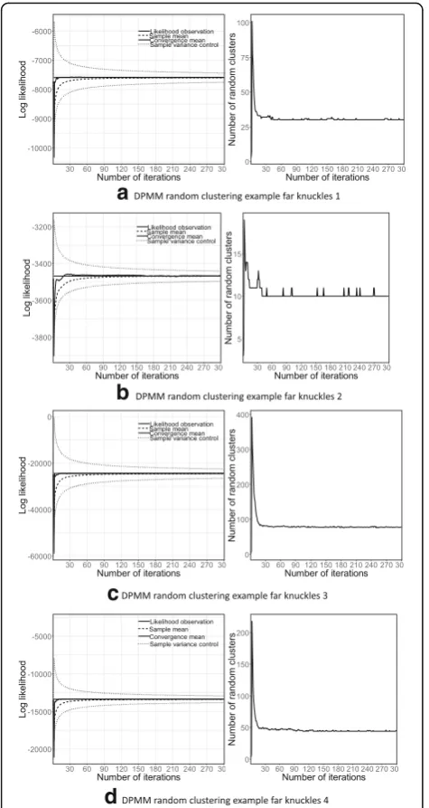
From the results, the convergence speed of DPMM is faster and the smoothness of the likelihood curve is greater. On the one hand, because the number of clus-ters is flexible, the model has further improved the identification of the structure within the training data-set. The process of testing the number of linked ran-dom clusters can further clarify the sampling results. In the initial phase of the iterative process, the number of clusters suddenly increases by several times the

convergence value. As shown in Figs.4 and5, different from the parameter optimization in the traditional fi-nite mixture model, this stage corresponds to the sam-pling algorithm performing a random search in a wide range of clustering models, so that the model can quickly determine a more stable clustering mode. On the other hand, the Dirichlet distribution uses an a priori structure, so that the update process of the DPMM internal parameters can be more effectively controlled under higher-level conditional distributions,

a

b

c

d

Fig. 4Convergence of DPMM random cluster of far knuckles.aDPMM random clustering example far knuckles 1.bDPMM random clustering example far knuckles 2.cDPMM random clustering example far knuckles 3.dDPMM random clustering example far knuckles 4

a

b

c

d

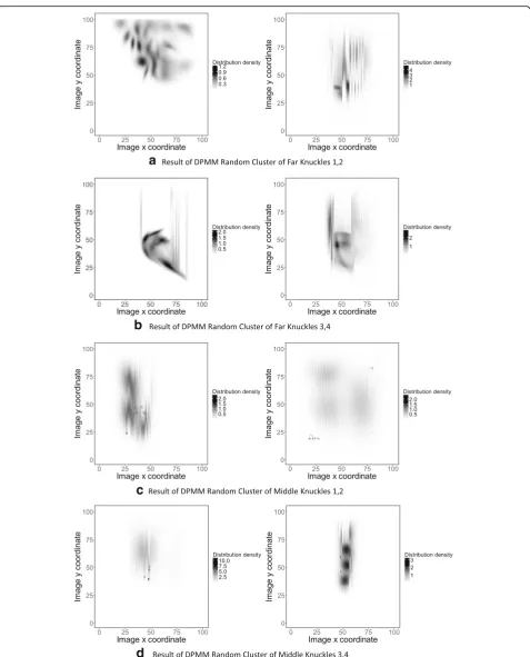
Fig. 5Convergence of DPMM random cluster of middle knuckles.a

a

b

c

d

manifesting that the convergence curve has higher smoothness in the stable region.

5.2 Offset measurement data learning results

Examples of the DPMM model learning results on the training image library are shown in Fig. 6. Under the condition of K= 3 clustering initialization, the flexible random clustering modeling for image high-offset dens-ity position distribution is realized. A high-level distribu-tion likelihood model of knuckle images with a more complex internal structure is obtained. The far phalanx goal learning results shown in the figure clearly show that the clustering self-adaptive process has similar re-sults to data density clustering. The model scale has a strong ability to adapt to the training set. The distribu-tion of clustering represented by the model likelihood results is not only consistent with the observed charac-teristics on the whole. The characteristic orientation of the internal clustering component also reflects the fea-tures of the knuckles under the grip of the hand. It shows that this algorithm has better modeling ability for the high-level distribution of far-knuckle images.

Using the aforementioned middle-level distribution learning and prediction algorithm, the multi-classification model of middle-level data for each image is learned in 51 positive images of distal phalanx images and 51 positive sample images of middle phalanx images, respectively, as

shown in Fig.7. In Fig.7, from left to right, there are first-, second-, and third-class hidden flags.

From the prediction results in Fig. 7, it can be seen that the three-category tag learning results of layer data in the finger image can more clearly show the design goals of the model. The marker results of the learning prediction also conform to the hypothesis of the distri-bution of layer data in the knuckle image.

Considering the learning accuracy and computational complexity of the fusion process, the lattice field [1 : 1 : 101]∗[1 : 1 : 101] generated after discretizing the feature plane is used as the discriminant field. We take the co-variance matrix as an isotropic exponential form:

k xð 1;x2Þ ¼ exp − x1−x2

k k2 κ

!

; ð68Þ

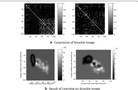
where the scale parameter is κ= 0.007. In the distal phalanx and middle-finger image test libraries (51 posi-tive and negaposi-tive samples), the high- and middle-level data-extraction process, feature likelihood calculation, and fusion model learning are completed. Based on the high-level data DPMM model learning results, the high-level data model likelihoods are obtained. We com-bine the mid-level three-classification model to calculate the likelihood value of the corresponding observation data and normalize the two similarity values as a labeled

a

b

test set for the supervised learning of the two-class Gaussian process. Multi-offset feature likelihood distri-butions, covariance functions, and fusion model (GP) learning results are shown in Fig. 8, in which the left graphs of each map are far-knuckle results, and the right graphs are the middle-finger results.

According to Fig.8b, in the normalized feature plane, the first characteristic direction of the positive sample fusion distribution follows the characteristic line (0, 0)-(100, 100) direction in the feature plane. The second feature direction is nearly perpendicular to the feature line; the first feature direction of the negative sample fu-sion distribution is close to the vertical direction of the feature line. The angle relationship between the feature direction and the feature line indicates that the two types of offset features that are fused constitute a certain degree of discrimination between positive and negative samples, and the fusion results show a stronger forecast of this differentiation. Comparing the left and right graphs shown in Fig. 8b, the high-end model of far-knuckle images has better discrimination between positive and negative samples than the middle-level model, while the fusion prediction of middle-finger im-ages shows the opposite result. The main reason for the difference between the above models is the obvious

differences in the random structure of the distal phalanx and middle phalanx images, which are embodied in the differences in distribution patterns at different levels of displacement.

5.3 Recognition for various algorithms

Under the fixed threshold condition, the recognition ability of the high-level data DPMM model, the middle-level data implicit marking GP model, and the DPMM+ GP model combining the two are briefly ana-lyzed. We artificially produced four finger-knuckle image databases with library capacity of 330, 1344, 1896, and 1400 images. These knuckles are taken by industrial cameras and come from people of different genders, ages and sizes. In these image libraries, positive and negative samples each make up half. In these image libraries, two are far-finger image libraries and two are middle-finger image libraries. To test the adaptability of the recogni-tion algorithm to the fuzzy objects, the joint features corresponding to all the knuckle images in the four image libraries are artificially selected to be weaker than those in the training library. That is, testing on a feature-rich joint image can achieve higher recognition capabilities. Three models are used in the four image li-braries for detection to compare the optimal recognition

a

b

ability of each algorithm for each image library; through the test analysis, the threshold of the highest recognition capability of the above three models in each image li-brary is taken as the best recognition threshold of each algorithm in the library and plotted to a receiver operat-ing characteristic curve (ROC). At the same time, through actual measurement, it is found that the differ-ence between the best recognition thresholds of the same algorithm in different image databases is small. Therefore, the following four ROC curves can be com-pared and analyzed as a whole, as shown in Fig.9.

Considering that the area under the curve (AUC) on the ROC is a measure of the recognition ability of the identifier, it can be clearly seen from Fig. 9 that in the far-knuckle test library, the comprehensive model recog-nition ability of the middle-level data model and the two-tier data is not as good as that of high-level image features. In the middle-finger test library, the recognition curves of the two high-level data models are low, and the corresponding AUC is less than 0.5. The recognition ability of the high-level data model in the far-finger li-brary is obviously higher, while the middle-tier data

model in the middle-finger library has stronger recogni-tion ability. The above shows that the existing data model has great differences in the ability to identify dif-ferent types of knuckle objects. It also potentially indi-cates that there is a certain difference between deep model categories in the distribution of far- and middle-finger image data.

In Fig.9b, the AUC values of the high-level data model corresponding to the two ROCs are 0.5134 and 0.2332. It can be seen that the recognition effect of high-level models in the middle-finger image database (2) is not obvious, and wrong classifications even appear. Further tests show that the high-level model with high likelihood is the middle-finger area, not the finger joint area. This phenomenon occurs because the intermediate region has relatively small local information entropy due to the smooth grayscale distribution. The high-level data vol-ume is larger and denser than the usual joint image data, which undermines the model’s assumptions on data dis-tribution, and therefore, it has poor recognition capabil-ity. At the same time, according to Fig.9, it can be seen that the ROC corresponding to the two-layer data fusion

a

b

model is located between the high- and middle-level models. It shows that the recognition based on the fu-sion model has the effect of comprehensively judging the two features. In the case that the high- and middle-level models differ greatly in their ability to iden-tify models, they can provide effective comprehensive evaluation, which is more prominent in Fig. 9b. The minimum area under the curve for the fusion model is (a) 0.4512 on the left of the figure, and the maximum is (b) 0.7880 on the right of the figure. The results show that the fixed threshold identification method has stable and correct classification ability under the condition of existing limited data and test set in the environment where the light intensity is relatively stable and the im-aging angle does not change much.

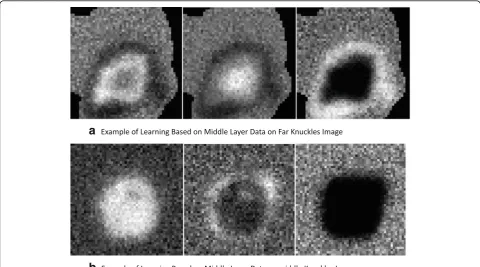
To further improve the recognition ability of the fusion model, combined with the learned DPMM+GP model, adaptive threshold joint detection is performed on a hand test image containing a finger joint. The size of the test image is controlled to include the size of about 1000 tem-plates, as shown in Fig. 10. Among them, black indicates that there is no finger joint at the position, the gray portion is the artificially marked finger joint region, and the white position is the joint point position result recognized by the adaptive threshold segmentation. When the detected joint position falls within the manually determined gray area, the joint identification is correct. Being away from the gray area indicates that the detected position has a large deviation

from the true position. With the aid of diffusion evolution, the recognition result is closer to the real target area, which obviously improves the accuracy of finger joint target rec-ognition. It is worth noting that the detection results and the marked areas shown in Fig.10are all at the pixel level. Therefore, the detection error of the above algorithm in the actual image is also at the pixel level. For actual detection tasks, joint detection can be initially implemented.

6 Conclusions

In this paper, nonparametric density kernel estima-tion results are used as observaestima-tion sets, and the es-timation of multi-level migration of knuckle images is estimated using both random clustering iterative learning and a multi-class random field model. Fur-ther, through the fusion learning of multilayer migra-tion features, the overall characteristics of knuckle images are constructed, and the detection and recog-nition capabilities of the above multiple models under fixed and adaptive thresholds are compared. At the same time, a knuckle position image recogni-tion algorithm based on an offset feature fusion model under adaptive threshold conditions is pre-sented. Threshold recognition is carried out on the image with relatively stable light intensity. The re-sults show that the corresponding algorithm is feas-ible. For the environment with large change of light intensity and the large change of camera angle, it is

a

b

necessary to further study the adaptability of image threshold.

Acknowledgements

The authors thank the editor and anonymous reviewers for their helpful comments and valuable suggestions. I would like to acknowledge all our team members, especially Luqi Gong. These authors contributed equally to this work.

About the authors

Shiqiang Yang was born in Baiyin, Gansu, P.R. China, in 1973. He received the Ph.D degree in mechanical engineering from Xi’an University of Technology of China, Xi_’an, China, in 2010. From 2005 to 2018, he was with Xi_’an University of Technology of China, Since 2009, he has been an associate professor with the School of Mechanical and Precision Instrument Engineering, Xi’an University of Technology, Xi’an, China. From 2011 to 2018, he conducted the Master Research with the School of Mechanical and Precision Instrument Engineering, Xi’an University of Technology, Xi’an. His current research interests include Intelligent robot control, Image recognition, behavior detection and recoginition.

Luqi Gong was born in Xianyang, Shaanxi, P.R. China, in 1991. He received the Master degree from the Xi’an University of Technology of China, Xi’an, China, in 2016. He research interests include image recognition, image processing and biometric detection.

Dan Qiao was born in Handan, Hebei, P.R. China, in 1994. He received the Bachelor degree from the Xi’an University of Technology of China, Xi’an, China, in 2016. Now, he works in Xi_’an University of Technology of China as Master student. He research interests include image recognition, image processing and biometric detection.

Funding

This work is supported by the National Natural Science Foundation of China (Grant No.51475365).

Availability of data and materials

Please contact author for data requests.

Authors’contributions

All authors take part in the discussion of the work described in this paper. These authors contributed equally to this work. All authors read and approved the final manuscript.

Competing interests

The authors declare that they have no competing interests.

Publisher’s Note

Springer Nature remains neutral with regard to jurisdictional claims in published maps and institutional affiliations.

Received: 24 September 2018 Accepted: 10 January 2019

References

1. Y. Wang, T. Chen, Z. He, C. Wu, Review on the machine vision measurement and control technology for intelligent manufacturing equipment. Control Theory Appl.32(3), 273–286 (2015)

2. M. Liu, J. Ma, M. Zhang, Z. Zhao, D. Yang, Q. Wang, Online operation method for assembly system of mechanical products based on machine vision. Comput. Integr. Manuf. Syst.21(9), 2343–2353 (2015)

3. Y. Wang, D. Ewert, R. Vossen, S. Jeschke, A visual servoing system for interactive human-robot object transfer. J. Autom. Control Eng3(4), 277– 283 (2015)

4. J.T.C. Tan, F. Duan, R. Kato, T. Arai, Safety strategy for human-robot collaboration: design and development in cellular manufacturing. Adv. Robot.24, 839–860 (2010)

5. M.K. Bhuyan, K.F. MacDorman, M.K. Kar, D.R. Neog, Hand pose recognition from monocular images by geometrical and texture analysis. J. Vis. Lang. Comput.28, 39–55 (2015)

6. D.-L. Lee, W.-S. You, Recognition of complex static hand gestures by using the wristband-based contour features. IET Image Process.12(1), 80_–87 (2018)

7. A. Moschetti, L. Fiorini, D. Esposito, P. Dario, F. Cavallo, Toward an unsupervised approach for daily gesture recognition in assisted living applications. IEEE Sensors J.17(24), 8395–8403 (2017)

8. P. Bao, A.I. Maqueda, C.R. del Blanco, N. García, Tiny hand gesture recognition without localization via a deep convolutional network. Consum. Electron.63(3), 251_–257 (2017)

9. A.V. Dehankar, S. Jain, V.M. Thakare,Using AEPI Method for Hand Gesture Recognition in Varying Background and Blurred Images, 2017 International conference of Electronics, Communication and Aerospace Technology (ICECA), vol 1 (2017), pp. 404_–409

10. Y. Ding, Q. Zhao, B. Li, X. Yuan, Facial expression recognition from image sequence based on LBP and Taylor expansion. IEEE Access5, 19409–19419 (2017)

11. C. Yao, Y.-F. Liu, B. Jiang, J. Han, J. Han, LLE score: A new filter-based unsupervised feature selection method based on nonlinear manifold embedding and its application to image recognition. IEEE Trans. Image Process.26(11), 5257–5269 (2017)

12. J. Wang, G. Wang, Hierarchical spatial sum_–product networks for action recognition in still images. IEEE Trans. Circuits Syst. Video Technol.28(1), 90– 100 (2018)

13. P. Panda, A. Ankit, P. Wijesinghe, K. Roy, FALCON: feature driven selective classification for energy-efficient image recognition. IEEE Trans. Comput. Aided Des. Integr. Circuits Syst.36(12), 2017–2029 (2017)

14. H. Li, A. Achim, D. Bull, Unsupervised video anomaly detection using feature clustering. IET Signal Process.6(5), 521–533 (2012)

15. J.-Y. Jiang, R.-J. Liou, S.-J. Lee, A fuzzy self-constructing feature clustering algorithm for text classification. IEEE Trans. Knowl. Data Eng.23(3), 335–349 (2011)

16. M. Rahmani, G. Akbarizadeh, Unsupervised feature learning based on sparse coding and spectral clustering for segmentation of synthetic aperture radar images. IET Comput. Vis.9(5), 629–638 (2015)

17. R.B. Dan, P.S. Mohod, Survey on Hand Gesture Recognition Approaches [J]. Int. J. Comput. Sci. Inf. Technol.5(2), 2050–2052 (2014)

18. P. Garg, N. Aggarwal, S. Sofat, Visual based hand gesture recognition. Int. J. Comput. Electr. Autom. Control Inform. Eng.3(1), 186–191 (2009) 19. Fai CC, Silvia A, Alessandro B, Alain F, Mehdi M, Francesco, P. Constraint

study for a hand exoskeleton: human hand kinematics and dynamics. J Robotics. 2013:1-17.https://doi.org/10.1155/2013/910961.

20. S. Kang, B. Choi, D. Jo, Faces detection method based on skin color modeling. J. Syst. Archit.64(C), 100–109 (2016)

21. G. Wu, W. Kang, Robust fingertip detection in a complex environment. IEEE Trans. Multimedia18(6), 978_–987 (2016)

22. A. Kumar, C. Ravikanth, Personal authentication using finger knuckle surface. IEEE Trans. Inf. Forensics Secur.4(1), 98–110 (2009)

23. K. Usha, M. Ezhilarasan. Hybrid Detection of Convex Curves for Biometric Authentication Using Tangents and Secants. The 3rd IEEE International Advanced Computer Conference, Ghaziabad, India, February 22–23, 2013: 763–768. Adv. Comput. Conf., 2013 , 7903 (5) :763–768

24. K. Usha, M. Ezhilarasan, Finger knuckle biometrics–a review. Comput. Electr. Eng.45(C), 249_–259 (2014)

25. H.-C. Huanga, C.-T. Hsiehb, M.-N. Hsiao b, C.-H. Yehb, A study of automatic separation and recognition for overlapped fingerprints. Appl. Soft Comput.

71, 127–140 (2018)

26. K. Usha, M. Ezhilarasan, Fusion of geometric and texture features for finger knuckle surface recognition. Alex. Eng. J.55(1), 683–697 (2016)

27. K. Usha, M. Ezhilarasan, Robust personal authentication using finger knuckle geometric and texture features. Ain Shams Eng. J. (2016) In press 28. Z. Lin, L. Zhang, D. Zhang, H. Zhu, Online finger-knuckle-print verification for

personal authentication. Pattern Recogn.43, 2560–2571 (2010)

29. G. Gao, L. Zhang, J. Yang, L. Zhang, D. Zhang, Reconstruction based finger-knuckle-print verification with score level adaptive binary fusion. IEEE Trans. Image Process.22(12), 5050_–5062 (2013)

30. A. Kumar, Z. Xu, Personal identification using minor knuckle patterns from palm dorsal surface. IEEE Trans. Inf. Forensics Secur.11(10), 2338–2348 (2016)

31. S. Yang, L. Gong, Excursion characteristic learning and recognition for hand image knuckles based on log Gaussian Cox field. Trans. Chin. Soc. Agric. Machinery48(1), 353–360 (2017)