R E S E A R C H
Open Access
Efficient evaluation of the Number of
False Alarm criterion
Sylvie Le Hégarat-Mascle
*, Emanuel Aldea and Jennifer Vandoni
Abstract
This paper proposes a method for computing efficiently the significance of a parametric pattern inside a binary image. On the one hand, a-contrario strategies avoid the user involvement for tuning detection thresholds and allow one to account fairly for different pattern sizes. On the other hand, a-contrario criteria become intractable when the pattern complexity in terms of parametrization increases. In this work, we introduce a strategy which relies on the use of a cumulative space of reduced dimensionality, derived from the coupling of a classic (Hough) cumulative space with an integral histogram trick. This space allows us to store partial computations which are required by the a-contrario criterion and to evaluate the significance with a lower computational cost than by following a straightforward approach. The method is illustrated on synthetic examples on patterns with various parametrizations up to five dimensions. In order to demonstrate how to apply this generic concept in a real scenario, we consider a difficult crack detection task in still images, which has been addressed in the literature with various local and global detection strategies. We model cracks as bounded segments, detected by the proposed a-contrario criterion, which allow us to introduce additional spatial constraints based on their relative alignment. On this application, the proposed strategy yields state-of the-art results and underlines its potential for handling complex pattern detection tasks.
Keywords: Image analysis, Number of False Alarms, cumulative space, A-contrario decision, Crack detection
1 Introduction
Since the seminal articles of Desolneux et al. [1,2], detec-tion approaches based on the Number of False Alarms (NFA) criterion became more and more popular in the field of image processing over the last decade. In these approaches, the words “a-contrario” refer to the fact that detection is performed by contradicting a “naive” model that represents the statistics of the outliers (the null hypothesis in statistical decision theory). Then, the inliers are detected as too regular to appear “by chance” accord-ing to the naive model. The main asset of such approaches is their independence from threshold parameters, since they cast the detection as an optimization problem by maximizing thesignificancedefined from deviation rela-tively to the naive model. Then, to interpret this maximum of significance (or, equivalently, minimum NFA value) in terms of the presence or absence of structured pattern, one refers to the NFA definition itself: the NFA of a
*Correspondence:[email protected]
SATIE Laboratory, Université Paris Sud, rue Noetzlin, Orsay, France
pattern candidate is the expected number of false pos-itives (random patterns) occurring in the search space when accepting all patterns at least as significant as the candidate. By setting the NFA detection threshold to 1 irrespective of the detection task, the a-contrario frame-work simply states that the upper bound for detecting a random rare event is at most one occurrence.
After the introductory illustration of a-contrario meth-ods on alignment detection [1] grounded in the Gestalt continuity principle, a number of works has developed around the idea of using this fundamental pattern in order to detect derived structures such as segments [3–5], vanishing points [6,7], or scratches [8], while recent works [9,10] show the ongoing interest about detection of basic alignments. Nevertheless, a-contrario methods have simultaneously evolved to deal with the detection of more complex patterns, such as circles and ellipses [11,12] as well as coherent clusterings in a broader sense [13–18].
Considering pattern recognition problems, in order to find the most significant subset among the ones represent-ing patterns, one should theoretically compute the signifi-cance of every possible pattern. If the researched patterns
correspond to parametric objects (e.g., lines, ellipses), the dimension (and thus the actual cardinality being used) of the solution space to explore grows with the num-ber of parameters. Then, in order to maintain tractability, discretizing the parameter space or relying on heuris-tics [4] for exploration are commonly employed strate-gies. In this work, we show how a cumulative space may be used in order to compute efficiently the significance of a given parametric pattern. Cumulative approaches, widely used in pattern recognition and introduced in [19], rely on a quantization of the entire feasible parameter space denoted as accumulator, in which every observation increments the count of every discrete cell (i.e., pattern) consistent with the existence of that observation. At the end of the process, each cell records the total number of supporting observations.
In our work, we show that in some favorable cases there is an equivalence between considering cells in a high-dimensionality cumulative space and recasting them as n-orthotopes in an alternative cumulative space of decreased dimensionality (by 1 or 2 in the proposed examples). Now, using a trick similar to the integral his-togram [20], the fact of considering n-orthotopes allows for an efficient computation of the required NFA val-ues. Specifically, the integral histogram is the result of the propagation of an aggregated histogram from ori-gin through the whole image lattice. In this way, the histogram of any rectangular region may be computed by simple arithmetic operations between four points of the integral histogram. By leveraging the use of this cumulative space of reduced dimensionality, we are thus able to lower significantly the complexity of pat-tern research and to extend the limits of the param-eter space dimension due to the available computer memory size.
Then, as a second contribution, we show how crack detection in still images can benefit from the proposed coupling between an a-contrario criterion and a cumula-tive space.
2 Methods
2.1 Related work
In previous works involving NFA criterion, two “naive” models have been widely used, namely the Gaussian and Bernoulli models that stand for gray level and binary images, respectively. In this study, we focus on the second case. Pixels take then values in {0, 1} set (or
false,true set). Assuming a Bernoulli distribution of parameter p for pixel binary values, the probability to
have a given number κ of truesamples, called 1-valued
pixels in the following of the paper, among a given number ν of pixels is a Binomial distribution of param-eter p. Then, according to [21], the Number of False Alarms is
NFAB(κ,ν,p)=η2
ν
i=κ
ν i
pi(1−p)ν−i, (1)
whereη2is the “number of tests” coefficient that depends
on the number of possible patterns ofνpixels.
The significance value, being defined as S(κ,ν,p) = −ln(NFAB(κ,ν,p)), may be derived from Eq. (1). Using the Hoeffding’s approximation like in [22], we may express S(κ,ν,p) in terms of the Kullback-Leibler divergence (K-L) between the 1-valued pixel probability restricted to a particular area,pa= κν, and the naive model probability p:∀(κ,ν)such thatκν >p,
S(κ,ν,p)≈ν
κ νln
κ/ν
p
+1−κ ν ln
1−κ/ν
1−p
−lnη2
(2)
2.2 Proposed approach: NFA computation using a cumulative space
According to Eqs. (1) or (2), in order to compute the signif-icance of a given pattern, we need both its geometric area or its number of pixels and its number of 1-valued pixels.
The main idea of this work is to use a cumulative space to store partial sums of numbers of points in order to decrease the computational cost. Then, the number of points in any pattern of given parameters can be directly retrieved from the values stored in the cumulative space, allowing us to accelerate the algorithm and/or to cope with a finer discretization of the parameter space.
In the following part of this section, we explain our approach and we illustrate how it works through four clas-sic examples, namely detection of rectangular tiles, strips, rings and bounded strips.
2.2.1 Use of cumulative space
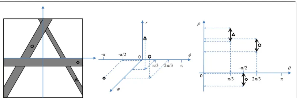
allows us to use the same 2D cumulative space as that of straight lines, namely the classic Hough transform space.
Figure 1 illustrates the possible representations for a strip, in particular as a point in a 3D space involving polar coordinate parameters(φ,r) ∈ [−π,+π]×R+ or as a line segment in a 2D space involving polar coordinate parameters(θ,ρ)∈[0,+π]×R. In this latter case, theρ parameter variation (along the line segment,ρ∈[ρ0,ρ1])
simultaneously codes the two parameters(r,w)of 3D rep-resentation so that to find the points voting for a strip, we can simply sum the votes between(θ,ρ0)and(θ,ρ1).
According to this last representation, the “strip” pattern (with 3 parameters) can be processed as a set of “straight lines” that are simpler patterns (having only 2 parameters). Therefore, among several parametric forms of a given pattern, denotedb, we favor the one that is a set of simpler patterns, denoteda, potentially having several parameters that can be represented on a same axis of the cumu-lative space. Such a representation allows us to reduce the dimensionality of the cumulative space and save pro-cessing time by storing partial sums, in a similar fashion to integral histograms [20]. Specifically, it allows us to compute the pattern as follows.
Let l denote the number of parameters required to
determine the considered patternb. We denote byβ =
(βi)i∈[1,l]the tuple of these parameters which take values
inA(Adepends on the image lattice and on the applica-tion that may introduce some specific constraints on the parameters).
LetCbe the considered cumulative space. If patternb has been parametrized as a set of “well-chosen” patterns a,Cis the cumulative space associated toa parametriza-tion ofa. Sinceahas less parameters thanb, some pairs ofbparameters are bounds for intervals ofaparameters.
Then, we distinguish in C the axes that represent only
one parameterβi and the axes that represent two differ-entβi(playing the role of bounds for someaparameters). For example, in Fig.1,Cis the polar representation space, denoted by the two parameters(θ,ρ), with one axis that represents the angleθ, and the other axis that represents the two bounds forρ parameter. Since this last axis car-ries in fact two parameters, it is calledbi-parameteraxis, in opposition to an axis that carries only one parameter such asθ-axis in this example. Ifmis the number of
bi-parameter axes, with 0 ≤ m ≤ 2l, C dimensionality is
l−m, andl−2mis the number of mono-parameter axes. Note that inC, a simpler pattern is represented by a point and a pattern of interest by a n-orthotope (also called hyperrectangle). Indeed, any pattern of interestbis then represented by a n-orthotope ofChavingl−2m dimen-sions reduced to a single point and the other dimendimen-sions which are non-null intervals. Now, sinceC is a cumula-tive space associated to patterna, the number of votes for a given patterna is provided by the value of the corre-sponding point inC, and the number of votes for a given pattern b is the sum of the point values in C over the corresponding hypercube.
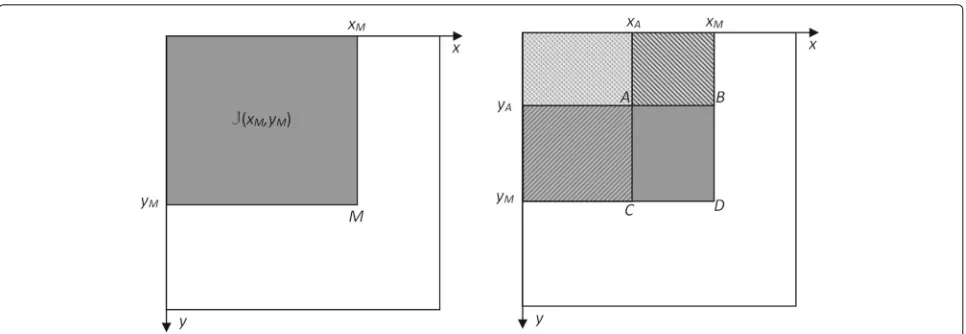
Finally, following the integral histogram idea [20], we have to compute and store partial sums overC. Figure2 illustrates how integral histogram allows us to compute any sum or integral on a rectangular domain from the storage of the partial sums (integrals) from the origin to any pointM, i.e., in 2D case as illustrated in the figure, from(0, 0)toM(xM,yM). To be able to specify the partial sum computation, we have to order the parameters.
Without loss of generality, the elements of β tuple
are mapped to the C axes, denoted (αi)i∈[1,l−m], as
fol-lows: the l − 2m first components are mapped to the
l − 2m first C parameter axes (that are thus
mono-parameter axes) and the 2mlast components are mapped
Fig. 1Possible representations of strips. Case of three strips represented as follows: pixel sets in the image domain (left), points in the 3D parameter space corresponding to polar line representation enriched with width parameter (middle), and line segment in the 2D parameter space
Fig. 2Illustration of the Integral Histogram trick. Case of two bi-parameter axes,xandy; left: visualisation on the 2D integration or summation domain associated toJ(M)value; right: illustration of the computation of the integral (sum) on any rectangular domain ABDC by finite difference betweenJvalues at its four corners:J(D)−J(C)−J(B)+J(A)
to the m last C parameter axes (that are thus
bi-parameter axes) so that theβi parameters are reordered
as
(αi)i∈[1,l−2m],
αj j∈[l−2m+1,l−m],
αj
j∈[l−2m+1,l−m]
,
whereαjdenotes an interval lower bound andαjdenotes an interval upper bound.
In the following, for conciseness and since we focus on bi-parameter axes, the list of parameters of mono-parameter axes (that may possibly be empty) is denoted bydots. Then, ifJC denotes the cumulative space instance where the value of a point represents its number of votes and if we choose a unit step for the cumulative space res-olution, the cumulative space instance containing partial sumsJCis computed as follows: ifm=1,
JC. . .,αl−1
=JC. . .,αl−1
+1[αl−1>1]JC. . .,αl−1−1
, (3)
where1[αi>1]denotes the indicator function that takes the
value 1 if the condition between square brackets is true and value 0 if otherwise; and ifm=2,
JC. . .,αl−3,αl−2
=JC. . .,αl−3,αl−2
−1αl−3>1 αl−2>1
JC. . .,αl−
3−1,αl−2−1
+1 αl−3>1
JC. . .,αl−3−1,αl−2
+1 αl−2>1
JC. . .,αl−3,αl−2−1
.
(4)
FromJC, the number of 1-valued pixels in a given pat-tern such that(αi,i∈[1,l−2m]) = b1(possibly
nonex-istent if l = 2m) and ∀i ∈ [l−2m+1,l−m], αi ∈
αi,αi
is:
• ifm=1,
κ (b)=
αl−1
αl−1=αl−1
JCb1,αl−1 =JC
b1,αl−1 −JC
b1,αl−1 ,
(5)
• ifm=2,
κ (b)=
αl−3
αl−3=αl−3
αl−2
αl−2=αl−2 JC
b1,αl−3,αl−2 ,
=JCb1,αl−3,αl−2 +JC
b1,αl−3−1,αl−2−1
−JCb1,αl−3−1,αl−2 −JC
b1,αl−3,αl−2−1 .
(6)
In summary, the main idea of the paper is that the NFA can be computed more efficiently with
cumula-tive space pre-computation: for an image of size N2,
using the integral histogram trick in a well-chosen cumu-lative space of reduced dimension l−m (instead of l)
with each single dimension of size M, the complexity
is roughlyN2 (JC computation) +Mm (JC computation)
+Ml. Then, reducing the complexity compared to a com-plete brute force approach in N2×Ml allows for more precise results by providing finer estimation of pattern parameters.
Let us now consider four classic examples, namely rectangular tiles, strips, rings, and bounded strips, by specifying for each case the corresponding cumulative space. These patterns are detected on an image having Nccolumns andNr rows and half diagonal lengthρd =
1 2
N2
• Rectangular tiles are parametrized as sets of 2D points, using the coordinates of two opposite corners: (xUL,yUL,xLR,yLR)wherexULandyUL(respectively xLRandyLR) denote the image coordinates (column and row) of the upper left (respectively lower right) corner of the tile;xUL∈[1,Nc],yUL∈[1,Nr], xLR∈[xUL,Nc]andyLR∈
yUL,Nr
. The cumulative spaceT has two dimensions: the column axisx representingxULandxLRand the row axisy
representingyULandyLR.JT is the binary image itself
andJT, the cumulative space containing the partial sums ofJT, is derived from Eq. (4) withl=4,m=2, αl−3=xandαl−2=y.
• Strips are parametrized as sets of parallel straight lines, through the polar coordinates of the two border lines:(θ,ρ0)and(θ,ρ1), whereθis the parallel line
direction (one single value) andρ0andρ1the
distances of the border lines to the space origin. Choosing the image center as origin,ρ0andρ1are
signed values so that there is no discontinuity inρ values for strips containing the origin. Then, θ ∈[0,π),ρ0∈[−ρd,ρd],ρ1∈[ρ0,ρd]. The cumulative spaceShas two dimensions: the angular axisθand the distance axisρrepresentingρ0andρ1.
JSis the classic Hough transform [19], andJSis the cumulative space containing the partial sums ofJS, derived from Eq. (4) withl=3,m=1andαl−1=ρ. • Rings are parametrized as sets of concentric circles,
through the circle center coordinates(x0,y0)and two
raysρ0andρ1respectively, wherex0∈[1,Nc],
y0∈[1,Nr],ρ0∈[0,ρd],ρ0∈[ρ0,ρd]. The
considered cumulative spaceRhas three dimensions: the column and row axesx and y for the coordinates of the center, and the ray axisρrepresentingρ0and
ρ1.JRis the circle Hough transform, andJRis the
cumulative space containing the partial sums ofJR, derived from Eq. (4) withl=4,m=1andαl−1=ρ. • Bounded strips are sets of parallel segment lines that
can also be represented as unbounded strips with two extremities. They are parametrized by a 5-tuple (θ,ρ0,φ,ρ1,ψ)where(θ,ρ0,ρ1)represents the
unbounded strip as previously stated, andφ,ψare the angular coordinates of the extremities:θ ∈[0,π), (φ,ψ)∈[0, 2π)2,ρ0∈[−ρd,ρd],ρ1∈[ρ0,ρd]. The considered cumulative spaceBhas three dimensions, namely the strip angle axisθ, the distance axisρ representingρ0andρ1, and the extremity angular
coordinate axisφrepresentingφandψ.JBis the half-line Hough transform (e.g., a 1-valued pixel votes only for the line segments containing it having the starting point with the lower angular coordinate), and
JBis the cumulative space containing the partial
sums ofJB, derived from Eq. (4) withl=5,m=2, αl−3=ρandαl−2=φ.
2.2.2 Algorithm
Algorithm 1 describes the way the most significant pat-terns are detected using the NFA criterion coupled with cumulative spaces. Its inputs are as follows: the considered binaryimageI, the cumulative spaceCdetermined by the considered pattern (for conciseness,Cbi-parameter axes are denoted as “bip-axes”), and the set of possible patterns
A, which is determined by image dimensions and
possi-bly by some application-specific constraints. The output of Algorithm 1 is the collection of the most significant pat-terns,P. Note that here we use the termcollectionto avoid a possible confusion with the termset, which we already use to refer to a group of simpler patterns. After the initial-ization step, the algorithm begins a loop that successively detects the patterns that will be added, one by one, toP as the most significant pattern at the current iteration. At each iteration,JC is computed according to Eq. (3) or to Eq. (4) depending on the value ofm(in this work, we focus onm∈ {1, 2}but the generalization is trivial). Then, two vectorsκ[ .] andα[ .] of dimensionalityN, the number of pixels assumed to be the maximum size of a pattern, are allocated. Note thatκ[.] elements are integer values and
α[.] elements arel-tuples. They will store, for each pat-tern sizejin pixel unit, the maximum number of 1-valued pixels (inκ[j]) and the corresponding pattern parameter tuple (inα[j]). Indeed, for a given pattern area, the signifi-cance increases with the number of 1-valued pixels within it. Then, it is not necessary to compute the significance values for each pattern, but only for the patterns hav-ing different areas (in pixels) and achievhav-ing the maximum number of 1-valued pixelsκ[j]. For this reason, the signif-icance computation is done only after having selected, for each different size of pattern, the pattern having the high-est number of 1-valued pixels: the first loop selects these patterns; then, a second loop computes their associated significance value while at the same time searching for the maximum one, which is stored inSmaxalong with the cor-responding pattern stored inb. Finally, having found the most significant patternαˆ at the current iteration, we add it to the collection of significant patternsP only if the global significance of the collection of patterns increases. If it is not the case, the algorithm ends. Otherwise, before reiteration, the located pattern is removed from the image. In our case, when we remove a pattern, we do not set to falseall its pixels, but only the exceeding ones relative to naive model parameter p. Practically, for each 1-valued pixel located in the area of a primary pattern, we draw ran-domly its new value (0 or 1) according to the probability p. Although sub-optimal, this simple adjustment allows us to avoid penalizing too much patterns which overlap other patterns previously detected.
Algorithm 1:Detection of the most significant pat-terns
Data: Binary data imageI, cumulative spaceChaving mbip-axes, set of possible patternsA;
Result: Set of most significant patternsP; 1 N←number of pixels inI;
p← number of 1-valued pixels inN I;
2 Initialize setPto∅and real numberSP to 0; 3 Initialize booleanfinishedtofalse;
4 do
5 InitializeJCwith the transform ofIinC;
6 ModifyJC by computing the partial sums along
bip-axes;
7 Initialize vectorsκ[.],α[.] of dimensionalityNto 0;
8 forevery l-tupleα=(α1,. . .,αl)ofAdo
9 b←pattern of parametersα;
10 ν←area (in pixels) ofbpattern;
11 κ (b)←number of 1-valued pixels inb
deduced from points
12 ofJC(according to Eq. (5) ifm=1 or Eq. (6) ifm=2);
13 ifκ (b) >κ[ν]then
14 κ[ν]←κ (b);α[ν]←α; 15 end if
16 end for
17 InitializeSmaxandbto 0; 18 forν∈[1,N]do
19 if κ[νν]>pthen
20 S←S(κ[ν] ,ν,p)computed according
to Eq. (2);
21 ifS>Smaxthen
22 Smax←S;
23 b←pattern of parametersα[ν];
24 end if
25 end if
26 end for
27 S∪←significance ofP∪ {b}computed
according to Eq. (2); 28 ifS∪>SPthen
29 P ←P∪ {b};SP ←S∪; Remove patternb
fromI;
30 else
31 finished←true 32 end if
33 whilenot finished;
adapted. For instance, let us consider the case of φ ∈
π
2,34π
andψ ∈ 74π, 2π, since theoretically(φ,ψ) ∈ [ 0, 2π)2, an intermediate bound noted by its angle ϕ is such thatϕ∈[ 0,φ)∪(ψ, 2π); to haveϕ∈(φ,ψ)or(ψ,φ),
in this case, we change ψ ∈ −π4, 0. In a more
gen-eral case, to get the intermediate bound between φ and
ψ, we consider as new bound the pre-image of the image ofψ closest toφ(thus enforcing the monotonicity of the projection).
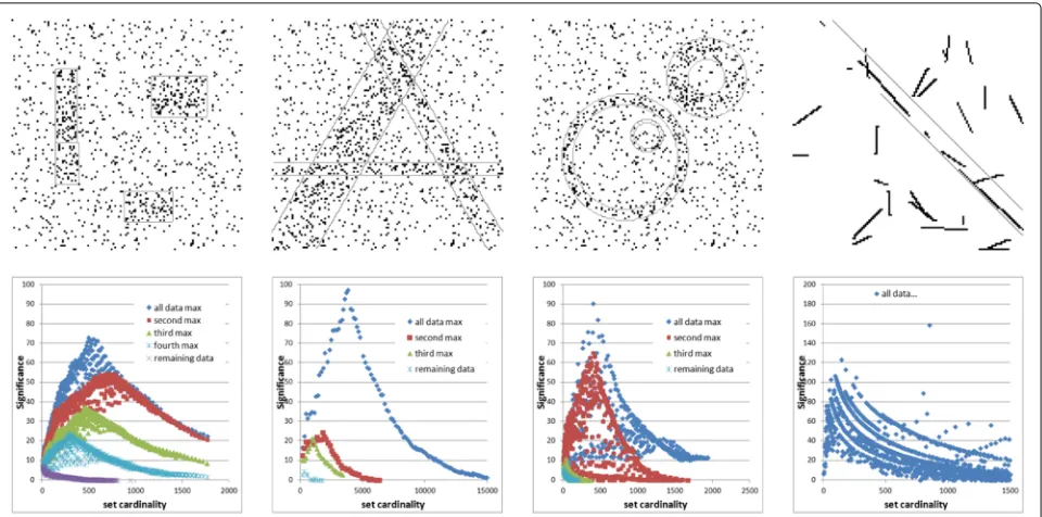
Figure3illustrates the detection of the parametric pat-terns introduced in the section. For each case (tile, strip, ring and bounded strip), the first row shows the simu-lated binary image (1-valued pixels in black and 0-valued ones in white) on which the detected pattern frontiers are superimposed in thin light gray. The second row shows the highest significance values versus the cardinality of the considered pattern (ν parameter in Eqs. (1) and (2) and in Algorithm 1). In these figures, each point repre-sents the highest significance value achieved by setting the cardinality value ν and varying the pattern parame-ters. It means that, given the type of pattern (tile, etc.) and the considered binary image, among all the patterns hav-ing the same number of pixels (νvalue on x-axis value),
the significance achieves its maximum value at the y
-value of the point. In the first three examples, there are three patterns to detect and only one in the last exam-ple (bounded strips). The different colors correspond to the different iterations showing the effect of removing a detected pattern from the image. In other words, they show the highest significance points obtained consider-ing either the whole initial set of 1-valued pixels (pre-sented on first row) or 1-valued pixel subsets derived by removal of the points belonging to the patterns already detected. Note that in the case of the tile, one of the the patterns is detected in two parts. However, we observe the very good robustness of the proposed detection process.
The complexity calculation presented in the previous section allows us to derive the algorithm complexity in terms of the polynomial order, but for the sake of brevity, it does not evaluate the leading constants and introduces simplifications on the cumulative space dimen-sions (assumed to be all the same). Thus, in order to provide some experimental values supporting the bene-fit of our proposal, Table1 shows the average execution times in the case of the toy example images (of size 128 × 128 pixels) in which three objects (either tiles, strips, or rings) have to be detected. The naive imple-mentation refers to a version that simply computes the number of 1-valued pixels for every possible instance of the considered pattern by scanning the binary image. Note that the computation of the corresponding areas (also needed) is straightforward since a geometric for-mula can be applied. From Table1, the time gain factor varies between about 103and 4×10³depending on the considered pattern and on the considered intervals for its parameters.
Fig. 3Toy example. Examples of parametrized objects’ detection using cumulative space to compute significance criterion. First row: simulated binary image of 1-valued pixels, representing the generic input. Second row: the highest significance values versus the cardinality of the considered pattern
3 Crack detection in still images
The proposed approach is suited for applications involv-ing a significance measure or NFA criterion, and ben-efiting from a finer sampling of the pattern space. For detection tasks that are quite standard a-contrario prob-lems, the basic idea is that the detection relies on pat-tern significance (or NFA) that itself depends on the number of 1-valued pixels belonging to the considered pattern. For instance, for detection estimated at region-level, i.e., in rectangular windows, the refinement of the space would imply the sampling to be performed with a 1-pixel sliding step in both dimensions, rather than using a non-overlapping or half-overlapping window sampling strategy [21]. Undoubtedly, the benefit of the proposed method will be more important for patterns with a high number of parameters, i.e., involving high dimensionality of the parametric space.
Table 1Comparison of running times (in seconds) of the proposed approach based on use of cumulative space and a naive implementation; case of the toy example patterns involving three objects to detect in each simulated image; running times averaged on 5 realisations on a standard laptop computer (Core i7 [email protected], 4Go RAM)
Pattern Proposed use of cumulative space
Naive
implementation
Time gain factor
Tiles 0.842 s 521.4 s 619
Strips 1.622 s 6095 s 3757
Rings 3.622 s 4501 s 1243
In this study, we have chosen to illustrate our refinement algorithm on the problem of crack detection.
Crack detection has indeed critical importance for ensuring the security of infrastructures and for minimiz-ing maintenance costs. In terms of appearance, a crack is a discontinuity in the background with respect to the under-lying material (e.g., asphalt for roads or concrete for walls). Then, it may be detected based on some photometric and geometric features [23] that are exploited by several pro-posed approaches (e.g., [24, 25]) which perform rather well on cracks observed on smooth and homogeneous surfaces (e.g., concrete).
However, these methods often fail when the background exhibits a noisy texture like in the case of road pavement.
radiometric features alone do not allow us to distin-guish the cracks from the road background and the geometric features should be also considered like in [27]. However, whereas [27] focuses on the modeling of the spatial interactions between line segments, in this work, we focus on the detection of these line segments based on significance (or NFA) computation. The back-ground heterogeneity due to asphalt textons resembles indeed well the null hypothesis. On such a background, the lines that compose the cracks may be seen as a deviation from the naive model, thus having high values of significance.
3.1 Related work
Crack detection approaches generally involve a prepro-cessing step that aims at computing a new data image on which the detection will be easier. The preprocessing step may consist in removing adverse or clutter features (e.g., shadow removal [26]), or in enhancing the pattern, e.g., by subtracting the median filtered image [25], or in stressing the filiform feature of the cracks e.g. by using Laplacian of Gaussian or steerable filters [28,29]. In this work, we consider the same preprocessing step as in [30]. Basically, it involves the shadow removal by background subtrac-tion and the estimasubtrac-tion of a new radiometric image, whose values gather both gray level information and gradient orientation features.
Then, from the preprocessed image, two analysis scales may be considered for crack detection itself. In [24,31], the detection is based on a local analysis performed across the whole image space using a sliding window, whereas in [26,32,33] the detection relies on a global process related to the expected photometric properties of cracks, based on the computation of minimum cost paths. The local or global search strategy and the parameters required by the algorithms set the scale for the patterns to be detected. Now, we observed that the cracks may be highly vari-able in terms of scale, thinness, and relative contrast. Thus, both local and global scales seem relevant and will then be considered in the proposed approach, through the measure of significance relatively to the context in a multi-scale reasoning.
Finally, note that since the used NFA criterion applies to binary images, we perform an automatic thresholding operation on the pre-processed image to derive theseed image, i.e., the binary image where 1-valued pixels are very likely to belong to the crack. Then, the objective of the whole algorithm presented in next section is to remove the false positives and to correct the false negatives on this seedimage.
3.2 Crack detection algorithm
Following a multi-scale strategy, we adopt a two-step algo-rithm. The input image is the binary image of the seeds
in which the 1-valued pixels represent (in an incomplete way and including some false positives) the researched patterns. The first step deals with local scale, and aims at determining the most significant local alignments of 1-valued pixels, that are calledelementary stripsin the fol-lowing. Then, the second step is intended to identify the significant straight chains of elementary strips.
Algorithm 2 describes the method based on the two successive steps. In Algorithm 2, a window refers to the rectangular image sub-area used for local detec-tion. Its dimensions in columns and rows are given as input parameters. Then, in every considered window, the elementary strips are detected as the most significant unbounded strip(s), following Section2.2. At the end of this step, a new binary image is derived such that the 1-valued pixels are exclusively located in detected sig-nificant local strips. In other words, the maximization of significance at local scale (over each window) is used as a filtering process which removes a part of the false
Algorithm 2:Crack estimation;Iis the image of the
seeds, operator∧ between two binary images is the
binary AND operator applied at pixel level Data: Binary image:I; window size;
Result: Binary imageISof cracks approximated by window strips;
1 Nc←number ofIcolumns;Nr←number ofIrows; 2 I←binary image of sizeNc×Nrinitialized with
falsevalues;
3 Set of possible extremities for bounded strips:E← ∅; 4 forevery non-overlapping window W of Ido
5 IW←the restriction ofItoW;
6 SW ←output of Algorithm 1 having inputs:IW,
Hough space having 1 bip axis andAthe set of any strip inIW;
7 forevery strip skofSWdo
8 Compute its restrictionsW,ktoWinI;
9 Set the pixels ofsW,kto valuetrueinI;
10 Add extremities ofsW,ktoE;
11 end for
12 end for
13 SI ←output of Algorithm 1 having inputs:I∧I, cumulative space for bounded strips having 2 bip axes andAthe set of bounded strips having extremities inE;
14 IS←binary image of sizeNc×Nrinitialized with
falsevalues;
15 forevery bounded strip bkofSI do 16 Set the pixels ofbkto valuetrueinIS; 17 end for
positives present in the seed image. Besides, the extrem-ities of local strips are also stored as possible extremextrem-ities of the bounded strips which are estimated in the next step. Then, at image scale, the most significant bounded strip(s) are detected following Section 2.2. Finally, the cracks are approximated by the concatenation of the ele-mentary strips (detected at local scale) that also belong to a bounded strip detected at image scale.
4 Results and discussion
We have applied the proposed algorithm to the public CrackTree dataset provided by [26], which illustrates our approach very well since noisy texture and other degra-dation artifacts are commonly present on the asphalt surface.
Algorithm 2 inputs are the binary image of the seeds and the window size used for local analysis. In CrackTree dataset, the image size is 800×600 pixels. In Section4.1, we choose to divide each image dimension by 10, so that the resulting window size is 80×60. In Section4.2, we val-idate more accurately this parameter’s choice. Regarding the seed image, we use the same preprocessing step as in [30]. Specifically, we use Algorithm 1 of [30] that includes a final thresholding operation with respect to an auto-matically derived threshold according to a NFA criterion operating at grayscale pixel level. However, this algorithm takes in input a standard deviation parameter that can be either automatically estimated from the grayscale image, or carefully chosen. This allows us to modulate the auto-matic threshold estimation. In Section 4.1, we consider the default value for this standard deviation, whereas in
Section 4.2 we also consider results obtained with an
alternative value to test the robustness of our results. To evaluate quantitatively the obtained results, the pre-cision and recall parameters are computed while distin-guishing between the mis-detection and the mis-location of a crack as follows. As in [27], the true positives and the false positives are computed by comparing the detec-tion results with incrementally dilated ground truth, while the false negatives are computed comparing the ground truth with an incrementally dilated version of the detec-tion results. Then, varying the diladetec-tion radius allows us to distinguish between errors due to a slight mislocation of the crack and actual nondetections.
4.1 Analysis of the crack detection results
Table 2 presents the main statistical values on
preci-sion and recall indexes for the considered dataset and increasing dilation radius. For comparison, in [26], the mean precision-recall values were stated to be equal to (0.79, 0.92)(accepting an imprecision of 2 pixels). We note that precision is improved due to the fact that the analysis at two successive scales allows us to filter most of the false positives.
Table 2Main statistical values on precision and recall indexes achieved on the CrackTree dataset [26]
Dilation radius 1 2 3
(Precision %, recall %) mean values
(86.8, 86.4) (89.5, 88.7) (90.7, 89.8)
(Precision %, recall %) median values
(87.8, 86.3) (90.4, 88.9) (91.6, 89.7)
(Precision %, recall %) 75th percentile
(90.6, 91.2) (93.4, 93.3) (95.0, 93.9)
(Precision %, recall %) 25th percentile
(82.5, 82.3) (85.8, 85.1) (86.6, 86.9)
In order to perform a comparison with a similar approach, we focus on the recent work [27] that is also based on modeling the crack as a group of line seg-ments (marked points). Like in our model, the cracks are assumed to be piecewise fine rectilinear structures, so that the favorable configurations correspond to close and aligned marked points. In [27], the authors show that their approach outperforms simple approaches such as [24] that are efficient only on non-textured surfaces, but also robust alternative approaches such as [26, 30], even though at the expense of a much higher running time (few min-utes instead of few seconds for [26]). Figure 4 provides a comparison with [27] results (called MPP), computing performance index histograms on exactly the same data subset (of 32 images). In terms of precision values, the main difference is the presence of a very bad result in the MPP case and, even not considering this outlier result, a slightly more compact histogram for our approach: about equal mean values (92.5 instead of 92.7), for a smaller standard deviation (5.1 instead of 13.1). In terms of recall values, the histograms are rather close with a modest advantage of our approach: slightly higher mean value (83.3 instead of 82.1) and smaller standard deviation (8.1 instead 10.8). In summary, our approach provides compa-rable or slightly better performance with respect to MPP. However, it is worth noting that it implies a much lower computation time.
Fig. 4Quantitative evaluation of performance. Comparison of the proposed approach with respect to Marked Point Process (MPP), in terms of
aprecision andbrecall histograms
scale), overlaid with ground truth in blue. In the last col-umn, we show the results of a simple post-processing step which connects the 1-valued pixels validated by the final strips using minimum cost paths and possibly remove the obtained path based on its average cost value. Note that this post-processing is not the object of our study, but it was necessary to extract the final cracks (for instance for quantitative evaluation).
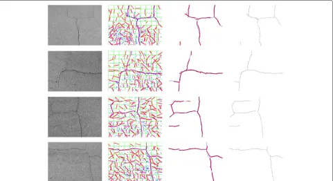
Figure5illustrates how the proposed approach is able to cope with cracks of different width and depth (making the crack more or less dark) and with background texture.
Due to the camera tilt, the background textons are much more prominent in the lower part of the image (cf. 1stline example for instance) creating numerous false alarms at pixel level (blue pixels in the images of the second column of Fig.5). The local analysis captures the non stationarity
of such a noise (caused by textons) by selecting the most significant elementary strips within local windows (red segments in the images of the second column of Fig.5). However, most of theelementary stripsare false alarms at global scale. Then, the global analysis allows for their fil-tering by checking their consistency at image scale (red segments in the third column versus the second column in Fig.5). Finally, having detected the rough shape of the cracks, the post-processing step allows for a finer estima-tion of the shape as well as removal of some isolated false alarms. Note also that the local analysis is important not only to improve the resilience to texture nonstationarity, but also to crack width variations. For instance, the sec-ond row illustrates the ability of the method to recover not only the main cracks, but also the thinner ones: the win-dow scale step allows for local significance maximization, whereas the sole use of a global measure would have esti-mated thin cracks to be insignificant relatively to wider cracks.
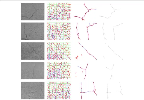
On Fig.6, examples have been chosen to illustrate the limits of the proposed approach. Three main phenomena
induce adverse conditions for cracks detection: the short-ness of some crack subparts, the thinshort-ness of the crack, and an apparent partial occlusion of the crack. The first phenomenon is illustrated for instance on the two first rows of Fig.6, where some branches of a main crack are missed because they do not present a sufficient length to be considered as significant. The second phenomenon is illustrated on the two last rows of Fig. 6, where the thinness of some crack subparts makes them almost invis-ible. However, in these examples (as in many others, although it is not always the case), the post-processing allows for the reconnection of the actually detected crack subparts. The third phenomenon is illustrated on the third and the fifth rows of Fig. 6, where in some places the crack has been partially filled by the background mate-rial inducing a kind of occlusion of the crack. Then, like in the case of the crack of extreme thinness, some crack parts are missed at the end of the global scale analysis. Note also that the fifth row case is particularly adverse since it combines both thinness and partial occlusion problems.
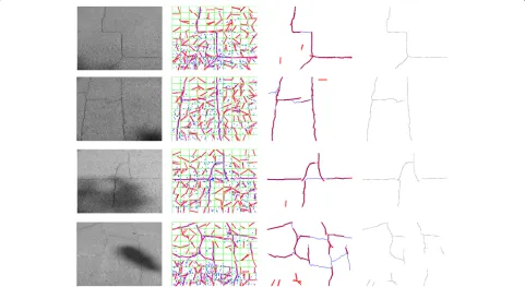
Figure 7 presents results on images with a shadow introducing an adverse effect which increases from first to last rows. Indeed, in the 1st and 2nd line cases, the presence of the shadow affects only the global distribu-tion of gray level values which, according to the shown results, does not actually impact the algorithm
perfor-mance. The result shown on the 3rd row allows us to
check the robustness to illumination non stationarity induced by the shadow, whereas the result shown on the 4throw stresses the limit of this robustness. Indeed, in the 3rd row case, the local analysis is still able to detect the crack in the shadowed part (because local con-trast remains even if attenuated), while in the 4th row case the darkness of the shadow removes some subparts of the crack that cannot be recovered based on align-ment criterion because of the “alligator-skin” feature of the crack. This cases are particularly challenging since alligator cracks tend to form complex patterns in terms of crack directions with ramifications which partially contradicts our assumption that cracks are fine, linear structures.
In summary, we evaluate our algorithm with respect to five adverse phenomena for crack detection: two phe-nomena that are independent of the cracks themselves, namely the background texture and the shadow presence, and three phenomena that characterize the cracks, namely the thinness, the length of secondary branch(es), and the
partial filling (behaving like partial occlusion). The anal-ysis of the results shows that, even in presence of these adverse phenomena, the algorithm is able to detect almost every strip that composes the actual cracks, and follow their jagged behavior. The window level detection allows us to remove most false alarms introduced at pixel level (seeds), but introduces some window level false alarms (on average, one detection per window is not related to an actual crack) which are then removed by the image scale detection, unless they are found to belong to a significant strip at image level.
4.2 Impact of the scale on the local analysis
In Algorithm 2, the scale of the local analysis is driven by the window size. This parameter depends on the image resolution as well as on the sinuosity of the structures to detect, so that it is up to the user to define its value. How-ever, to illustrate its importance, we study its impact with respect to our specific application and data.
Figure8illustrates the influence of different choices of window sizes, firstly on the elementary strip detection and then on the significant straight chain detection. As expected, for large windows (160×120), elementary strips are able to capture the underlying crack with an approxi-mation which is rather coarse yet robust. On the contrary,
in the presence of small windows (40×30), elementary
strips succeed in better following the crack sinuosity but
Fig. 8Qualitative impact of the window size. Illustration on elementary strips (1stline, red borders) and on significant straight chains of elementary strips (2ndline, red pixels): data image and ground truth are shown in 1stcolumn; window size varies in{160×120; 80×60; 40×30}from 2ndto 4thcolumn; also shown: seed pixels (1stline, blue color), post-processing result (2ndline, blue pixels)
are prone to lack of significance. For instance, the zig-zag shape of the crack in the lower left part of the image is not captured at a coarse window resolution (while being well followed using finer windows), and the less contrasted crack in the right part of the image is missed using too small window resolution (while being well detected using larger windows). Finally, the post-processing step results, obtained by cost path minimization strongly guided by straight chain approximation (blue curves in the second
line of Fig.8), present a final refinement and correct some local misdetections.
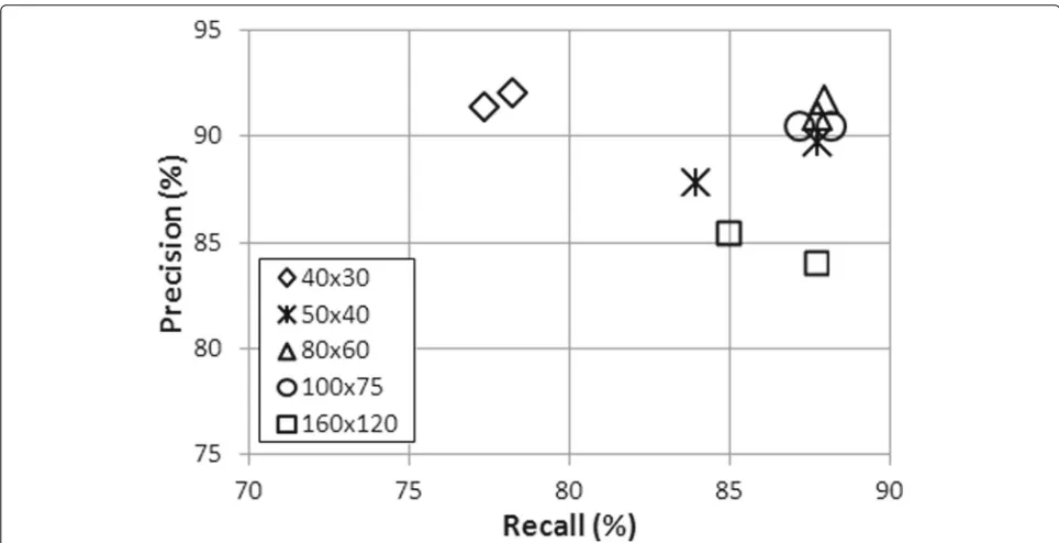
In order to add also a quantitative evaluation of scale of local analysis, Fig.9shows the performance indices (pre-cision and recall) obtained considering five window sizes, namely {40×30; 50×40; 80×60; 100×75; 160×120}. Besides, two different seed images have been consid-ered to draw more robust conclusions. These two seed images correspond to more or less strict criteria in the
Fig. 10Running time evaluation. Statistics (in terms of percentiles) versus the window size parameter for the two main steps of Algorithm 2:
adetection of elementary strips (window level) andbdetection of significant straight chains of elementary strips (image level)
preprocessing step [30] so that the number of seeds in the binary image input of Algorithm 2 varies. Each plotted point corresponds to the average performance computed on a set of 50 images. We note that results are glob-ally in agreement with qualitative comments derived from Fig. 8: smaller window detections lead to few false pos-itives (but possibly more false negatives), thus resulting in better precision value than recall value, whereas using larger windows allow for low false-negative rate and thus higher recall value. However, we note that very similar performances have been obtained for medium window sizes (∈ {80×60; 100×75}), and even for an unoptimal window size, the algorithm exhibits a desirable behavior of graceful degradation in performance.
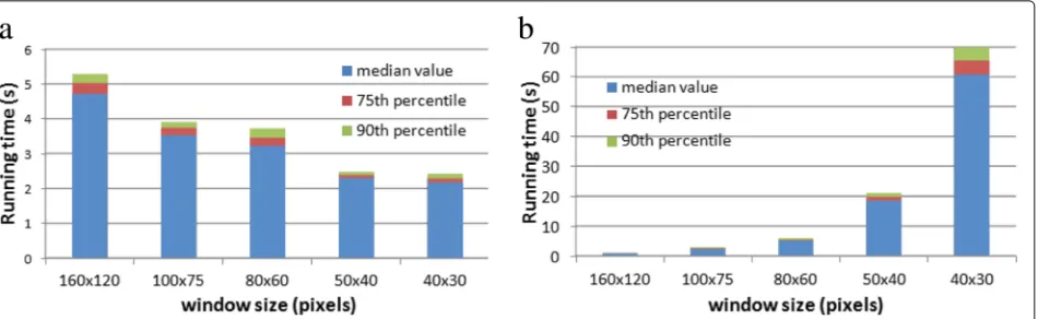
Finally, Fig. 10presents the variation of running time versus window size parameter. We distinguish between the two main steps of the proposed crack detection algo-rithm, namely the detection of elementary strips (step 1) and the detection of significant straight chains of elemen-tary strips (step 2). Even if step 1 could be parallelized in an optimized implementation, as the operations at win-dow level are performed independently, the winwin-dows are processed sequentially in our implementation. However, despite this absence of parallel processing, the running time values are less than a few seconds with a weak depen-dency on the window size: there exists indeed an almost linear dependency between the window size and the time needed for its processing, but at the same time, we observe an inverse proportionality with respect to the number of window to process. Regarding step 2, the window size has a strong impact on the running time, e.g., the median value increases exponentially from 0.8 to 60saccording to our experiments. However, for the chosen window size parameter (80×60 pixels, cf. Section4), the running time is also in the range of a few seconds. Finally, we under-line that these processing times have been obtained on a standard laptop computer (Core i7 [email protected],
4Go RAM), and that better running time perfor-mance may be expected after code optimization and parallelization.
5 Conclusion
In this paper, a generic method for the NFA criterion com-putation for pattern detection is proposed. We consider that relying on an advantageous grouping of parame-ters in the engendered cumulative space is applicable to a wide variety of problems and may facilitate the use of a-contrario based algorithms for various applications involving parametric pattern detection. Our technique was applied to a crack detection task, which naturally fits the problem as cracks can be seen as a deviation from the naive model in a heterogeneous background, allowing us to illustrate the pertinence and the benefit of re-parametrization and multi-scale a-contrario analysis for complex patterns.
Future work will be devoted to accelerating the accu-mulation tasks, since most cumulative space operations are inherently independent and could therefore take advantage of parallel architectures. On such architectures (GPU, FPGA), the available memory resources are often more constrained than on generic systems. However, the reduced memory footprint resulting from our algorithm should be directly beneficial in such scenario.
Abbreviations
FPGA: Field-programmable gate array; GPU: Graphics processing unit; NFA: Number of false alarms
Acknowledgements
We would like to acknowledge the support from the authors of [26] for providing the dataset for benchmarking and for various discussions.
Funding
This work has been funded by authors’ own resources.
Availability of data and materials
The crack image dataset [26] used for the experiments is publicly available at
Authors’ contributions
SLH designed and conceived the research and implemented the core algorithm. SLH, EA, and JV performed the experiments and analyzed the experimental results. SLH and EA drafted the manuscript. All authors read and approved the final manuscript.
Competing interests
The authors declare that they have no competing interests.
Publisher’s Note
Springer Nature remains neutral with regard to jurisdictional claims in published maps and institutional affiliations.
Received: 13 July 2018 Accepted: 17 January 2019
References
1. A. Desolneux, L. Moisan, J.-M. Morel, Meaningful alignments. Int. J. Comput. Vis.40(1), 7–23 (2000)
2. A. Desolneux, L. Moisan, J.-M. Morel, A grouping principle and four applications. IEEE Trans. Pattern. Anal. Mach. Intell.25(4), 508–513 (2003) 3. R. G. Von Gioi, J. Jakubowicz, J.-M. Morel, G. Randall, On straight line
segment detection. J. Math. Imaging Vis.32(3), 313 (2008) 4. R. G. von Gioi, J. Jakubowicz, J.-M. Morel, G. Randall, LSD: A fast line
segment detector with a false detection control. IEEE Trans. Pattern. Anal. Mach. Intell.32(4), 722–732 (2010)
5. C. Akinlar, C. Topal, Edlines: A real-time line segment detector with a false detection control. Pattern. Recogn. Lett.32(13), 1633–1642 (2011) 6. A. Almansa, A. Desolneux, S. Vamech, Vanishing point detection without
any a priori information. IEEE Trans. Pattern Anal. Mach. Intell.25(4), 502–507 (2003)
7. J. Lezama, R. Grompone von Gioi, G. Randall, J.-M. Morel, inProceedings of the IEEE Conference on Computer Vision and Pattern Recognition. Finding vanishing points via point alignments in image primal and dual domains (IEEE, Columbus, 2014), pp. 509–515
8. A. Newson, A. Almansa, Y. Gousseau, P. Pérez, Robust automatic line scratch detection in films. IEEE Trans. Image Process.23(3), 1240–1254 (2014)
9. J. Lezama, J.-M. Morel, G. Randall, R. G. Von Gioi, A contrario 2d point alignment detection. IEEE Trans. Pattern. Anal. Mach. Intell.37(3), 499–512 (2015)
10. S. Blusseau, A. Carboni, A. Maiche, J. Morel, R. G. von Gioi, Measuring the visual salience of alignments by their non-accidentalness. Vis. Res.126, 192–206 (2016)
11. C. Akinlar, C. Topal, Edcircles: A real-time circle detector with a false detection control. Pattern. Recog.46(3), 725–740 (2013)
12. V. P˘atr˘aucean, P. Gurdjos, R. G. von Gioi, Joint a contrario ellipse and line detection. IEEE Trans. Pattern. Anal. Mach. Intell.39(4), 788–802 (2017) 13. T. Veit, F. Cao, P. Bouthemy, An a contrario decision framework for
region-based motion detection. Int J Comput. Vis.68(2), 163–178 (2006) 14. N. Burrus, T. M. Bernard, J.-M. Jolion, Image segmentation by a contrario
simulation. Pattern. Recognit.42(7), 1520–1532 (2009)
15. J. Rabin, J. Delon, Y. Gousseau, A statistical approach to the matching of local features. SIAM J. Imaging Sci.2(3), 931–958 (2009)
16. A. Robin, L. Moisan, S. Le Hégarat-Mascle, An a-contrario approach for subpixel change detection in satellite imagery. IEEE Trans. Pattern Anal. Mach. Intell.32(11), 1977–1993 (2010)
17. G. Palma, I. Bloch, S. Muller, Detection of masses and architectural distortions in digital breast tomosynthesis images using fuzzy and a contrario approaches. Pattern Recognit.47(7), 2467–2480 (2014) 18. S. Zair, S. Le Hégarat-Mascle, E. Seignez, A-contrario modeling for robust
localization using raw GNSS data. IEEE Trans. Intell. Transp. Syst.17(5), 1354–1367 (2016)
19. P. V. Hough, Method and means for recognizing complex patterns. Google Patents. US Patent 3,069,654 (1962)
20. F. Porikli, inComputer Vision and Pattern Recognition, 2005. CVPR 2005. IEEE Computer Society Conference On, vol. 1. Integral histogram: A fast way to extract histograms in cartesian spaces (IEEE, San Diego, 2005), pp. 829–836 21. F. Dibos, S. Pelletier, G. Koepfler, inImage Processing, 2005. ICIP 2005. IEEE
International Conference On, vol. 1. Real-time segmentation of moving objects in a video sequence by a contrario detection (IEEE, Genova, 2005), p. 1065
22. F. Dibos, G. Koepfler, S. Pelletier, Adapted windows detection of moving objects in video scenes. SIAM J. Imaging Sciences.2(1), 1–19 (2009) 23. S. Chambon, J.-M. Moliard, Automatic road pavement assessment with image
processing: Review and comparison. Int. J. Geophys.2011, 1–20 (2011) 24. T. Yamaguchi, S. Hashimoto, Fast crack detection method for large-size concrete surface images using percolation-based image processing. Mach. Vis. Appl.21(5), 797–809 (2010)
25. Y. Fujita, Y. Hamamoto, A robust automatic crack detection method from noisy concrete surfaces. Mach. Vis. Appl.22(2), 245–254 (2011)
26. Q. Zou, Y. Cao, Q. Li, Q. Mao, S. Wang, CrackTree: Automatic crack detection from pavement images. Pattern. Recognit. Lett.33(3), 227–238 (2012) 27. J. Vandoni, S. Le Hégarat-Mascle, E. Aldea, inPattern Recognition (ICPR),
2016 23rd International Conference On. Crack detection based on a marked point process model (IEEE, Cancún, 2016), pp. 3933–3938
28. N. Batool, R. Chellappa, inEuropean Conference on Computer Vision. Modeling and detection of wrinkles in aging human faces using marked point processes (Springer, Florence, 2012), pp. 178–188
29. S.-G. Jeong, Y. Tarabalka, J. Zerubia, inImage Processing (ICIP), 2014 IEEE International Conference On. Marked point process model for facial wrinkle detection (ICIP, Paris, 2014), pp. 1391–1394
30. E. Aldea, S. Le Hégarat-Mascle, Robust crack detection for unmanned aerial vehicles inspection in an a-contrario decision framework. J. Electron. Imaging.24(6), 061119–061119 (2015)
31. T. S. Nguyen, S. Begot, F. Duculty, M. Avila, inImage Processing (ICIP), 2011 18th IEEE International Conference On. Free-form anisotropy: A new method for crack detection on pavement surface images (ICIP, Brussels, 2011), pp. 1069–1072
32. L. Qingquan, Z. Qin, Z. Daqiang, Q. Mao, FoSA: F* seed-growing approach for crack-line detection from pavement images. Image Vis. Comput.
29(12), 861–872 (2011)
![Table 2 Main statistical values on precision and recall indexesachieved on the CrackTree dataset [26]](https://thumb-us.123doks.com/thumbv2/123dok_us/876011.1585093/9.595.306.539.110.220/table-statistical-values-precision-recall-indexesachieved-cracktree-dataset.webp)