A New 3D Empirical Plastic and Damage Model for Simulating the Failure of Concrete Structure

ORIGINAL ARTICLE

A New 3D Empirical Plastic and Damage

Model for Simulating the Failure of Concrete

Structure

Yan‑tao Jiao

_{, Bo Wang}

_{and Zhen‑zhong Shen}

Abstract

A new plastic–damage constitutive model based on the combination of damage mechanics and classical plastic theory was developed to simulate the failure of concrete. In order to explain different material behaviors of concrete under tensile and compressive loadings, the plastic yield criterion, the different kinematic hardening rule for tension and compressive and the isotropic flow rule were established in the effective stress space. Meanwhile, two different empirical damage evolution equations were adopted: one for compression and the other for tension. A multi‑axial damage influence factor was also introduced to fully describe the anisotropic damage of concrete. Finally, the model response was compared with a wide range of experiment results. The results showed that the model could well describe the nonlinear behavior of concrete in a complex stress state.

Keywords: concrete, plastic–damage model, anisotropic damage, multi‑axial damage influence factor, tensile damage, compressive damage

© The Author(s) 2019. This article is distributed under the terms of the Creative Commons Attribution 4.0 International License (http://creat iveco mmons .org/licen ses/by/4.0/), which permits unrestricted use, distribution, and reproduction in any medium, provided you give appropriate credit to the original author(s) and the source, provide a link to the Creative Commons license, and indicate if changes were made.

1 Introduction

This study mainly aimed to formulate a new plastic–dam-age constitutive model for concrete as completely and as simply as possible.

Existing plastic–damage models (PDMs) of concrete are usually based on sound thermodynamic principles (Hesebeck 2001; Mahnken 2002; Voyiadjis and Deliktas 2000; Cicekli et al. 2007; Taqieddin et al. 2012; Voyiadjis et al. 2008; Abu Al-Rub and Kim 2010; Wu et  al. 2006; Liu et  al. 2013; Mazars and Pijaudier-Cabot 1989; Lee and Fenves 1998). The thermodynamics-based damage model conforms to rigorous mechanical inference and has a solid theoretical foundation, therefore, it is called the theoretical plastic–damage model. Similar to the traditional plastic mechanics theory, a damage criteria and a damage dissipation potential function are needed to set up these models. However, it is hard to define the

damage dissipation potential. In order to simplify the derivation of the model, some authors abandoned the thermodynamics-based damage criteria and turned to the empirically defined ones. One popular pattern of this kind of PDMs is that the models rely on the combina-tion of stress-based plasticity formulated in the effective stress space with a strain-based damage model combined which can be obtained by empirical observations. These works (Grassl and Jir Sek 2006a, b; Grassl et  al. 2013; Kitzig and Häußler-Combe 2011; Murakami 2012; Valen-tini and Hofstetter 2013) belong to this group. The mod-els can be called the empirical plastic–damage modmod-els. As the damage model is based on strain, it may be eas-ily implemented into commonly used strain-driven finite element procedures and the calculation of damage vari-able can be implemented explicitly. Thus, there are robust algorithms for FEM.

However, given the complex anisotropic damage in concrete, some authors adopted a single damage vari-able for both tension and compression (Grassl and Jir Sek 2006a, b; Yu et al. 2010; Kitzig and Häußler-Combe 2011; Valentini and Hofstetter 2013). This is sufficient for monotonic loading with unloading, but it is not suitable

Open Access

*Correspondence: [email protected]

for modeling the transition from tensile to compressive failure (i.e. the unilateral effect and elastic stiffness recov-ery under cyclic loading). In order to overcome this limitation, other authors adopted two isotropic damage variables: one for tension and the other for compres-sion (Grassl et al. 2013; Murakami 2012). In spite of the satisfactory results obtained under the pure tension and pure compression stress states, the anisotropic damage of concrete and the interaction effect of damage in the orthogonal direction under multi-axial stress states were usually neglected in these models. But in fact, the stress-based damage evolution function can also be adopted to formulate the anisotropic constitutive models for quasi-brittle materials which are typical examples (see e.g. Faria et  al. 1998; Berto et  al. 2014). However, in some cases, although axial stress is compression, the corresponding axial strain may be tension or compression. Tensile strain may lead to tensile damage, and in this case, if the stress state is adopted to judge the damage state, the tensile damage may be ignored. Therefore, it is a controversial issue to define that the damage state is compression or tension through the stress state. Though it is also an open question to take strain as a state variable, strain is still used in many models. Moreover, as described by Chal-lamel et al. (2005), damage is mainly a strain-controlled phenomenon. In this paper, we tended to use strain as a state variable to judge the damage state and to establish the damage evolution function.

With inspirations from all the previous works and understandings mentioned above, this paper presented a new PDM for concrete with two different empirical and strain-based damage evolution equations: one for tensile damage and the other for compressive damage. Under multi-axial stress states, the anisotropic damage and the interaction effect of damage in the orthogonal direction were considered and a multi-axial damage influence fac-tor was introduced to extend the uniaxial damage evo-lution equation to a multi-axial form. As shown by Abu Al-Rub and Voyiadjis (2003), Cicekli et  al. (2007) and Abu Al-Rub and Kim (2010), the plastic part of coupled plastic–damage model formulated in the effective space was numerically more stable and attractive. Thus in this paper, the plastic part of the proposed model was estab-lished in the effective stress space. Meanwhile, in order to simplify the derivation of constitutive equations and to bring advantages to the numerical implementation, the strain equivalence hypothesis was adopted in this paper. In addition, for the PDMs, the calibration of the mate-rial parameters usually relies on monotonic stress–strain experimental curves, but this results in a non-unique determination of the material parameters. Therefore, a simple and effective method which needs the uniax-ial cyclic loading stress–strain experimental curves to

identify the material parameters was proposed by Abu Al-Rub and Kim (2010). However, since the uniaxial cyclic tests are relatively complex, the stress–strain data is usually obtained by uniaxial monotonic test in actual engineering. Therefore, the method proposed by Abu Al-Rub and Kim (2010) to determine the material param-eters may cause the lack of uniaxial cyclic loading stress– strain data. In order to overcome this limitation, a new method for the calibration of the material parameters was proposed in this paper.

Finally, a new empirical plastic and anisotropic dam-age model for plain concrete was formulated here. In the model, different responses of concrete under tension and compression were considered, including the effect of stiffness degradation, the interaction effects of damage in the orthogonal direction and the stiffness recovery due to crack closure in cyclic loading. To demonstrate the capa-bility of the proposed model, the model response was compared with a wide range of experimental results.

2 Theoretical Basics of Plastic‑Damage Model 2.1 Damage Part

2.1.1 Definition of Damage Variable

According to Rabotnov (1968), the relation between the nominal stress and the effective stress can be expressed as:

where

where A , AD and A¯ respectively denote the whole area, the total damage area and the effective area. d denotes the isotropic damage variable which varies from 0 to 1. The sign ( ) denotes the physical quantity of the effec-tive configuration corresponding to the nominal configu-ration ( ).

Similarly, if the isotropic damage model is adopted under multi-axial stress state, the relation between the effective stress tensor σ¯ and the nominal stress tensor σ can be expressed as follows:

By cutting out the section to determine the amount of holes, cracks and to accumulate the amount, the dam-age density of material can be directly determined, i.e. the damage variable d can be determined by Eq.  (2). However, it is very difficult to put it into practice. In order to indirectly determine the damage density and simplify the derivation of constitutive equations, the strain equivalence hypothesis was proposed by Lemaitre

(1)

¯

σ = σ

1−d

(2) d= A− ¯A

A = AD

A

(3) ¯

and Chanboche (1974). Based on the strain equivalence hypothesis, the total nominal strain tensor ε can be set

equal to the corresponding effective strain tensor ε¯ , which can be decomposed into an elastic strain εe(= ¯εe ) and a plastic strain εp ( = ¯εp ), such that:

It should be noted that the original formulation of the strain equivalence hypothesis only applies to the elastic strain, i.e. one can only assume that the nominal elastic strain tensor εe is equal to the corresponding effective elastic strain tensor ε¯e . However, as described by Abu Al-Rub and Voyiadjis (2003) and Cicekli et  al. (2007), the additional permanent strain caused by damage in the nominal configuration was minimal and could be neglected. In this paper, the nominal plastic strain tensor εp was assumed to equal the corresponding effective plas-tic strain tensor ε¯p . For simplicity, in this form, the strain equivalence hypothesis was used in these works, see e.g. Lee and Fenves (1998), Cicekli et  al. (2007); Wu et  al. (2006), Abu Al-Rub and Kim (2010), Liu et  al. (2013), Grassl and Jir Sek (2006a), Grassl et al. (2013), Murakami (2012), Faria et al. (1998) and Al-Rub et al. (2013).

Based on Eqs. (3), (4) and the generalized Hook’s law, the stress–strain relationship can be expressed as:

where E is the fourth-order damaged elastic stiffness ten-sor, which is a function of the damage variable d and E is the fourth-order initial undamaged elastic stiffness ten-sor. For isotropic linear-elastic material, E is given by:

where G= ¯E0/2(1+ ¯ν) and K = ¯E0/3(1−2ν)¯ are respectively the effective shear and bulk moduli with _E¯₀ being the initial Young’s modulus and ν¯ being the Pois-son’s ration.

Based on Eq. (5), the indirect form of damage vari-able expressed by stiffness degradation can be shown as follows:

For the case of one-dimension, the above equation can be rewritten as:

where E is the damaged Young’s modulus.

It is assumed in isotropic damage that the strength and stiffness of the concrete material are equally degraded (4) ε=εe+εp=ε¯e+ε¯p=ε¯

(5)

σ =E:εe=E:(ε−εP)=(1−d)E¯ :(ε−εP)

=(1−d)E¯ _{: ¯}εe=(1−d)σ¯

(6) Eijkl=2Gδikδjl+

K−2

3G

δijδkl

(7)

d=1−E_{: ¯}E−1

(8)

d=1− E ¯

E0

in different directions upon damage evolution, but this is not the fact. In order to capture the load-induced ani-sotropy of concrete, the second-order symmetric damage tensor ωij was adopted in this paper. Matrix representa-tion of the tensor ωij in the principal axes is as follows:

where ωˆi, i=1, 2, 3 represents the eigenvalues and can be expressed as:

In the subsequent development, the superscript hat symbol (ˆ•) denotes a principal value of (•).

Ei is an unknown quantity to be determined by the strain-based damage evolution function.

2.1.2 Damage Evolution Function

Since damage is an irreversible process, in this paper, the damage evolution function was described by the damage loading equations, loading–unloading conditions and the evolution laws for damage variables. In addition, given that the damage mechanisms of concrete behave differ-ently in tension and compression, to better describe the different damage mechanisms under tensile and com-pressive loadings, two different empirical and strain-based damage evolution equations were adopted in this paper. Hereafter, the superscripts “+” and “−” respec-tively denote the tensile and compressive entities.

1. Uniaxial damage evolution function

The uniaxial damage (i.e. isotropic damage) load-ing functions and loadload-ing–unloadload-ing conditions can be expressed as:

where f_d± is the axial loading function, εˆ±(σˆ¯±) is the axial strain and k_d± is the axial damage-driven history variable which is used to store the maximum value that the axial strain can reach. Therefore, the axial damage-driven history variable k_d± never decreases even when the

(9) �

ωij�= 



ˆ

ω1 ˆ

ω2 ˆ

ω3





(10) ˆ

ωi =1− Ei ¯ E0

, i=1, 2, 3

(11)

f_d±=βεˆ±(σˆ¯±)−k_d±

(12) k_d±=βεˆ±(σˆ¯±),β=

1 if εˆ+≥0

−1 if εˆ−<0

corresponding axial strain εˆ±(σˆ¯±) decreases in the load-ing process.

The significance of damage loading functions and load-ing–unloading conditions can be simply interpreted as: if

f_d±<0 and the material is in the cyclic loading or elastic unloading state, damage evolution cannot occur because the condition in Eq. (13) implies that _k˙±

d =0 . If f

± d =0 , the material can exhibit damage evolution characterized by _k˙±

d >0.

Since both damage and plastic deformations lead to the nonlinear response of concrete, both of the two deforma-tions should be taken into account. For uniaxial tensile and compressive loading, σˆ¯+ and σˆ¯− are given as (Lee and Fenves 1998)

where εˆ±p is the axial plastic strain which can be expressed by εˆ±p=t

0εˆ˙±pdt.

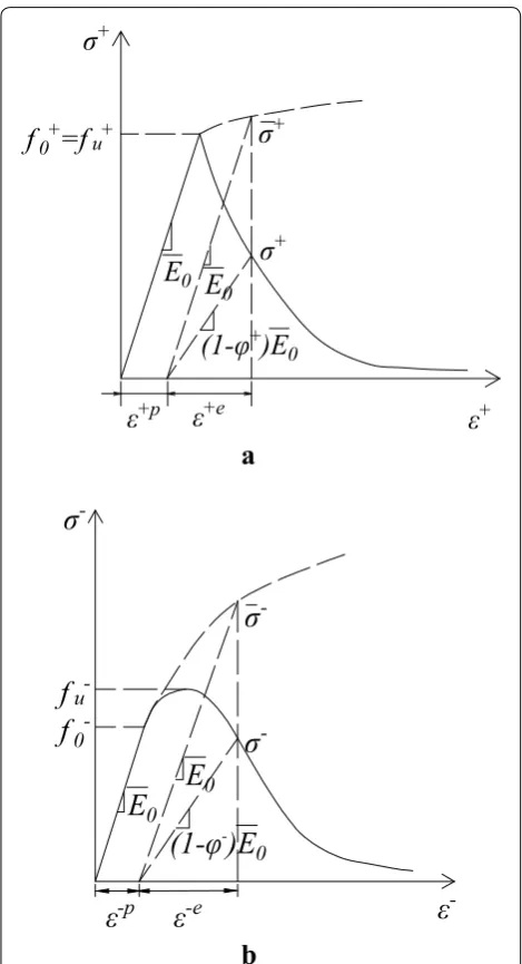
In this paper, the Guo-Zhang model recommended by code for design of concrete structure (GB50010-2002) (Ministry of Construction 2002) was adopted to express the stress–strain relation of concrete under the uniaxial stress state. For uniaxial tensile loading, the relation between stress and strain can be expressed as follows:

where xˆ+= ˆε+/ε₀+ , αt=0.312(f₀+)2 , f₀+ is the uniaxial tensile strength and ε₀+ is the strain corresponding to f₀+ . ε₀+ and Aˆ+ can be obtained by the following expression:

where αt is the material parameter and can be obtained by the following equation:

From Eq.  (16), it is known that f₀+ is a cut-off point and before the point, material is linear-elastic and after the point, material shows nonlinear feature, i.e. the mate-rial response seems to be weakened as the plastic strain increases because the elastic stiffness of the material is degraded due to damage evolution after the cut-off point (see Fig. 1a).

(14) ˆ

σ+=(1−d+)σˆ¯+=(1−d+)E¯0εˆ+e

=(1−d+)E¯0(εˆ+− ˆε+p)

(15) ˆ

σ−=(1−d−)σˆ¯−=(1−d−)E0¯ εˆ−e =(1−d−)E0¯ (εˆ−− ˆε−p)

(16)

ˆ

σ+=f₀+

1.2ˆx+−0.2ˆx+6

if xˆ+≤1 ˆ

σ+=f₀+Aˆ+ if xˆ+>1

(17) ε₀+=

f₀+0.54

×65×10−6,

ˆ

A+= ˆx+/

αtxˆ+−11.7+ ˆx+

(18) α_t=0.312(f₀+)2

Setting Eq. (14) equal to Eq. (16) and using k_d+ to replace εˆ+ in Eqs. (14) and (16), the solving for d+ will be:

For uniaxial compressive loading, the relation between stress and strain can be expressed as follows:

(19) d+=

 



0 if k_d+≤ε+₀

1− ε

+

0Aˆ+

(k_d+−ˆε+p₎ if k

+ d > ε

+ 0

(20)

 



ˆ

σ−=�_¯ E0ε−u

�

ˆ

x− if xˆ−≤0.211 ˆ

σ−=f_u−Bˆ− if 0.211≤ ˆx−≤1 ˆ

σ−=f_u−Cˆ− ifxˆ−>1

a

b

ε

_ε

_ε

E

(1-φ

_)E

f

=f

E

σ

σ

σ

ε

_ε

ε

-f

-E

E

f

-σ

-σ

-σ

-(1-φ

_)E

0

where xˆ−= ˆε−/ε−_u , f_u− is the uniaxial compressive strength and ε_u− is the strain corresponding to f_u− . ε−_u , Bˆ− and _Cˆ− _{can be expressed as:}

where αa and αd are the material parameters which can be obtained by the following equations:

From Fig. 1b, it can be seen that damage and plasticity are caused when the applied stress reaches f₀−=0.4f_u−

under uniaxial compressive loading. Therefore, using k_d− to replace εˆ− in Eq. (15), setting Eq. (15) equal to Eq. (20) and solving for d− , the following can be obtained:

where |•| is a symbol of absolute value.

2. Multi-axial damage evolution functioρn

Although uniaxial damage evolution law can reflect the general rule of damage evolution under uniaxial stress state, the mechanical characteristics and damage evolu-tion of concrete are greatly different under multi-axial stress states. And for multi-axial stress states, a more advanced multi-axial damage evolution law is required.

A lot of uniaxial loading experiments of concrete show that the propagation direction of cracks is perpendicu-lar to the stress direction under uniaxial tensile loading and cracks are parallel to the loading direction under compressive loading. Therefore, for uniaxial tensile load-ing, the damage evolution direction is consistent with the stress direction, which can be called “direct damage”. But for uniaxial compressive loading, the damage evo-lution direction is vertical to the stress direction, which can be called “indirect damage”. According to the experi-ment results of these works (Peng et  al. 1997; Kupfer et al. 1969; Gao et al. 2001), the compressive strength of concrete in biaxial compressive states was significantly higher than the strength in uniaxial compressive state; under biaxial tensile–compressive states, the tensile strength of concrete in one direction obviously decreased

(21) ε−_u =

700+172

fu−

×10−6,

ˆ

B−=αaxˆ−+(3−2αa)xˆ−2+(αa−2)xˆ−3,

ˆ

C−= ˆx−/

αd

ˆ

x−−12

+ ˆx−

(22) αa=2.4−0.0125fu−,

α_d =0.157

f_u−0.785−0.905

(23)

d−=     

   

0 if 0≤k_d−<��0.211ε_u−

� �

1− |fu−|Bˆ−

¯

E0(k−d−|ˆε−p|)

if ��0.211ε−_u

�

�≤k_d−< � �ε−_u

� �

1− |fu−|Cˆ−

¯

E0(k−d−|ˆε−p|) if �

�ε−_u � �≤k−

d

with the increase of compressive stress (or strain) in the orthogonal direction, and the effect on the compressive strength in one direction due to the tensile stress (or strain) in the orthogonal direction was not very obvi-ous. However, under biaxial tensile states, the variation of the tensile strength caused by tensile stress (or strain) in the orthogonal direction was very small. Based on these experiment results, it was assumed that: (1) com-pressive strain affected the tensile or comcom-pressive dam-age in the orthogonal direction; (2) tensile strain did not affect the damage in the orthogonal direction. According to this assumption, a multi-axial damage influence factor was introduced to extend the uniaxial damage evolution equation to a multi-axial form.

The multi-axial damage loading functions and loading– unloading conditions can be expressed as:

where f_d(i) is the axial loading function, εˆi(σˆ¯i) is the axial

strain, k_d(i) is the axial damage-driven history variable and

i=1, 2, 3.

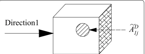
As it is shown in Fig. 2, assuming that the total damage in direction 1 is made up of many micro circular crack areas _A˜D

1j , the total damage area in direction 1 can be expressed as:

where A1 is the whole cross-sectional area and A¯1 is the effective load-carrying area.

Based on Eq. (2), neglecting the effect of strain in the orthogonal direction, the damage variable in direction 1 can be expressed as d1= ˜AD1/A1.

According to the linear-elastic fracture mechanics theory, in an infinite medium, including elliptical micro-cracks, there will be shear stress at the crack tip under

(24) f_d(i)=βiεˆi(σˆ¯i)−k_d(i)

(25) k_d(i)=βiεˆi(σˆ¯i),βi =

1 ifεˆi≥0 −1 ifεˆ_i<0

(26)

f_d(i)≤0,k˙_d(i)≥0,k˙_d(i)f_d(i)=0

(27) ˜

AD₁ =A˜D_1j=A1− ¯A1

A

Direction1

uniaxial compressive loading and this will make the crack extend. It can be noted from Fig. 3 that if direction 1 is tensile strain and direction 2 is compressive strain (i.e. tension–compression combination), new crack exten-sion will occur under the effect of compressive strain, and this will lead to the increase of the total damage area in direction 1 and will produce new damage. If setting the diameter of a damaged region _A˜D

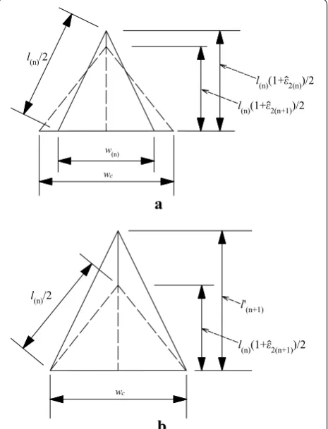
1j in direction 1 at load-ing step n as l(n) and the compressive strain in direction 2 as εˆ2(n) , with the effect of compressive strain εˆ2(n) taken into account, the diameter of the damaged region _A˜D

1j will reduce from l(n) to l(n)(1+ ˆε2(n)) . Based on the geo-metrical relationship of Fig. 4a, the crack width w(n) can be expressed as follows:

with εˆ2(n)<0.

Furthermore, it can be noticed from Fig. 4a that wc is a critical crack width. With the increase of the compressive strain εˆ2(n) , the diameter of the damaged region A˜D1j will further decrease from l(n)(1+ ˆε_2(n)) to l(n)(1+ ˆε₂(n+1)) . When the opening crack width w(n) reaches wc , new crack propagation will occur. At this moment, it can be seen from Fig. 4b that the length of the crack will extend from l(n)(1+ ˆε2(n+1)) to l

′

(n+1) . Based on the geometrical rela-tionship of Fig. 4b, w(n+1) can be expressed as:

with εˆ2(n+1)<0.

And the extended area of the damage region _A˜D

1j can be

derived as:

where AD_1j is the extended area of the damage region A˜D_1j. Based on Eq.  (30), the extended total damage area in direction 1 can be expressed as:

(28)

w(n)=

−ˆε2(n)(2+ ˆε2(n))l(n)

(29) w(n+1)=wc=

−ˆε2(n+1)(2+ ˆε2(n+1))l(n)

(30)

AD_1j= ˜AD_1jw

2

(n+1)

ˆ ε2(n+1)

w2_(n) ˆ ε2(n)

(εˆ2(n+1)<0)

where AD₁ is the total damage area in direction 1 when the effect of εˆ2 is considered and A˜D₁ is the total damage area in direction 1 when the effect of εˆ2 is neglected.

According to the above definition of damage variable and with the effect of compressive strain εˆ2 considered, the new damage ωˆ1 in direction 1 at step n+1 can be derived as:

where d1(n+1)

ˆ ε1(n+1)

is the damage in direction 1 at step n+1 without considering the effect of εˆ2 and χ2(n+1) is the tensile damage influence factor caused by compres-sive strain in direction 2 at step n+1.

(31) AD₁ =AD_1j= w

2

(n+1)

ˆ

ε2(n+1)

w2_(n)

ˆ

ε2(n)

˜

AD_1j

= w 2

(n+1)

ˆ

ε2(n+1)

w2_(n)εˆ2(n) A˜

D

1 (εˆ2(n+1)<0)

(32)

ˆ

ω1(n+1)=

AD₁ A1

=d1(n+1)

ˆ ε1(n+1)

w

2

(n+1)

ˆ ε2(n+1)

w2_(n) ˆ ε2(n)

=d1(n+1)

ˆ ε1(n+1)

χ2(n+1) (εˆ2(n+1)<0)

l

ε2

Direction 1

Direction 2

Crack

Crack

l(1+ε2), ε2<0

Fig. 3 Sketches of crack opening under compressive strain in direction 2.

a

b

l_(n)/2

l_(n)(1+ε_2(n))/2

wc w_(n)

l_(n)(1+ε_2(n+1))/2

l'_(n+1)

wc

l_(n)(1+ε_2(n+1))/2 l_(n)/2

Fig. 4 The geometrical relationship between crack width and length.

Similarly, if direction 3 is also compressive strain, the damage in direction 1 can be written as follows:

As mentioned earlier, it is difficult to

deter-mine the damage variable by Eq.  (2) (i.e.

di=(Ai− ¯Ai)/Ai(i=1, 2, 3) ), thus, to determine the damage density indirectly, the strain equivalence hypoth-esis was proposed by Lemaitre and Chanboche (1974). This means that Eq. (2) is equivalent to Eq. (8), such that:

It should be noted that the uniaxial tensile damage evolution equation  (19) is derived on the basis of the strain equivalence hypothesis (i.e. d=1−E/E0¯ ). Based on Eqs. (33, 19) can be extended to a multi-axial form as follows:

with i,j=1, 2, 3 , and χ_j can be expressed as:

When both direction 1 and direction 2 are compres-sive strain, the area of damage region in direction 1 will show a shrinking tendency due to the effect of compres-sive strain in direction 2, and the damage density in direc-tion 1 will decrease. Therefore, a multi-axial compressive damage influence factor χ_i′ for compression-compression combination should be defined. Since the reduction of the damage density in direction 1 caused by the compressive strain in direction 2 was not very obvious, after repeated trials, the multi-axial compressive damage influence fac-tor χ_i′ was assumed as a constant and 0.8 was used in the study. Substituting χ_i′ into Eq. (23), the multi-axial com-pressive damage evolution equation is shown as follows:

(33) ˆ

ω1(n+1)=d1(n+1)εˆ1(n+1)χ2(n+1)χ3(n+1)

×(εˆ2(n+1)<0,εˆ3(n+1)<0)

(34) di= Ai− ¯Ai

Ai

= A˜ D i Ai

=1− Ei ¯ E0

(35)

ˆ ω_i+=

 



0 if k_d+(i)≤ε+₀

� 1− ε

+ 0Aˆ+i

(kd+(i)−ˆε

+p i )

� 3 Π

j=1χj if k +(i) d > ε

+ 0

(36) χj=

−

ˆ

εj+�ˆεj(2+ ˆεj+�ˆεj) −ˆεj(2+ ˆεj)

ˆ εj<0.

(37) ˆ

ω_i−=        

      

0 if 0≤k_d−(i)<��0.211ε−_u� � �

1− |fu−|Bˆ−i

¯

E0(k−(i)d − � � �εˆ

−p i

� � �)

� 3 Π j=1

χ_j′

χ_i′ if �

�0.211ε−_u� �≤k

−(i) d <

� �ε_u−��

�

1− |fu−|Cˆ − i

¯

E0(k−(i)d − � � �εˆ

−p i

� � �)

� 3 Π j=1

χ_j′

χ_i′ if � �ε_u−��≤k

−(i) d

with i,j=1, 2, 3.

2.1.3 Stiffness Degradation

1. Definition of Damaged Elastic Stiffness with Cyclic Loading Neglected

The degradation of stiffness caused by damage occurs in both tension and compression and becomes more significant as the strain increases. Since the anisotropic damage tensor was adopted in this paper, Eq. (3) can be extended as:

As described by Murakami (2012), the effective stress tensor obtained by Eq.  (38) was asymmetric. Since it is usually inconvenient to use the asymmetric effective stress tensor in the formulation of constitutive and evo-lution equations, several symmetrization methods were proposed by many authors. The method proposed by Cordebois and Sidoroff (1982) is used frequently (Carol et  al. 2001; Prochtel and Häußler-Combe 2008; Mozaf-fari and Voyiadjis 2015; Murakami 2012). By this method, Eq. (38) can be rewritten as follows:

or

where

In the principal coordinate system of damage ω with the Voigt notations, the fourth-order damage-effect ten-sor M can be expressed as the following “diagonal matrix form”:

where φ_i=1− ˆω_i with ωˆ_i(i=1, 2, 3) being the principal damage variable.

(38) ¯

σ =(I−ω)−1σ.

(39) ¯

σ =(I−ω)−1/2σ(I−ω)−1/2

(40) σ =M(ω): ¯σ

(41) Mijkl=

1 2

(δ_ik −ω_ik)1/2(δ_jl−ω_jl)1/2

+(δil−ωil)1/2(δjk−ωjk)1/2 .

(42)

M₍ω_ˆ)=digφ

1 φ2 φ3

φ₂φ₃

As described by Chow and Wang (1987), since the fourth-order damage-effect tensor Mijkl contained more individual components and the elements in a fourth-order tensor were difficult if not impossible to be measured, the simplification became necessary for practical reasons. Zhu and Cescotto (1995), Chow and Wang (1987) and Zhang et al. (2001) used the simplified damage effect tensor in Eq. (42) to establish the relation between the effective and nominal stress tensors, and the matrix representation of the nominal stress tensor can be written as:

where

and

with Ei=φiE¯0 , Eij =

φ_iφ_jE0¯

i,j=1, 2, 3

and ̟ =1/(1+ ¯ν)(1−2ν)¯ .

Combining Eqs. (14), (15) and (43)–(45), it can be seen that the principal nominal stress can be expressed as:

When a single damage variable for both tension and compression is adopted, the pattern of stiffness degrada-tion defined in Eq. (45) will be applicable, e.g. Kitzig and Häußler-Combe (2011). However, if two different dam-age variables for tension and compression are adopted, in some cases, it may be inappropriate to establish the constitutive relationship. Taking the true tri-axial com-pressive test reported by Van Mier (1984) as an example, when the stress ratio was σˆ1/σˆ2/σˆ3= −1/−0.1/−0.05 , only εˆ1 was compressive strain and both εˆ2 and εˆ3

were tensile strains. In this case, the negative and positive principal nominal stress components were

ˆ

σ−=σˆ−

1 , 0.1σˆ1−, 0.05σˆ1− T

and σˆ+=(0, 0, 0)T . And the corresponding negative and positive principal strain components can be written as εˆ−=εˆ−

1, 0, 0

T

and ˆ

ε+=0,εˆ+

2,εˆ3+

T

. By using the damaged elastic stiffness (43) {σ} =[E]

ε−εp =[E]

εe

(44)

{σ} =

σ11 σ22 σ33 σ23 σ13 σ12T

{ε} =

ε11 ε22 ε33 ε23 ε13 ε12T

(45) [E]=̟·

       

E1(1− ¯ν) E1ν¯ E1ν¯ 0 0 0

E2ν¯ E2(1− ¯ν) E2ν¯ 0 0 0

E3ν¯ E3ν¯ E3(1− ¯ν) 0 0 0

0 0 0 E23(1₂−2ν)¯ 0 0 0 0 0 0 E13(1₂−2ν)¯ 0 0 0 0 0 0 E12(1₂−2ν)¯

        (46) ˆ

σ_i=φ_i

¯ K+4

3G¯

ˆ ε_ie+φ_i

¯ K−2

3G¯

3

j=1

ˆ ε_je.

tensor defined in Eq.  (45), the principal nominal stress vector can be expressed as:

Obviously, when a single damage variable for both ten-sion and compresten-sion is adopted, the above equation is reasonable. But when two different damage variables are adopted, Eq. (47) can be rewritten as:

It can be seen that the mixing term φ+

ˆ

ε+

· ˆ¯σ− in Eq.  (48) is in conflict with Eqs.  (14), (15) and it cannot reflect the different damage mechanisms under tensile

and compressive loadings. In order to eliminate the mix-ing term and to include the unilateral effect, the spectral decomposition technique can be used to separate the stress or strain tensor into positive and negative compo-nents. If the spectral decomposition of the stress tensor is performed, based on the assumption that the expres-sion in Eq. (40) is valid for both tension and compression, such that:

Then the total nominal stress tensor can be expressed as:

And Eq. (47) can be rewritten as:

(47)    ˆ σ₁ ˆ σ₂ ˆ σ₃    =   φ1 � ˆ ε1 �

φ2�εˆ2� φ3 � ˆ ε3 �      ˆ¯ σ₁ ˆ¯ σ₂ ˆ¯ σ₃    . (48)    ˆ

σ₁−

ˆ

σ₂−

ˆ

σ₃−

   =  

φ₁−� ˆ

ε−₁�

φ₂+� ˆ

ε₂+�

φ+₃� ˆ

ε₃+�      ˆ¯

σ₁−

ˆ¯

σ₂−

ˆ¯

σ₃−

 

 .

(49) σ+=M+ω+: ¯σ+, σ−=M−ω−: ¯σ−.

(50) σ =M+ω+: ¯σ++M−ω−: ¯σ−.

(51)    ˆ σ₁ ˆ σ₂ ˆ σ₃    =  

1 0 0

0 φ₂+�

ˆ ε+₂�

0

0 0 φ+₃�

ˆ ε₃+�

     0 0 0    +  

φ₁−�εˆ₁−� 0 0

0 1 0

0 0 1

     ˆ¯ σ₁−

ˆ¯ σ₂−

ˆ¯ σ₃−

 



From the above equation, it can be seen that the mix-ing term is eliminated, but a new issue is introduced (i.e.

ˆ

σ₂= ˆ¯σ₂− and σˆ₃= ˆ¯σ₃− ). Obviously, due to the character-istics of the damage evolution equations defined in this paper, the spectral decomposition of the stress tensor is unsuitable for this study. Therefore, the strain tensor will be separated into positive and negative components in the paper. By using the spectral decomposition tech-nique, the following relation can be obtained:

where I_ijkl=P_ijkl+ +P_ijkl− is the fourth identity tensor and

where H(x) is the Heaviside step function ( H(x)=1 for

x>0 and H(x)=0 for x<0 ), εˆ(k) is the kth principal strain of ε and n(k)

i is the kth corresponding unit principal direction.

Since the normalized eigenvector of the elastic tensor is identical to the normalized eigenvector of the total strain tensor, the positive and negative parts of the elastic strain tensor can be expressed as:

Therefore, the elastic strain tensor can be expressed as:

Based on Eqs.  (5) and (54), the positive and negative effective stress tensors can be expressed as follows:

Based on Eq. (40), it is shown that E₌M_{: ¯}E . Since M is a function of ε , the positive and negative nominal stress tensors can be expressed as follows:

Then, the nominal stress tensor can be expressed as: (52)

ε_ij+=P_ijkl+ εkl, ε−ij =(Iijkl−P_ijkl+ )εkl =P_ijkl− εkl

(53)

P+_ijkl=

3

k=1

H(εˆ(k))n(_ik)n_j(k)n(_kk)n(_lk)

(54)

ε+e=P+:εe=P+:ε−εp

ε−e=P−:εe=P−:ε−εp

.

(55)

εe=I:εe=P++I−P+:εe

=P+_:εe+P−:εe=ε+e+ε−e

.

(56)

¯

σ+= ¯E:P+:(ε−εp)= ¯E:ε+e

¯

σ−= ¯E:P−:(ε−εp)= ¯E:ε−e

(57)       

σ+=M+�ε+�:σ¯+=M+�ε+�:E¯ :ε+e

=E+�

ε+�:ε+e=E+�ε+�:P+:(ε−εp) σ−=M−�ε−�:σ¯−=M−�ε−�:E¯ :ε−e

=E−�

ε−�:ε−e=E−�ε−�:P−:(ε−εp)

.

(58)

σ =σ++σ−=E+ε+:ε+e+E−ε−:ε−e.

In order to make it easy to write program, the above equation in matrix form can be written as:

with

E±

ε±

being the positive and negative dam-aged elastic stiffness matrixes which can be obtained by Eq. (45).

By the above method, Eq. (47) can be then rewritten as:

with Υ being expressed as:

and Ψ being expressed as:

By rearranging the above three equations, the following equation can be obtained:

From Eq. (63), it can be seen that when using the pat-tern of stiffness degradation defined in Eq. (45) and com-bining the spectral decomposition of the strain tensor to establish the constitutive relationship, although the result was improved, there were still some issues, i.e. the effec-tive stress components σˆ¯₁+ , σˆ¯₂− and σˆ¯₃− could not degrade into nominal stress.

In order to overcome this limitation, a different pattern of stiffness degradation should be defined. To take the effective principal or normal stress in any principal direc-tion as the resultant force of the axial stresses in three orthogonal directions, i.e.

with ̟ (1− ¯ν) and ̟ν¯ being contributing coefficient, and assuming that when damage occurs and the axial effec-tive stresses degrade into nominal stresses, with the nom-inal principal or normal stress in any principal direction being the resultant force of the axial nominal stresses, i.e.

(59) {σ}=

E+ ε+

ε+e +

E− ε−

ε−e . (60)    ˆ σ₁ ˆ σ₂ ˆ σ₃   

=̟E¯0(Υ +Ψ ).

(61) Υ =





(1− ¯ν) ν¯ ν¯

φ₂+ν¯ φ+₂(1− ¯ν) φ+₂ν¯

φ₃+ν¯ φ₃+ν¯ φ₃+(1− ¯ν)      0 ˆ

ε₂+

ˆ

ε₃+    . (62) Ψ =  

φ−₁(1− ¯ν) φ₁−ν¯ φ₁−ν¯ ¯

ν (1− ¯ν) ν¯ ¯

ν ν¯ (1− ¯ν)

     ˆ ε−₁

0 0    . (63)    ˆ σ₁ ˆ σ₂ ˆ σ₃    =  

1 0 0

0 φ+₂ 0

0 0 φ₃+

     ˆ¯

σ₁+

ˆ¯

σ₂+

ˆ¯

σ₃+    +   φ₁− 0 0

0 1 0 0 0 1

     ˆ¯

σ₁−

ˆ¯

σ₂−

ˆ¯

σ₃−    . (64)    ˆ¯ σ₁ ˆ¯ σ₂ ˆ¯ σ₃    =̟ ·   

(1− ¯ν)σˆ¯₁′ + ¯νσˆ¯₂′ + ¯νσˆ¯₃′ ¯

νσˆ¯₁′ +(1− ¯ν)σˆ¯₂′ + ¯νσˆ¯₃′ ¯

νσˆ¯₁′ + ¯νσˆ¯₂′ +(1− ¯ν)σˆ¯₃′

 

with σˆ_i′ =φiσˆ¯

′

i(i=1, 2, 3),then the matrix representation of damaged elastic stiffness tensor can be defined as:

By this method, Eq. (47) can be rewritten as:

where Υ′ can be expressed as:

and Ψ′ can be expressed as:

By rearranging the above three equations, the following equation can be obtained:

From Eq. (70), it can be noted that the issue existing in Eq. (63) was avoided.

Through further analysis, it is seen that Eq. (66) can be decomposed as:

where _¯ E

is the initial undamaged elastic stiffness matrix and [M] can be expressed by Eq. (42).

Then Eq. (59) can be rewritten as:

(65)    ˆ σ₁ ˆ σ₂ ˆ σ₃    =̟ ·   

(1− ¯ν)σˆ₁′ + ¯νσˆ₂′ + ¯νσˆ₃′ ¯

νσˆ₁′+(1− ¯ν)σˆ₂′ + ¯νσˆ₃′ ¯

νσˆ₁′+ ¯νσˆ₂′ +(1− ¯ν)σˆ₃′  



(66)

[E]=̟·

       

E1(1− ¯ν) E2ν¯ E3ν¯ 0 0 0

E1ν¯ E2(1− ¯ν) E3ν¯ 0 0 0 E1ν¯ E2ν¯ E3(1− ¯ν) 0 0 0

0 0 0 E23(1₂−2ν)¯ 0 0

0 0 0 0 E13(1₂−2ν)¯ 0

0 0 0 0 0 E12(1₂−2ν)¯

        . (67)    ˆ σ₁ ˆ σ₂ ˆ σ₃    =̟ � Υ′+Ψ′ � . (68) Υ′ =  

(1− ¯ν) φ+₂ν¯ φ₃+ν¯ ¯

ν φ₂+(1− ¯ν) φ₃+ν¯ ¯

ν φ+₂ν¯ φ₃+(1− ¯ν)      0 ˆ¯ σ₂′+

ˆ¯ σ₃′+

   . (69) Ψ′ =  

φ₁−(1− ¯ν) ν¯ ν¯ φ−₁ν¯ (1− ¯ν) ν¯ φ−₁ν¯ ν¯ (1− ¯ν)

     ˆ¯ σ₁′−

0 0    . (70)    ˆ σ₁ ˆ σ₂ ˆ σ₃    =̟·     

φ₂+ν¯σˆ¯₂′++φ₃+ν¯σˆ¯₃′++φ−₁(1− ¯ν)σˆ¯₁′− φ₂+(1− ¯ν)σˆ¯₂′++φ₃+ν¯σˆ₃′++φ₁−ν¯σˆ¯₁′− φ₂+ν¯σˆ¯₂′++φ₃+(1− ¯ν)σˆ¯₃′++φ₁−ν¯σˆ¯₁′−

     . (71)

[E]=_¯

E [M]

(72) {σ}=_¯

E

M+ ε+e

+_¯

E

M− ε−e

where

M±(ωˆ±) can be expressed as:

where φ_i±=(1− ˆω_i±)2 with ωˆ_i±(i=1, 2, 3) being the principal tensile and compressive damage variables.

The damage–effect matrix shown in Eq. (73) is in the principal coordinate system of damage which corre-sponds to the direction of the principal strains. In terms of a general coordinate system, it should be transformed to the global coordinate system as following:

where [R] is the coordinate transition matrix.

By substituting Eq.  (74) into Eq.  (72), Eq.  (72) can be rewritten as:

2. Definition of damaged elastic stiffness for cyclic loading

Tests of concrete showed that the degradation of the elastic stiffness had unilateral effect under cyclic loading due to the opening and closing of micro cracks caused by the load that changed the sign during the loading process. It can be explained that some tensile cracks tended to close when the load changed from tension to compression, which led to elastic stiffness recovery dur-ing compressive loaddur-ing; whereas, in the case of transi-tion from compression to tension, the pre-existing cracks formed during the previous compressive loading and the new cracks formed during the subsequent tensile load-ing would cause further reduction of the elastic stiffness. Because the damage-effect matrix

M_∗±

defined in Eq. (75) did not include the elastic stiffness recovery phe-nomenon, the formulation proposed by Lee and Fenves (1998) for cyclic loading was extended in this paper for the anisotropic damage.

When the load changes from compression to tension, the anisotropic tensile damage variable will be assumed as follows:

(73)

M±

=digφ₁± φ±₂ φ±₃

φ±₂φ±₃

φ±₁φ±₃

φ₁±φ₂±

(74)

M_∗±

ˆ

ω

=[R]T M±

[R]

(75)

{σ}=_¯

E M+_∗

ε+e+_¯ E

M_∗− ε−e.

(76)

ˆ

where wˆ+_i is the tensile damage variable for cyclic load-ing and H(x) is the Heaviside step function ( H(x)=1 for

x>0 and H(x)=0 for x<0).

For the case of transition from tension to compression, the anisotropic compressive damage variable is defined as:

where wˆ_i− is the compressive damage variable for cyclic loading and 0≤s0≤1 is a constant. Any value between 0

and 1 will result in partial recovery of the elastic stiffness. Based on Eqs. (76) and (77), the following can be obtained:

a. when all principal strains are positive, H(ˆεi)=1 and Eq. (76) becomes

which implies that there is no stiffness recovery occurs when the load changes from compression to tension.

b. when all principal strains are negative, H(εˆ_i)=0 and H(−ˆε_i)=1 and Eq. (76) can be simplified down to

ˆ

w_i+=0 , then Eq. (77) becomes

which can reduce to wˆ_i−= ˆω_i− when s0=0 , and

it implies full elastic stiffness recovery during the transition from tension to compression. If s0=1 , Eq.  (79) will reduce to the form of Eq.  (78), which means that there is no stiffness recovery. For the case of 0<s0<1 , Eq.  (79) can be written as

ˆ

w_i−=s0ωˆ+i + ˆωi−−s0ωˆ+i ωˆ−i , and it can be explained that some tensile cracks tend to close or partially close and as a result, elastic stiffness partial recovery occurs in compressive loading. To simplify the cal-culation, in this paper, the value of s0 was set to one, i.e. full elastic stiffness recovery during the transition from tension to compression.

As mentioned above, if εˆ1>0 , εˆ2<0 and εˆ3<0 , then the following can be obtained:

By substituting wˆ_i+ and wˆ_i− into

M±

defined in Eq. (73), the damage-effect matrix for cyclic loading can be rewritten as follows:

(77) ˆ

w_i−=1−(1−H(−ˆεi)s0ωˆ−_i )(1−H(−ˆεi)ωˆ−_i )

(78)

ˆ

w_i+=1−(1− ˆω+_i )(1− ˆω−_i )= ˆω+_i + ˆω_i−− ˆω+_i ωˆ_i−

(79)

ˆ

w_i−=1−(1−s0ωˆ_i+)(1− ˆω−_i )

(80)

ˆ

w₁+= ˆω+₁ + ˆω−₁ − ˆω₁+ωˆ−₁, wˆ₁−=0

ˆ

w₂+=0, wˆ₂−=s0ωˆ2++ ˆω2−−s0ωˆ2+ωˆ−2

ˆ

w₃+=0, wˆ₃−=s0ωˆ3++ ˆω3−−s0ωˆ3+ωˆ−3 .

where ϑ_i+=(1−H(ˆεi)ωˆ_i+)(1−H(ˆεi)ωˆ_i−) and

ϑ_i−=(1−H(−ˆεi)s0ωˆ+_i )(1−H(−ˆεi)ωˆ−_i ) with ωˆ_i+ and ωˆ−_i being respectively the principal tensile and compressive damage variables and i=1, 2, 3.

Combining Eqs. (71), (74) and (81), the final form of the damaged elastic stiffness for cyclic loading can be expressed as:

2.2 Plasticity Part

Concrete has different material behaviors under tensile and compressive loadings, thus the yield criterion proposed by Lubliner et  al. (1989) that accounts for both tension and compression plasticity was adopted in this work. This cri-terion was successful in simulating the concrete behavior under uniaxial, biaxial, multiaxial and cyclic loadings (Lee and Fenves 1998; Yu et al. 2010; Cicekli et al. 2007; Abu Al-Rub and Kim 2010; Shen et al. 2015). Furthermore, it was proved by Abu Al-Rub and Voyiadjis (2003) that PDMs for-mulated in the effective space were numerically more stable and attractive. In many works, this strategy was adopted (Abu Al-Rub and Kim 2010; Grassl et  al. 2013; Liu et  al. 2013; Murakami 2012), so was in this paper. Thus the yield criterion proposed by Lubliner et al. (1989) is expressed in the effective configuration as follows:

where J2= ¯sij¯sij/2 is the second-invariant of the effective deviatoric stress tensor ¯sij= ¯σij− ¯σkkδij/3 , I1= ¯σkk is the first-invariant of the effective Cauchy stress tensor σ¯_ij ,

ˆ¯

σmax is the maximum principal effective stress, H(σˆ¯max) is the Heaviside step function, and the parameters α and β are dimensionless constants which are defined by Lubliner et al. (1989) as follows:

with fb0 and f0− being respectively the initial equi-biax-ial and uniaxequi-biax-ial compressive yield stress. Experimental values for fb0/f0− lie between 1.10 and 1.16 and yielding

values for α are between 0.08 and 0.12. Referring to Abu

Al-Rub and Kim (2010) 0.12 was chosen as the value for α in this study.

(81)

M_C± ˆ w±_i

=digϑ₁±ϑ₂±ϑ₃±

ϑ₂±ϑ₃±

ϑ₁±ϑ₃+

ϑ₁±ϑ₂±

(82)

E±_C

=_¯ E

[R]TM±_C

[R].

(83) f =

3¯J2+α¯I1+β(k_ip)H(σˆ¯max)

−(1−α)c¯−(ε−_eq)≤0

(84) α= (fb0/f

− 0 )−1 2(fb0/f0−)−1

, β=(1−α)c¯ −_(ε−

eq) ¯ c+_(ε+

eq)

The internal plastic state variable k_ip in Eq. (83) can be defined as follows:

with its rate being expressed as

or

where H+ and H− are defined as

and

The dimensionless parameter r(σˆ¯ij) is a weight factor which can be expressed as follows:

where the sign �•� indicates Macauley bracket, which is defined as

In fact, ε˙_eq+ and ε˙−_eq are equivalent to the following two equations:

and

where εˆ˙pmax and εˆ˙pmin are respectively the maximum and minimum eigenvalues of the plastic strain rate ε˙_ijp . If ˆ˙

ε₁p>εˆ˙p₂>εˆ˙₃p , then εˆ˙pmax= ˆ˙εp1 and εˆ˙ p

min= ˆ˙ε

p

3 and εˆ˙

P can be expressed as:

(85) k_ip=

t

0

˙

k_ipdt=

t

0

˙

p_BPσˆ¯

dt

(86) ˙

k_ip=Hijεˆ˙jp

(87)      ˙ ε+_eq

0 ˙ ε−_eq

     =  

H+ 0 0 0 0 0 0 0 H−

         ˆ˙ εP₁ ˆ˙ εP₂ ˆ˙ εP₃

       (88) H+=r(σˆ¯ij)

(89)

H−= −(1−r(σˆ¯ij))

(90) r(σˆ¯_ij)=

3 k=1 ˆ¯ σ_k 3 k=1 σˆ¯k

(91)

�x� = 1

2(|x| +x),k=1, 2, 3.

(92)

˙

ε_eq+ =r(σˆ¯ij)εˆ˙pmax

(93) ˙

ε_eq− = −(1−r(σˆ¯ij))ˆ˙εminp

(94) ˆ˙ ε p = ˆ˙

ε₁p εˆ˙₂p εˆ˙p₃T = ˙P ∂Gpσˆ¯

∂σˆ¯

where GP is the plastic potential, which is to be described later.

Combining Eqs. (87) and (94), the expression Bp(σˆ¯) in Eq. (85) can be obtained as

Since concrete behavior in compression is more of a ductile behavior as compared to its corresponding brit-tle behavior in tension (Abu Al-Rub and Kim 2010), the isotropic hardening expressions c¯+ and ¯c− in the effective configuration are defined as follows:

where _f¯+

0 and f¯0− ( f¯0−<0 ) are respectively the effective yield strengths under uniaxial tension and compression. The parameters Q− , b− and h+ are material constants, which are obtained in the effective configuration of the uniaxial cycle stress–strain diagram.

In view of the material property of concrete, in the present model, the flow rule is given as a function of the effective stress σ¯_ij , such that:

where ˙p is the Lagrangian plasticity multiplier, which can be obtained under the plasticity consistency condi-tion, _f˙_{=0 , such that}

The plastic potential Gp _{adopted in this paper is the} Drucker-Prager function expressed as:

where αp is a parameter chosen to provide proper dis-tance with common range between 0.2 and 0.3 for con-crete, and the plastic flow direction ∂Gp/∂σ¯ij in Eq. (100) can be expressed as

(95) Bp�σˆ¯

� =     r � ˆ¯ σ � 0 0

0 0 0

0 0 −�1−r�σˆ¯ ��     · ∂Gp � ˆ¯ σ � ∂σˆ¯ . (96) ¯

c+= ¯f₀++h+ε+_eq

(97)

¯

c−= −¯f₀−+Q−

1−exp(−b−ε_eq−)

(98) ˙

ε_ijp= ˙p∂G

p

∂σ¯ij

(99)

f ≤0,˙p_≥0,˙p_{f =0,}˙p_f˙_=0.

(100) Gp=

3¯J2+αpI¯1

(101) ∂Gp

∂σ¯ij

= 3 2

¯ sij

3J¯2

3 Calibration and Comparisons with Test Results To investigate the applicability and effectiveness of the proposed model, several numerical examples of con-crete under different loading conditions were presented in this section. The model response was compared with five groups of experiments including cyclic, uniaxial, and biaxial loading.

The calibration of the material parameters often relies on monotonic stress–strain experimental curves. How-ever, this method results in a non-unique determina-tion of these material parameters. Therefore, based on the uniaxial cyclic test, Abu Al-Rub and Kim (2010) proposed a method to identify the plasticity material parameters. The method can be summarized as follows: Firstly, the damaged Young’s module E for each cycle can be determined by connecting each unloading points ( A−E ) and reloading points ( A′−E′ ) shown in Fig. 5. Then the effective stress σ¯ can be obtained by the equa-tion as σ¯ =(E¯/E)σ . Under this condition, the plasticity parameters h+ , Q− and b− can be determined. Moreover, from Eq. (8) and the measured damaged Young’s module in Fig. 5, the variation of the damage density with strain can be plotted shown in Fig. 6b such that d=1−E/E¯0 . For more details of this method, Abu Al-Rub and Kim (2010) can be referred. As mentioned previously, since the uniaxial cyclic tests are relatively complex, the stress– strain data is usually obtained by uniaxial monotonic test in actual engineering. Therefore, the method proposed by Abu Al-Rub and Kim (2010) to identify the plasticity parameters may cause the lack of uniaxial cyclic load-ing stress–strain data. Based on the above analysis, the following method was used to identify the plasticity parameters in this study, and it can be summarized as

follows: Firstly, based on Eqs. (16) and (20), the relations between stress and strain under uniaxial stress state can be obtained. With Eqs. (19) and (23), the damage vari-ables d+ and d− can be determined. However, since the axial plastic strains ε±p are unknowns in the computing processes of the damage variables d+ and d− , in order to obtain the damage variables, the axial plastic strains should be determined firstly. As discussed in Zhang et al. (2008), the ratio of axial plastic strain ε+p and ine-lastic strain ε+ck under uniaxial tension can be taken as

0.50−0.95 and the ratio of axial plastic strain ε−p and ine-lastic strain ε−in under uniaxial compression can be taken as 0.35−0.70 . As shown in Fig. 1, the inelastic strains ε+ck and ε−in can be obtained by the following equations:

(102) ε+ck =ε+−σ+/E¯0, ε−in=ε−−σ−/E¯0.

Fig. 5 Experimental stress–strain curves in the effective and nominal configurations for Karsan and Jirsa (1969) experimental data.

In this study, based on the experimental results of uni-axial cyclic tensile test of Taylor (1992) and uniaxial cyclic compressive test of Karsan and Jirsa (1969), the ratio of axial plastic strain ε+p and inelastic strain ε+ck was taken as 0.90 , and the ratio of axial plastic strain ε−pand inelas-tic strain ε−in was taken as 0.60 . With this, the damage variables d′+ and d′− by using Eqs. (19) and (23) can be obtained, and then the effective stress σ¯ can be obtained by using Eq. (1). Based on the above analysis, the plastic-ity material parameters can be obtained by fitting the cal-culated effective stress-axial plastic strain curve.

3.1 Uniaxial Cyclic Compressive Test

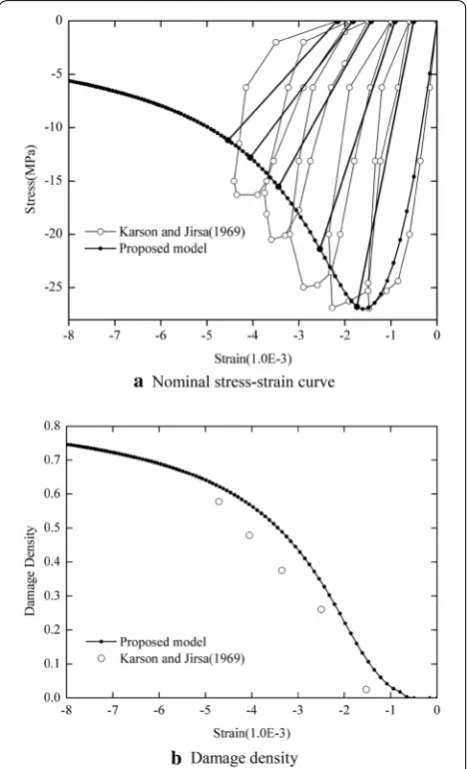
Using the method mentioned above, the identified com-pressive plasticity and damage material constants asso-ciated with fitting Karsan and Jirsa (1969) experimental data are listed in Table 1. The comparison between the numerical predictions and the experiment results is shown in Figs. 5 and 6.

From Fig. 5, it can be seen that the predicted effective stress–strain curve is in line with the experiment result. However, Fig. 6a shows that the predicted nominal stress Table 1 Material constants identified from the experimental

results (Karsan and Jirsa 1969).

E0(Gpa) ν f_u− (MPa) ε−_u

(1.0E−3)

31.00 0.20 − 27.00 −1.59

α_a α_d Q−(MPa) b−

2.06 1.18 74.00 702.14

Table 2 Material constants identified from the experiment

results of Taylor (1992).

E0(Gpa) ν f+

0(MPa)

31.00 0.2 3.40

ε+₀(1.0E−4) αt h+(MPa)

1.26 3.61 4436

Fig. 7 The model responses in cyclic tension compared to experimental results presented in Taylor (1992).

Table 3 Material properties used for  the  monotonic

uniaxial compressive test.

E0(Gpa) ν f_u−(MPa) ε−_u

(1.0E−3)

31.70 0.20 −27.63 −1.60

αa α_d Q−(MPa) b−

2.05 1.22 37.00 3173

is slightly smaller than the experiment result. The main reason is that the predicted damage density is higher than the value showed in the experiment result under the same strain (see Fig. 6b). Although the damage density is slightly higher than the predicted value, the calculated result is reasonable because the bigger predicted damage value is safer in project.

3.2 Uniaxial Cyclic Tensile Test

With the same method mentioned above, the identified material parameters are listed in Table 2. The experi-ment results of uniaxial cyclic tensile test of Taylor (1992) are compared with the numerical predictions shown in Fig. 7. From Fig. 7, it can be seen that the predicted nom-inal stress–strain curve and the damage density agree with the experiment results.

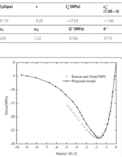
3.3 Monotonic Uniaxial Compressive Test

The experiment results of uniaxial compressive test (Karsan and Jirsa 1969) were employed in this paper for comparison. The material properties adopted in the sim-ulation are listed in Table 3. The comparison between the simulation and test is presented in Fig. 8. From Fig. 8, it can be seen that the predicted nominal stress is slightly smaller than the value showed in the experiment result. This phenomenon is also caused by the bigger predicted damage density.

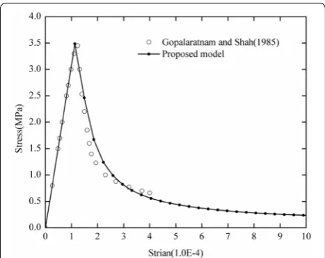
3.4 Monotonic Uniaxial Tensile Test

The comparison between the numerical predictions and the experimental results of Gopalaratnam and Shah (1985) is presented in Fig. 9. The material con-stants used in this simulation are listed in Table 4. As it is shown in Fig. 9, the simulated tensile stress–strain curve agrees with the experimental data.

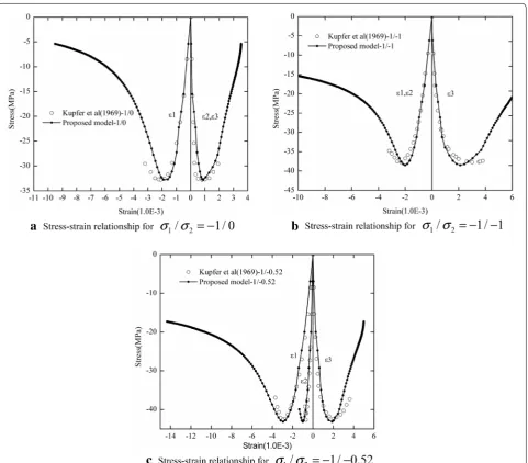
3.5 Monotonic Biaxial Compressive Test

The biaxial compressive test presented in Kupfer et  al. (1969) was adopted in this paper to validate the model. The comparison between the numerical predictions and the experimental results is presented in Fig. 10. The material constants for numerical simulation are listed in Table 5.

In this paper, the strain tensor was decomposed into positive and negative parts by spectrum decomposition technique and the corresponding stress tensor was split into two parts. Through this processing, not only the dif-ferent damage responses can be considered, but also the Poisson’s effect can be easily considered in the biaxial or trial compression test. As it is shown in Fig. 10c, when the biaxial stress ratio is σ1/σ2= −1/−0.52 , bothε1 andε2will be compressive strains and ε3will be the tensile strain. Since tensile strain may lead to tensile damage, to consider tensile material constants is indispensable in this case. This is both an advantage and a disadvantage. The advantage is that the model can accurately charac-terize damage anisotropic of concrete under multi-axial stress state with the Poisson’s effect taken into account, and the disadvantage is that more material constants are needed.

4 Conclusions

Based on the combination of damage mechanics and classical plastic theory, a new empirical plastic–damage constitutive model was presented to simulate the failure of concrete. The proposed model could include different responses of concrete under tension and compression, the effect of stiffness degradation, the interaction effects of damage in the orthogonal direction and the stiffness Fig. 9 The model responses in monotonic uniaxial tension compared

to experimental results presented in Gopalaratnam and Shah (1985).

Table 4 Material parameters used for  the  monotonic uniaxial tensile test.

E0(Gpa) ν _f+

0(MPa)

31.00 0.2 3.45

ε+₀(1.0E−4) α_t h+_(MPa)

recovery due to crack closure in cyclic loading. With comparison with a wide range of experiment results, it was concluded that:

1. The proposed model could effectively simulate the nonlinear properties of concrete under different loading conditions, such as cyclic, uniaxial and biax-ial conditions. Moreover, the proposed model could overcome the limitation of lack of uniaxial cyclic loading stress–strain data in actual engineering and could determine the parameters conveniently.

2. Although choosing strain as the state variable to judge the damage state is a controversial issue, the Fig. 10 The model responses in monotonic uniaxial and biaxial compressive loading compared to experimental results reported by Kupfer et al. (1969).

Table 5 Material constants used for  the  biaxial

compressive test.

Elastic constants Tensile material constants

E0(Gpa) ν _f+

0(MPa) ε +

0(1.0E−4) αt h +_(MPa)

32.00 0.20 2.88 1.15 2.59 8112

Compressive material constants

f−

u(MPa) ε−_u(1.0E−3) αa α_d Q−(MPa) b−

results of simulation in this paper indicated that this choice was feasible. Moreover, although more mate-rial constants are needed with the Poisson’s effect in the multi-axial compressive test being considered, to give an eye to tensile material constants was indis-pensable.

Acknowledgements

The authors are grateful to the support of National Natural Science Founda‑ tion of China (No. 51709116), the Priority Academic Program Develop‑ ment of Jiangsu Higher Education Institutions (No. 3014‑SYS1401), the Key Scientific Research Projects of Henan Province Universities and Colleges (No. 17B570003) and Foundation for Dr in North China University of Water Resources and Electric Power (No. 10030 and 40589). Special thanks for the reviewers and their constructive comments and suggestions in improving the quality of this manuscript.

Authors’ contributions

Z‑ZS conceived and designed the study. Y‑TJ wrote the paper. BW reviewed and edited the manuscript. All authors read and approved the final manuscript.

Competing interests

The authors declare that they have no competing interests.

Author details

1 _{School of Water Conservancy, North China University of Water Resources} and Electric Power, Zhengzhou 450045, China. 2 _{Hohai University, Nan‑} jing 210098, China.

Received: 7 November 2017 Accepted: 6 June 2019

References

Abu Al‑Rub, R. K., & Kim, S. M. (2010). Computational applications of a coupled plasticity–damage constitutive model for simulating plain concrete fracture. Engineering Fracture Mechanics,77, 1577–1603.

Abu Al‑Rub, R. K., & Voyiadjis, G. Z. (2003). On the coupling of anisotropic dam‑ age and plasticity models for ductile materials. International Journal of Solids and Structures,40, 2611–2643.

Al‑Rub, A., Rashid, K., Darabi, M. K., Kim, S.‑M., Dallas, N., Glover, et al. (2013). Mechanistic‑based constitutive modeling of oxidative aging in aging‑ susceptible materials and its effect on the damage potential of asphalt concrete. Construction & Building Materials,41, 439–454.

Berto, L., Saetta, A., Scotta, R., & Talledo, D. (2014). A coupled damage model for RC structures: Proposal for a frost deterioration model and enhancement of mixed tension domain. Construction & Building Materials,65, 310–320. Carol, I., Rizzi, E., & Willam, K. (2001). On the formulation of anisotropic elastic degradation. I. Theory based on a pseudo‑logarithmic damage tensor rate. International Journal of Solids & Structures,38, 491–518.

Challamel, N., Lanos, C., & Casandjian, C. (2005). Strain‑based anisotropic dam‑ age modelling and unilateral effects. International Journal of Mechanical Sciences,47, 459–473.

Chow, C., & Wang, J. (1987). An anisotropic theory of elasticity for continuum damage mechanics. International Journal of Fracture,33, 3–16.

Cicekli, U., Voyiadjis, G. Z., & Abu Al‑Rub, R. K. (2007). A plasticity and anisotropic damage model for plain concrete. International Journal of Plasticity,23, 1874–1900.

Cordebois, J. P., & Sidoroff, F. (1982). Damage Induced Elastic Anisotropy. Dordrecht: Springer, Netherlands.

Faria, R., Oliver, J., & Cervera, M. (1998). A strain‑based plastic viscous–damage model for massive concrete structures. International Journal of Solids and Structures,35, 1533–1558.

Gao, Z.‑G., Huang, D.‑H., & Zhao, G.‑F. (2001). An orthotropic damage constitu‑ tive model for RCC. Journal of Hydraulic Engineering,244, 58–64.

Gopalaratnam, V., & Shah, S. P. (1985). Softening response of plain concrete in direct tension. ACI Journal,82, 310–323.

Grassl, P., & Jir Sek, M. (2006a). Damage‑plastic model for concrete failure. International Journal of Solids and Structures,43, 7166–7196.

Grassl, P., & Jir Sek, M. (2006b). Plastic model with non‑local damage applied to concrete. International Journal for Numerical and Analytical Methods in Geomechanics,30, 71–90.

Grassl, P., Xenos, D., Nystr, M., Rempling, R., & Gylltoft, K. (2013). CDPM2: A dam‑ age–plasticity approach to modelling the failure of concrete. Interna-tional Journal of Solids and Structures,50, 3805–3816.

Hesebeck, O. (2001). On an isotropic damage mechanics model for ductile materials. International Journal of Damage Mechanics,10, 325–346. Karsan, I. D., & Jirsa, J. O. (1969). Behavior of concrete under compressive load‑

ings. Journal of the Structural Division (ASCE),95, 2543–2563.

Kitzig, M., & Häußler‑Combe, U. (2011). Modeling of plain concrete structures based on an anisotropic damage formulation. Materials and Structures,44, 1837–1853.

Kupfer, H., Hilsdorf, H. K., & Rusch, H. (1969). Behavior of concrete under biaxial stresses. Journal of the American Concrete Institute,66, 656–666. Lee, J. H., & Fenves, G. L. (1998). Plastic–damage model for cyclic loading of

concrete structures. Journal of Engineering Mechanics-Asce,124, 892–900. Lemaitre, J. L. & Chanboche, J. L. (1974). A nonlinear model of creep‑fatigue

damage cumulation and interaction. In Proceeding of TUTAM Symposium of Mechanics of Visco-elasticity Media and Bodies, 1974. Gotenbourg: Springer

Liu, J., Liu, R., & Zhong, H. (2013). An elastoplastic damage constitutive model for concrete. China Ocean Engineering,27, 169–182.

Lubliner, J., Oliver, J., Oller, S., & Ate, E. (1989). A plastic–damage model for concrete. International Journal of Solids and Structures,25, 299–326. Mahnken, R. (2002). Theoretical, numerical and identification aspects of a

new model class for ductile damage. International Journal of Plasticity,18, 801–831.

Mazars, J., & Pijaudier‑Cabot, G. (1989). Continuum damage theory—applica‑ tion to concrete. Journal of Engineering Mechanics ASCE,115, 345–365. Ministry of Construction. (2002). Code for design of concrete structures

(GB50010-2002). Beijing: China Building Industry Press.

Mozaffari, N., & Voyiadjis, G. Z. (2015). Phase field based nonlocal anisotropic damage mechanics model. Physica D Nonlinear Phenomena,308, 11–25. Murakami, S. (2012). Continuum damage mechanics: A continuum mechanics

approach to the analysis of damage and fracture. Berlin: Springer. Peng, J., Zhao, G., & Zhu, Y.‑H. (1997). Studies of multiaxial shear strengths for

roller‑compacted concrete. ACI Structural Journal,94, 114–123.

Prochtel, P., & Häußler‑Combe, U. (2008). On the dissipative zone in anisotropic damage models for concrete. International Journal of Solids and structures, 45, 4384–4406.

Rabotnov, Y. N. (1968) Published. Creep rupture. In Proceedings of the XII International Congress on Applied Mechanics, 1968 Stanford. (pp. 342–349). Berlin: Springer

Shen, L., Ren, Q., Xia, N., Sun, L., & Xia, X. (2015). Mesoscopic numerical simulation of effective thermal conductivity of tensile cracked concrete. Construction & Building Materials,95, 467–475.

Taqieddin, Z. N., Voyiadjis, G. Z., & Almasri, A. H. (2012). Formulation and verification of a concrete model with strong coupling between isotropic damage and elastoplasticity and comparison to a weak coupling model. Journal of Engineering Mechanics,138, 530–541.

Taylor, R. (1992). FEAP: A finite element analysis program for engineering worksta-tion. Berkeley: Department of Civil Engineering, University of California. Valentini, B., & Hofstetter, G. (2013). Review and enhancement of 3D concrete

models for large‑scale numerical simulations of concrete structures. International Journal for Numerical and Analytical Methods in Geomechan-ics,37, 221–246.

van Mier, J. G. M. (1984). Strain-softening of concrete under multiaxial loading conditions (Ph.D. Thesis). Eindhoven: Technische Hogeschool Eindhoven. Voyiadjis, G. Z., & Deliktas, B. (2000). A coupled anisotropic damage model

for the inelastic response of composite materials. Computer Methods in Applied Mechanics and Engineering,183, 159–199.

Voyiadjis, G. Z., Taqieddin, Z. N., & Kattan, P. I. (2008). Anisotropic damage–plas‑ ticity model for concrete. International Journal of Plasticity,24, 1946–1965. Wu, J., Jie, L., & Faria, R. (2006). An energy release rate‑based plastic–dam‑