Prediction of railway induced ground vibration through multibody and ﬁnite element modelling

(1)

Mech. Sci., 4, 167–183, 2013 www.mech-sci.net/4/167/2013/ doi:10.5194/ms-4-167-2013

©Author(s) 2013. CC Attribution 3.0 License.

Mechanical

Sciences

Open Access

Prediction of railway induced ground vibration through

multibody and finite element modelling

G. Kouroussis and O. Verlinden

Universit´e de Mons – UMONS, Faculty of Engineering, Department of Theoretical Mechanics, Dynamics and Vibrations, Place du Parc 20, 7000 Mons, Belgium

Correspondence to: G. Kouroussis ([email protected])

Received: 23 November 2012 – Revised: 19 February 2013 – Accepted: 5 April 2013 – Published: 16 April 2013

Abstract. The multibody approach is now recognized as a reliable and mature computer aided engineering tool. Namely, it is commonly used in industry for the design of road or railway vehicles. The paper presents a framework developed for predicting the vibrations induced by railway transportation. Firstly, the vehicle/track subsystem is simulated, on the basis of the home-made C++libraryEasyDyn, by mixing the multibody model of the vehicle and the finite element model of the track, coupled to each other through the wheel/rail contact forces. Only the motion in the vertical plane is considered, assuming a total symmetry between left and right rails. This first step produces the time history of the forces exerted by the ballast on the foundation, which are then applied to a full 3-D FEM model of the soil, defined under the commercial softwareABAQUS. The paper points out the contribution of the pitch motion of the bogies and carbodies which were neglected in previous publications, as well as the interest of the so-called coupled-lumped mass model (CLM) to represent the influence of the foundation in the track model. The potentialities of the model are illustrated on the example of the Thalys high-speed train, riding at 300 km h−1on the Belgian site of M´evergnies.

1 Introduction

After more than 40 yr of research and development, multi-body dynamics simulation has now reached scientific and commercial maturity: several books exist describing well es-tablished methods to build and integrate the equations of mo-tion (G´eradin and Cardona, 2000; Garcia de Jalon and Bayo, 1993; Shabana, 2005; Bauchau, 2011), and commercial soft-ware’s like MSC/ADAMS, SIMPACK or LMS/Virtual.Lab Motionare commonly used in robotics, car or railway indus-try along with other computer-aided engineering tools like fi-nite element. The coupling of multibody systems with other disciplines offers nowadays a rich area of new developments. For example mechatronic systems which need to integrate specific equations related to controllers, actuators or sensors, or biomechanics where behaviour equations of tissues like muscles must be mixed with the ones of the mechanical sys-tem constituted by the skeleton and the limbs. In this paper, we will present a similar application: the multibody model of a vehicle and the finite element model of the track are merged

in order to constitute a framework aiming at predicting the vi-brations induced by railway vehicles. The model is used as a first step: it provides the time history of the forces exerted on the foundation, which are in turn used as inputs in a 3-D finite element of the soil. The complete process is performed in the time domain.

(2)

2 Railway-induced ground vibrations

It is largely admitted that railway transport constitutes a proper solution to traffic congestion and pollution observed in big cities. However, it also brings nuisances that must re-main limited to avoid opposition of the dwellers. Noise and vibrations generated by the vehicle riding on the localized or distributed irregularities of the track are one of the usual reasons of complaint. It is then important to develop techni-cal solutions to mitigate the railway vibrations, ideally from the beginning of the track and vehicle design. This requires reliable simulation tools, able to reproduce with a sufficient accuracy the propagation of vibrations, from the wheel-rail interface to the buildings, through the track and a medium, the soil, fundamentally inhomogeneous and infinite in three directions.

The problem of railway induced vibrations clearly in-volves 3 components: the vehicle, the track (rails, sleepers and ballast) and the soil.

Initially, the vehicle has often been reduced to a simple moving loaded mass (Wang and Zeng, 2004) or eventually a succession of the latter (Lefeuve-Mesgouez et al., 2002). With such a simplification, the origin of vibration lies in the irregular deflection of the track which induces up and down motion of the moving mass: the rail indeed offers a larger rigidity (and then a smaller displacement) above the sleep-ers than between the latter. This effect is sufficient to ex-plain the so-called soil critical speed: when the speed of a train gets above the Rayleigh wave velocity of the superficial layer, it has a tendency to induce large vibrations. This phe-nomenon is generally observed for soft soils. Many works, as those proposed by Kaynia et al. (2000), Takemiya and Bian (2005) or Kouroussis et al. (2012c), have been conducted to reproduce by simulation this phenomenon. However, other sources contribute to the vibration content, among which the track and wheel irregularities and the vehicle dynam-ics. To reproduce this contribution, a more detailed model of the vehicle becomes necessary (Kouroussis et al., 2010). For example, Costa et al. (2011, 2012) have recently identi-fied the influence and relevance of the mechanical properties of the train and have confirmed that the unsprung and semi-sprung masses must be included in the prediction model. In parallel, Kouroussis et al. (2012b) have analysed the vibra-tory effect of the unsprung masses in the specific case of the tramway of Brussels, showing that a modification of the re-silient wheel stiffness notably reduces the ground vibrations when the vehicle is coming up against local rail defects.

The track is usually considered through a finite element model (Knothe and Grassie, 1993; Zhai and Sun, 1994). The rail is built from beam elements while lumped masses rep-resent the sleepers, connected by springs and dampers to the rail and to the ground. One more layer of lumped masses can possibly be added to take into account the effect of the foun-dation in the track model.

Two principal approaches are used to simulate the wave propagation through the soil: the finite element method (FEM) and the boundary element method (BEM). Initially, BEM was preferably used due its natural ability to represent infinite domains and its good computational efficiency when the problem is formulated in the frequency domain (Do Rˆego Silva, 1994). However, the method becomes cumbersome when dealing with complex geometries, while frequency do-main is limited to linear problems. In parallel, the continu-ously increasing power of computers and the development of infinite elements have opened the door to FEM models and it is presently possible to manage fully three-dimensional soil models, either in frequency (Wang et al., 2008) and, more recently in time domain (Kouroussis et al., 2011e). Indeed, Kouroussis et al. (2011d, 2009) have demonstrated that it is possible, in time domain, to alleviate the require-ments in terms of domain and element size simulation. Let us also mention that some authors have developed combined BEM/FEM models (Galv´ın and Dom´ınguez, 2009; Franc¸ois et al., 2009).

3 Railway vibration prediction model

A complete description of the model that we developed for predicting the vibrations induced by railway traffic can be found in Kouroussis et al. (2012a). Its main characteristics are the following:

– The simulation is performed in the time domain and in two successive steps (Fig. 1): firstly the simulation of the vehicle/track subsystem, whose result is the time history of the forces exerted by the track on the soil and, secondly, the simulation of the response of the soil to these forces through a finite element model.

– The vehicle/track subsystem is processed under the home-made frameworkEasyDynand merges the non-linear equations of motion of the vehicle defined as a multibody model and the linear equations of a finite el-ement model of the track. So far, a perfect symmetry has been assumed between left and right sides so that the motion is restricted to the vertical plane.

– The response of the ground is simulated under the com-mercial software ABAQUS. A particular care is given to the definition of the boundary conditions in order to get the best representation of the domain infinity and in particular to avoid wave reflection.

(3)

G. Kouroussis and O. Verlinden: Railway ground vibrations through multibody and FEM 169 G. Kouroussis and O. Verlinden: Railway Ground Vibrations through Multibody and FEM 3

v0

x z

simplified soil layer

step 1

Dynamic study of the vehicle/track subsystem with a

multibody vehicle model moving on a flexible track

tak-ing into account track irregularity. The vehicle/track

motion is simplified in the vertical plane.

step 2

Dynamic study of the soil subsystem where the soil surface forces correspond to the contribu-tion of the ballast reaccontribu-tion, calculated in the first step.

Figure 1.Vehicle/track/soil model, working in two successive steps

known as Winkler foundation, this term being used for con-tinuously supported track and for discrete model as well as), the hypothesis is valid if the soil is sufficiently stiff, which is the case in most of railway lines (Kouroussis et al., 2011e, 2012a). With softer soils, the authors have proposed an en-hanced track model, referred to as the coupled lumped mass model (CLM), which offers a faithful representation of soft soils impedance in the requested frequency range (Kourous-sis et al., 2011b). In this paper, we will focus on the vehi-cle/track model.

4 Vehicle/track model

4.1 Global structure

The developed model merges the equations of motion of the vehicle, which have the form usually encountered in

multi-body system dynamics

Mv(q

v)·q¨v+hv(qv,˙qv,t)=fv(qv,qt,t) (1)

and the equations of the track, represented by a linear finite element model

Mt·q¨

t+Ct·˙qt+Kt·qt=ft(qv,qt,t) (2)

with

– q

vand qtthe vectors gathering the configuration

param-eters of the vehicle and track, respectively;

– Mvand Mtthe mass matrices of the vehicle and track,

respectively;

– h_vthe term gathering the Coriolis, centrifugal and gyro-scopic terms of the vehicle;

www.mech-sci.net Mech. Sci.

Figure 1.Vehicle/track/soil model, working in two successive steps.

models exist therefore combining multibody and finite ele-ment approaches in a single application for vehicle/track/soil analysis (see for example, Connolly et al., 2013).

The prediction model has been used in various practical cases and was successfully confronted to experimental re-sults (Kouroussis et al., 2010, 2011e, 2012b,c, 2013). The main hypothesis in the approach relies in the two step strat-egy which assumes some decoupling between the track and the soil. However, it turns out that the hypothesis is rea-sonable as far as the mechanical impedance of the rail, as seen from the vehicle, is well represented, including the pos-sible dynamic coupling between the sleepers through the soil. With classical track models where the soil is consid-ered only through the stiffness under the sleepers (generally known as Winkler foundation, this term being used for con-tinuously supported track and for discrete model as well as), the hypothesis is valid if the soil is sufficiently stiff, which is the case in most of railway lines (Kouroussis et al., 2011e, 2012a). With softer soils, the authors have proposed an en-hanced track model, referred to as the coupled lumped mass model (CLM), which offers a faithful representation of soft

soils impedance in the requested frequency range (Kourous-sis et al., 2011b). In this paper, we will focus on the vehi-cle/track model.

4 Vehicle/track model

4.1 Global structure

The developed model merges the equations of motion of the vehicle, which have the form usually encountered in multi-body system dynamics

Mv(qv)·q¨v+hv(qv,˙qv,t)= fv(qv,qt,t) (1)

and the equations of the track, represented by a linear finite element model

Mt·q¨t+Ct·˙qt+Kt·qt= ft(qv,qt,t) (2)

with

– qvand qtthe vectors gathering the configuration

(4)

Application 1

Application 2

Application 3

Results 1

Results 2

Results 3 Data

Files

General solver

Figure 2. Computational organization with classical coordinates.

– Mvand Mtthe mass matrices of the vehicle and track,

respectively;

– hvthe term gathering the Coriolis, centrifugal and

gy-roscopic terms of the vehicle;

– Ct and Kt the damping and stiffness matrices of the

track;

– ftand fv representing the external forces (gravity,

sus-pensions, wheel/rail contact forces) exerted on the vehi-cle and the track respectively.

It appears that the coupling between the vehicle and the track is realized through external forces, and more precisely the contact forces. The latter are determined by considering an elastic contact between the wheel and the rail and then depend on both vehicle and track displacements.

4.2 Equations of motion of the vehicle 4.2.1 The choice of minimal coordinates

The construction of the equations of motion of the vehicle is based on the so-called minimal coordinates approach, de-veloped by Anantharam and Hiller (1991); Hiller (1993) in the early 90’s. With this approach, the configuration param-eters used to express the kinematics of the multibody sys-tem are arbitrarily chosen but must be independent so that their number is equal to the number of degrees of freedom of the system. Compared to approaches like Cartesian or rel-ative coordinates widely used in commercial products, the minimal coordinates approach has the major drawback to be less systematic as it requires to set up a specific kinematics of the considered system. However, it has the advantage to yield a system of pure ordinary differential equations, with-out constraint equations, which can be processed in a sta-ble and robust way with standard numerical integration tech-niques. The approach proves anyway easy to use and efficient with open loop systems like the train model developed in this study.

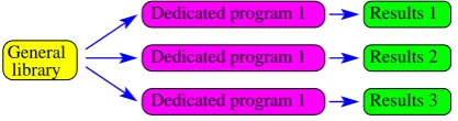
It is worth to mention that the computational implementa-tion with minimal coordinates is dramatically different from the one classically found with other coordinates. As illus-trated in Fig. 2, a multibody simulation software classically consists of a main general solver able to simulate various me-chanical systems, each of them being described in a specific data file. With minimal coordinates (Fig. 3), each application actually leads to a dedicated program, which is constructed

Dedicated program 1

General

library Dedicated program 1

Dedicated program 1

Results 1

Results 2

Results 3

Figure 3. Computational organization with minimal coordinates.

with the help of a multibody library. The latter is expected to provide routines which facilitate the expression of kine-matics and forces, and the construction and integration of the equations of motion.

When working with minimal coordinates, the equations of motion generally derive from the application of the d’Alembert’s principle. If the system comprises nB bodies

and ncp degrees of freedom, the ncp differential equations

governing the dynamic behaviour of the mechanical system are built according to

nB X

i=1

h

di,j·(Ri−miai)+θi,j·(MGi−ΦGiω˙i−ωi×ΦGiωi) i

=0

j=1,...,ncp (3)

with

– mi andΦGi the mass and the central inertia tensor of

body i;

– Riand MGithe resultant force and moment, at the centre

of gravity Gi, of all applied forces exerted on body i;

– aithe acceleration of the centre of gravity of body i;

– di,j_and_θi,j_{the partial contributions of ˙q}

jin the velocity

of the centre of gravity viand the rotational velocityωi

of body i, respectively, defined by

vi = ncp X

j=1

di,j·˙qj ↔ di,j= ∂vi ∂˙qj

(4)

ωi = ncp X

j=1

θi,j

·˙qj ↔ θi,j= ∂ωi ∂˙qj

. (5)

The resulting equations of motion have the classical fol-lowing form

M(q)·¨q+h(q,˙q)=g(q,˙q,t) (6) where, for example the mass matrix of dimension ncp×ncp,

is obtained by

Mjk= nB X

i=1

h

midi,j·di,k+θi,j·(ΦGi·θ

i,k₎i

(7)

while h represents the contribution of Coriolis, centrifugal and gyroscpic terms, and f the applied forces.

(5)

G. Kouroussis and O. Verlinden: Railway ground vibrations through multibody and FEM 171

0

x0 y0

z0

i

xi

yi

zi

T0,i

ei

Figure 4. Formalism of homogeneous transformation matrix.

– the kinematics of the system, that’s to say the expression of position, velocity, acceleration and partial velocities of each body i of the system in terms of the configura-tion parameters q and their first and second time deriva-tives;

– the applied efforts acting on each body i.

4.2.2 Kinematics

The expression of the complete kinematics, especially at ac-celeration level and for 3-D systems, is tricky, tedious and source of mistakes. To circumvent this difficulty, the Easy-Dynframework provides a symbolic script which automat-ically generates the expressions of velocities and accelera-tions from only the position information.

To express the kinematics at position level, the formalism of homogeneous transformation matrices was retained. The position and orientation of each body i is expressed by means of the homogeneous transformation matrix T0,igiving the

sit-uation of the local frame associated with body i with respect to the global reference frame 0 (Fig. 4). It is a 4×4 matrix of the following well-know form

T0,i=

R0,i {ei}i

0 0 0 1 !

(8)

where eiis the coordinate vector of frame i with respect to

the global coordinate system 0, and R0,iis the rotation tensor

describing the orientation of frame i with respect to frame 0. Practically, the homogeneous transformation matrices have the deciding advantage to enjoy the following property

Ti,k=Ti,j·Tj,k ∀i,j,k. (9)

This means that a complex motion can be elegantly de-fined as a succession of elementary motions (Fig. 5) like for example

T0,1=Trot. z(θ)·Tdisp(0,l,0) (10)

expressing a rotation about z of an angle θ followed by a displacement along the y-axis equal to l.

0

x0 y0

z0 i

xi yi

zi

j

xj yj

zj

T0,i T0,j

Ti,j

Telementary motion 1 Telementary motion 2 Telementary motion 3

. . .

0

i

Figure 5. Homogeneous transformation matrices: illustration of

the motion decomposition.

Translational and rotational velocities of each body i can then be easily obtained by differentiation of the homoge-neous transformation matrix giving its situation

{vi}0 =

d

dt{ei}0 (11)

{ω˜i}0 = R˙0,i·R T

0,i=

         

0 −ωz ωy

ωz 0 −ωx

−ω_y ω_x 0          

(12)

from which accelerations and partial velocities can be deter-mined by one more differentiation.

UnderEasyDyn, a symbolic script calledCAGeM, which stands for Computer-Aided generation of Motion, takes after the differentiation. The script can be run underMuPAD (Sci-Face Software GmbH & Co, 2012) or Xcas/Giac(Parisse and Graeve, 2010), the latter offering a completely open source environment.

4.2.3 Application to the vehicle modelling

In the present study, the vehicle is modelled by rigid bodies representing each inertial part of the train: car bodies, bo-gies, wheelsets and possibly wheel treads in case of compli-ant wheels (Kouroussis et al., 2012b), interconnected by the primary and secondary suspensions represented by springs and dampers.

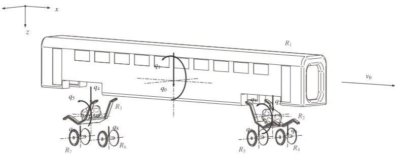
To illustrate the use of homogeneous transformation ma-trices, let us consider the carriage of Fig. 6. The motion of the car body R1 and bogies R2 and R3 is described by their

vertical displacements and their pitch angle, involving a total of 6 degrees of freedom q0to q5. The resulting homogeneous

transformation matrix of the first bogie R2is then written

T0,R2 = T disp_(v

0·t,0,q0)·Trot. y(q1)·Tdisp(lb/2,0,0)

·Trot. y(−q1)·Tdisp(0,0,q2)·Trot. y(q3) (13)

where Tdisp_(d

x,dy,dz) represents a translation and Trot. y(θ) a

(6)

x y

z

R1

R2

R3

R4

R5

R6

R7

v0

q0 q1

q2 q3 q5

q4

q6 q7

q8 q9

Figure 6.Vehicle modelling – kinematics in the xz-plane.

xxxxxxxxxxxxxxxxxxxxxxxxxxxxxxxxxxxxxxxxxxxxxxxxxxxxxxxxxxxxxxxxxxxxxxxxxxxxxxxxxxxxxxxxxxxxxxxxxxxxxxxxxxxxxxxxxxxxxxxxxxxxxxxxxxxxxxxxxxxxxxxxxxxxxxxxxxxxxxxxxxxxxxxxxxxxxxxxxxxxxxxxxxxxxxxxxxxxxxxxxxxxx xxxxxxxxxxxxxxxxxxxxxxxxxxxxxxxxxxxxxxxxxxxxxxxxxxxxxxxxxxxxxxxxxxxxxxxxxxxxxxxxxxxxxxxxxxxxxxxxxxxxxxxxxxxxxxxxxxxxxxxxxxxxxxxxxxxxxxxxxxxxxxxxxxxxxxxxxxxxxxxxxxxxxxxxxxxxxxxxxxxxxxxxxxxxxxxxxxxxxxxxxxxxx xxxxxxxxxxxxxxxxxxxxxxxxxxxxxxxxxxxxxxxxxxxxxxxxxxxxxxxxxxxxxxxxxxxxxxxxxxxxxxxxxxxxxxxxxxxxxxxxxxxxxxxxxxxxxxxxxxxxxxxxxxxxxxxxxxxxxxxxxxxxxxxxxxxxxxxxxxxxxxxxxxxxxxxxxxxxxxxxxxxxxxxxxxxxxxxxxxxxxxxxxxxxx xxxxxxxxxxxxxxxxxxxxxxxxxxxxxxxxxxxxxxxxxxxxxxxxxxxxxxxxxxxxxxxxxxxxxxxxxxxxxxxxxxxxxxxxxxxxxxxxxxxxxxxxxxxxxxxxxxxxxxxxxxxxxxxxxxxxxxxxxxxxxxxxxxxxxxxxxxxxxxxxxxxxxxxxxxxxxxxxxxxxxxxxxxxxxxxxxxxxxxxxxxxxx xxxxxxxxxxxxxxxxxxxxxxxxxxxxxxxxxxxxxxxxxxxxxxxxxxxxxxxxxxxxxxxxxxxxxxxxxxxxxxxxxxxxxxxxxxxxxxxxxxxxxxxxxxxxxxxxxxxxxxxxxxxxxxxxxxxxxxxxxxxxxxxxxxxxxxxxxxxxxxxxxxxxxxxxxxxxxxxxxxxxxxxxxxxxxxxxxxxxxxxxxxxxx xxxxxxxxxxxxxxxxxxxxxxxxxxxxxxxxxxxxxxxxxxxxxxxxxxxxxxxxxxxxxxxxxxxxxxxxxxxxxxxxxxxxxxxxxxxxxxxxxxxxxxxxxxxxxxxxxxxxxxxxxxxxxxxxxxxxxxxxxxxxxxxxxxxxxxxxxxxxxxxxxxxxxxxxxxxxxxxxxxxxxxxxxxxxxxxxxxxxxxxxxxxxx xxxxxxxxxxxxxxxxxxxxxxxxxxxxxxxxxxxxxxxxxxxxxxxxxxxxxxxxxxxxxxxxxxxxxxxxxxxxxxxxxxxxxxxxxxxxxxxxxxxxxxxxxxxxxxxxxxxxxxxxxxxxxxxxxxxxxxxxxxxxxxxxxxxxxxxxxxxxxxxxxxxxxxxxxxxxxxxxxxxxxxxxxxxxxxxxxxxxxxxxxxxxx xxxxxxxxxxxxxxxxxxxxxxxxxxxxxxxxxxxxxxxxxxxxxxxxxxxxxxxxxxxxxxxxxxxxxxxxxxxxxxxxxxxxxxxxxxxxxxxxxxxxxxxxxxxxxxxxxxxxxxxxxxxxxxxxxxxxxxxxxxxxxxxxxxxxxxxxxxxxxxxxxxxxxxxxxxxxxxxxxxxxxxxxxxxxxxxxxxxxxxxxxxxxx

subgrade (CLM model)

v0 x

z

m kp

kb dp

db

d

(Er,Ir,Ar,ρr)

Figure 7. The vehicle/track/foundation model.

The following observations can be made

– the global progression of the vehicle is assured by the

x coordinate of the form v0·t with v0the velocity and t the time;

– in this example, q3 is desired to strictly correspond to

the vertical relative displacement; that is why a back-ward rotation−q1 is imposed between the car and the bogie to compensate the pitch angle q1of the carbody.

On the other hand, the motion of wheelsets R4to R7comes

down to only the bounce motion, with respect to the bogie. For instance, the transformation matrix giving the situation of wheelset R7reads

T0,R7=T0,R2·T disp₍₋_l

w/2,0,0)·Trot. y(−q3)·Tdisp(0,0,q7) (14)

where lb and lwrepresent the distances between bogies and

wheelsets, respectively.

The formulation is not restrictive, and can be applied with-out any difficulty to more complex models and/or to three-dimensional kinematics.

4.2.4 Applied forces

The applied forces derive from gravity, suspensions and con-tact forces. The suspensions are classically defined as springs and dampers attached to specific points of the bodies. In the same manner, the contact forces are applied on the wheels. Their computation is explained further.

4.3 The track model

The track is represented by a finite element planar model, made up of 3 layers: the rail, the sleepers and the subgrade or foundation (Fig. 7). So far, only the vertical motion has been considered since the major contribution of ground vi-bration is induced by the vertical track deflection. Moreover, as symmetry is assumed, the track is condensed in the sym-metry plane and embraces the 2 rails. The reduced central rail (Young modulus Er, densityρr, geometrical moment of

inertia Ir and section Ar for a single rail) consists of a

suc-cession of Euler beams, while the sleepers correspond to lumped masses of mass m, placed with a regular spacing L. The sleepers are connected by spring-damper systems to the rail (stiffness kp and damping dp representing a single

rail-pad) and to the foundation (stiffness kband damping db

(7)

G. Kouroussis and O. Verlinden: Railway Ground Vibrations through Multibody and FEM 7

v0 x z m kp kb dp db d

(Er, Ir, Ar,ρr)

Figure 7.The vehicle/track/foundation model

xxxxxxxxxxxxxxxxxxxxxxxxxxxxxxxxxxxxxxxxxxxxxxxxxxxxxxxxxxxxxxxxxxxxxxxxxxxxxxxxxxxxxxxxxxxxxxxxxxxxxxxxxxxxxxxxxxxxxxxxxxxxxxxxxxxxxxxxxxxxxxxxxxxxxxxxxxxxxxxxxxxxxxxxxxxxxxxxxxxxxxxxxxxxxxxxxxxxxxxxxxxxxxxxxxxxxxxxxxxxxxxxxx xxxxxxxxxxxxxxxxxxxxxxxxxxxxxxxxxxxxxxxxxxxxxxxxxxxxxxxxxxxxxxxxxxxxxxxxxxxxxxxxxxxxxxxxxxxxxxxxxxxxxxxxxxxxxxxxxxxxxxxxxxxxxxxxxxxxxxxxxxxxxxxxxxxxxxxxxxxxxxxxxxxxxxxxxxxxxxxxxxxxxxxxxxxxxxxxxxxxxxxxxxxxxxxxxxxxxxxxxxxxxxxxxx xxxxxxxxxxxxxxxxxxxxxxxxxxxxxxxxxxxxxxxxxxxxxxxxxxxxxxxxxxxxxxxxxxxxxxxxxxxxxxxxxxxxxxxxxxxxxxxxxxxxxxxxxxxxxxxxxxxxxxxxxxxxxxxxxxxxxxxxxxxxxxxxxxxxxxxxxxxxxxxxxxxxxxxxxxxxxxxxxxxxxxxxxxxxxxxxxxxxxxxxxxxxxxxxxxxxxxxxxxxxxxxxxx xxxxxxxxxxxxxxxxxxxxxxxxxxxxxxxxxxxxxxxxxxxxxxxxxxxxxxxxxxxxxxxxxxxxxxxxxxxxxxxxxxxxxxxxxxxxxxxxxxxxxxxxxxxxxxxxxxxxxxxxxxxxxxxxxxxxxxxxxxxxxxxxxxxxxxxxxxxxxxxxxxxxxxxxxxxxxxxxxxxxxxxxxxxxxxxxxxxxxxxxxxxxxxxxxxxxxxxxxxxxxxxxxx xxxxxxxxxxxxxxxxxxxxxxxxxxxxxxxxxxxxxxxxxxxxxxxxxxxxxxxxxxxxxxxxxxxxxxxxxxxxxxxxxxxxxxxxxxxxxxxxxxxxxxxxxxxxxxxxxxxxxxxxxxxxxxxxxxxxxxxxxxxxxxxxxxxxxxxxxxxxxxxxxxxxxxxxxxxxxxxxxxxxxxxxxxxxxxxxxxxxxxxxxxxxxxxxxxxxxxxxxxxxxxxxxx xxxxxxxxxxxxxxxxxxxxxxxxxxxxxxxxxxxxxxxxxxxxxxxxxxxxxxxxxxxxxxxxxxxxxxxxxxxxxxxxxxxxxxxxxxxxxxxxxxxxxxxxxxxxxxxxxxxxxxxxxxxxxxxxxxxxxxxxxxxxxxxxxxxxxxxxxxxxxxxxxxxxxxxxxxxxxxxxxxxxxxxxxxxxxxxxxxxxxxxxxxxxxxxxxxxxxxxxxxxxxxxxxx xxxxxxxxxxxxxxxxxxxxxxxxxxxxxxxxxxxxxxxxxxxxxxxxxxxxxxxxxxxxxxxxxxxxxxxxxxxxxxxxxxxxxxxxxxxxxxxxxxxxxxxxxxxxxxxxxxxxxxxxxxxxxxxxxxxxxxxxxxxxxxxxxxxxxxxxxxxxxxxxxxxxxxxxxxxxxxxxxxxxxxxxxxxxxxxxxxxxxxxxxxxxxxxxxxxxxxxxxxxxxxxxxx xxxxxxxxxxxxxxxxxxxxxxxxxxxxxxxxxxxxxxxxxxxxxxxxxxxxxxxxxxxxxxxxxxxxxxxxxxxxxxxxxxxxxxxxxxxxxxxxxxxxxxxxxxxxxxxxxxxxxxxxxxxxxxxxxxxxxxxxxxxxxxxxxxxxxxxxxxxxxxxxxxxxxxxxxxxxxxxxxxxxxxxxxxxxxxxxxxxxxxxxxxxxxxxxxxxxxxxxxxxxxxxxxx xxxxxxxxxxxxxxxxxxxxxxxxxxxxxxxxxxxxxxxxxxxxxxxxxxxxxxxxxxxxxxxxxxxxxxxxxxxxxxxxxxxxxxxxxxxxxxxxxxxxxxxxxxxxxxxxxxxxxxxxxxxxxxxxxxxxxxxxxxxxxxxxxxxxxxxxxxxxxxxxxxxxxxxxxxxxxxxxxxxxxxxxxxxxxxxxxxxxxxxxxxxxxxxxxxxxxxxxxxxxxxxxxx xxxxxxxxxxxxxxxxxxxxxxxxxxxxxxxxxxxxxxxxxxxxxxxxxxxxxxxxxxxxxxxxxxxxxxxxxxxxxxxxxxxxxxxxxxxxxxxxxxxxxxxxxxxxxxxxxxxxxxxxxxxxxxxxxxxxxxxxxxxxxxxxxxxxxxxxxxxxxxxxxxxxxxxxxxxxxxxxxxxxxxxxxxxxxxxxxxxxxxxxxxxxxxxxxxxxxxxxxxxxxxxxxx xxxxxxxxxxxxxxxxxxxxxxxxxxxxxxxxxxxxxxxxxxxxxxxxxxxxxxxxxxxxxxxxxxxxxxxxxxxxxxxxxxxxxxxxxxxxxxxxxxxxxxxxxxxxxxxxxxxxxxxxxxxxxxxxxxxxxxxxxxxxxxxxxxxxxxxxxxxxxxxxxxxxxxxxxxxxxxxxxxxxxxxxxxxxxxxxxxxxxxxxxxxxxxxxxxxxxxxxxxxxxxxxxx kf kf kf

(a) Winkler model

xxxxxxxxxxxxxxxxxxxxxxxxxxxxxxxxxxxxxxxxxxxxxxxxxxxxxxxxxxxxxxxxxxxxxxxxxxxxxxxxxxxxxxxxxxxxxxxxxxxxxxxxxxxxxxxxxxxxxxxxxxxxxxxxxxxxxxxxxxxxxxxxxxxxxxxxxxxxxxxxxxxxxxxxxxxxxxxxxxxxxxxxxxxxxxxxxxxxxxxxxxxxxxxxxxxxxxxxxxxxxxxxxx xxxxxxxxxxxxxxxxxxxxxxxxxxxxxxxxxxxxxxxxxxxxxxxxxxxxxxxxxxxxxxxxxxxxxxxxxxxxxxxxxxxxxxxxxxxxxxxxxxxxxxxxxxxxxxxxxxxxxxxxxxxxxxxxxxxxxxxxxxxxxxxxxxxxxxxxxxxxxxxxxxxxxxxxxxxxxxxxxxxxxxxxxxxxxxxxxxxxxxxxxxxxxxxxxxxxxxxxxxxxxxxxxx xxxxxxxxxxxxxxxxxxxxxxxxxxxxxxxxxxxxxxxxxxxxxxxxxxxxxxxxxxxxxxxxxxxxxxxxxxxxxxxxxxxxxxxxxxxxxxxxxxxxxxxxxxxxxxxxxxxxxxxxxxxxxxxxxxxxxxxxxxxxxxxxxxxxxxxxxxxxxxxxxxxxxxxxxxxxxxxxxxxxxxxxxxxxxxxxxxxxxxxxxxxxxxxxxxxxxxxxxxxxxxxxxx xxxxxxxxxxxxxxxxxxxxxxxxxxxxxxxxxxxxxxxxxxxxxxxxxxxxxxxxxxxxxxxxxxxxxxxxxxxxxxxxxxxxxxxxxxxxxxxxxxxxxxxxxxxxxxxxxxxxxxxxxxxxxxxxxxxxxxxxxxxxxxxxxxxxxxxxxxxxxxxxxxxxxxxxxxxxxxxxxxxxxxxxxxxxxxxxxxxxxxxxxxxxxxxxxxxxxxxxxxxxxxxxxx xxxxxxxxxxxxxxxxxxxxxxxxxxxxxxxxxxxxxxxxxxxxxxxxxxxxxxxxxxxxxxxxxxxxxxxxxxxxxxxxxxxxxxxxxxxxxxxxxxxxxxxxxxxxxxxxxxxxxxxxxxxxxxxxxxxxxxxxxxxxxxxxxxxxxxxxxxxxxxxxxxxxxxxxxxxxxxxxxxxxxxxxxxxxxxxxxxxxxxxxxxxxxxxxxxxxxxxxxxxxxxxxxx xxxxxxxxxxxxxxxxxxxxxxxxxxxxxxxxxxxxxxxxxxxxxxxxxxxxxxxxxxxxxxxxxxxxxxxxxxxxxxxxxxxxxxxxxxxxxxxxxxxxxxxxxxxxxxxxxxxxxxxxxxxxxxxxxxxxxxxxxxxxxxxxxxxxxxxxxxxxxxxxxxxxxxxxxxxxxxxxxxxxxxxxxxxxxxxxxxxxxxxxxxxxxxxxxxxxxxxxxxxxxxxxxx xxxxxxxxxxxxxxxxxxxxxxxxxxxxxxxxxxxxxxxxxxxxxxxxxxxxxxxxxxxxxxxxxxxxxxxxxxxxxxxxxxxxxxxxxxxxxxxxxxxxxxxxxxxxxxxxxxxxxxxxxxxxxxxxxxxxxxxxxxxxxxxxxxxxxxxxxxxxxxxxxxxxxxxxxxxxxxxxxxxxxxxxxxxxxxxxxxxxxxxxxxxxxxxxxxxxxxxxxxxxxxxxxx xxxxxxxxxxxxxxxxxxxxxxxxxxxxxxxxxxxxxxxxxxxxxxxxxxxxxxxxxxxxxxxxxxxxxxxxxxxxxxxxxxxxxxxxxxxxxxxxxxxxxxxxxxxxxxxxxxxxxxxxxxxxxxxxxxxxxxxxxxxxxxxxxxxxxxxxxxxxxxxxxxxxxxxxxxxxxxxxxxxxxxxxxxxxxxxxxxxxxxxxxxxxxxxxxxxxxxxxxxxxxxxxxx xxxxxxxxxxxxxxxxxxxxxxxxxxxxxxxxxxxxxxxxxxxxxxxxxxxxxxxxxxxxxxxxxxxxxxxxxxxxxxxxxxxxxxxxxxxxxxxxxxxxxxxxxxxxxxxxxxxxxxxxxxxxxxxxxxxxxxxxxxxxxxxxxxxxxxxxxxxxxxxxxxxxxxxxxxxxxxxxxxxxxxxxxxxxxxxxxxxxxxxxxxxxxxxxxxxxxxxxxxxxxxxxxx xxxxxxxxxxxxxxxxxxxxxxxxxxxxxxxxxxxxxxxxxxxxxxxxxxxxxxxxxxxxxxxxxxxxxxxxxxxxxxxxxxxxxxxxxxxxxxxxxxxxxxxxxxxxxxxxxxxxxxxxxxxxxxxxxxxxxxxxxxxxxxxxxxxxxxxxxxxxxxxxxxxxxxxxxxxxxxxxxxxxxxxxxxxxxxxxxxxxxxxxxxxxxxxxxxxxxxxxxxxxxxxxxx xxxxxxxxxxxxxxxxxxxxxxxxxxxxxxxxxxxxxxxxxxxxxxxxxxxxxxxxxxxxxxxxxxxxxxxxxxxxxxxxxxxxxxxxxxxxxxxxxxxxxxxxxxxxxxxxxxxxxxxxxxxxxxxxxxxxxxxxxxxxxxxxxxxxxxxxxxxxxxxxxxxxxxxxxxxxxxxxxxxxxxxxxxxxxxxxxxxxxxxxxxxxxxxxxxxxxxxxxxxxxxxxxx

mf mf mf

df df df

kf kf kf

dc dc

kc kc

(b) CLM model

Figure 8. Foundation models (each discrete element is connected

to each sleeper)

rail above a sleeper and the vertical force applied at the same point. Indirect receptances correspond to rail displacement above the adjacent sleeper.

It appears that the CLM model properly captures the track receptances between 0Hz and 100Hz, which is not the case of the Winkler foundation. A good agreement can be ob-served between the CLM and the reference case: the error re-mains below 1dB which is well below the uncertainty range encountered in experimental receptances. The interest of this approach is certainly its ability to faithfully reproduce the track response with a limited number of degrees of freedom. The size of the model depends on the track length required to get the requested level of accuracy, that’s to say between 20 and 80 meters (Kouroussis et al., 2010). Practically, this represents the flexible part of the track, surrounded by rigid parts, with a transition area along which the compliance pro-gressively evolves. This assures a smooth loading of the soil and permits to manage vehicles longer than the considered track.

Concerning the degrees of freedom, the beam nodes

intro-0 20 40 60 80 100

−170 −165 −160 −155 −150

Frequency [Hz]

Amplitude [dB ref. 1 m/N] with a Winkler foundation

with a CLM foundation system layered soil

(a) Direct receptance

0 20 40 60 80 100

−170 −165 −160 −155 −150

Frequency [Hz]

Amplitude [dB ref. 1 m/N] with a Winkler foundation_{with a CLM foundation system}

layered soil

(b) Indirect receptance

Figure 9.Track receptances of the studied site (M´evernies —

Bel-gium)

duce 2 degrees of freedom (vertical displacement and slope) while each lumped mass, representing either a sleeper or a foundation mass, introduces one degree of freedom. Know-ing that 2 beam elements are defined between the sleepers, this leads, roughly speaking, to 6 degrees of freedom per sleeper, and consequently a few hundreds degrees of

free-www.mech-sci.net Mech. Sci.

to each sleeper).

As indicated in the state of the art, the model retained to represent the track is the CLM (coupled lumped mass) model proposed in Kouroussis et al. (2011a,b). It permits to prop-erly capture the track receptance even in presence of soft soils and therefore minimizes the error resulting from the hy-pothesis of track/soil decoupling. Compared to models based on the classical Winkler foundation representing one spring under each sleeper (Fig. 8a), it includes a better representa-tion of the soil under the track through a layer of lumped masses of mass mf placed below the sleepers (Fig. 8b), and

viscoelastically connected to the bedrock (stiffness kf and

the damping df) and to the surrounding foundation masses

(damping dcand stiffness kc). The values of the parameters

of the CLM model (mf, kf, df, kc, dc) are calculated, through

simple analytical relations (Kouroussis et al., 2011b), so as to match soil impedances issued from the FEM model of the soil1.

Figure 9 illustrates the accuracy of the CLM approach, by comparing the track receptances of a specific high-speed track in Belgium, lying on various foundation models, for the 3 following cases

– the track model is included in the three-dimensional FEM model of the soil, which can be considered as the reference solution;

– the proposed track model with a foundation represented by a Winkler foundation;

– the proposed track model where the CLM model is used for the foundation.

Presented direct receptances are defined as frequency re-sponse functions between the vertical displacement of the rail above a sleeper and the vertical force applied at the same

1_{Impedances issued from experimental tests or from other}

mod-els could be used equivalently.

G. Kouroussis and O. Verlinden: Railway Ground Vibrations through Multibody and FEM 7

v0 x z m kp kb dp db d

(Er, Ir, Ar,ρr)

Figure 7.The vehicle/track/foundation model

xxxxxxxxxxxxxxxxxxxxxxxxxxxxxxxxxxxxxxxxxxxxxxxxxxxxxxxxxxxxxxxxxxxxxxxxxxxxxxxxxxxxxxxxxxxxxxxxxxxxxxxxxxxxxxxxxxxxxxxxxxxxxxxxxxxxxxxxxxxxxxxxxxxxxxxxxxxxxxxxxxxxxxxxxxxxxxxxxxxxxxxxxxxxxxxxxxxxxxxxxxxxxxxxxxxxxxxxxxxxxxxxxx xxxxxxxxxxxxxxxxxxxxxxxxxxxxxxxxxxxxxxxxxxxxxxxxxxxxxxxxxxxxxxxxxxxxxxxxxxxxxxxxxxxxxxxxxxxxxxxxxxxxxxxxxxxxxxxxxxxxxxxxxxxxxxxxxxxxxxxxxxxxxxxxxxxxxxxxxxxxxxxxxxxxxxxxxxxxxxxxxxxxxxxxxxxxxxxxxxxxxxxxxxxxxxxxxxxxxxxxxxxxxxxxxx xxxxxxxxxxxxxxxxxxxxxxxxxxxxxxxxxxxxxxxxxxxxxxxxxxxxxxxxxxxxxxxxxxxxxxxxxxxxxxxxxxxxxxxxxxxxxxxxxxxxxxxxxxxxxxxxxxxxxxxxxxxxxxxxxxxxxxxxxxxxxxxxxxxxxxxxxxxxxxxxxxxxxxxxxxxxxxxxxxxxxxxxxxxxxxxxxxxxxxxxxxxxxxxxxxxxxxxxxxxxxxxxxx xxxxxxxxxxxxxxxxxxxxxxxxxxxxxxxxxxxxxxxxxxxxxxxxxxxxxxxxxxxxxxxxxxxxxxxxxxxxxxxxxxxxxxxxxxxxxxxxxxxxxxxxxxxxxxxxxxxxxxxxxxxxxxxxxxxxxxxxxxxxxxxxxxxxxxxxxxxxxxxxxxxxxxxxxxxxxxxxxxxxxxxxxxxxxxxxxxxxxxxxxxxxxxxxxxxxxxxxxxxxxxxxxx xxxxxxxxxxxxxxxxxxxxxxxxxxxxxxxxxxxxxxxxxxxxxxxxxxxxxxxxxxxxxxxxxxxxxxxxxxxxxxxxxxxxxxxxxxxxxxxxxxxxxxxxxxxxxxxxxxxxxxxxxxxxxxxxxxxxxxxxxxxxxxxxxxxxxxxxxxxxxxxxxxxxxxxxxxxxxxxxxxxxxxxxxxxxxxxxxxxxxxxxxxxxxxxxxxxxxxxxxxxxxxxxxx xxxxxxxxxxxxxxxxxxxxxxxxxxxxxxxxxxxxxxxxxxxxxxxxxxxxxxxxxxxxxxxxxxxxxxxxxxxxxxxxxxxxxxxxxxxxxxxxxxxxxxxxxxxxxxxxxxxxxxxxxxxxxxxxxxxxxxxxxxxxxxxxxxxxxxxxxxxxxxxxxxxxxxxxxxxxxxxxxxxxxxxxxxxxxxxxxxxxxxxxxxxxxxxxxxxxxxxxxxxxxxxxxx xxxxxxxxxxxxxxxxxxxxxxxxxxxxxxxxxxxxxxxxxxxxxxxxxxxxxxxxxxxxxxxxxxxxxxxxxxxxxxxxxxxxxxxxxxxxxxxxxxxxxxxxxxxxxxxxxxxxxxxxxxxxxxxxxxxxxxxxxxxxxxxxxxxxxxxxxxxxxxxxxxxxxxxxxxxxxxxxxxxxxxxxxxxxxxxxxxxxxxxxxxxxxxxxxxxxxxxxxxxxxxxxxx xxxxxxxxxxxxxxxxxxxxxxxxxxxxxxxxxxxxxxxxxxxxxxxxxxxxxxxxxxxxxxxxxxxxxxxxxxxxxxxxxxxxxxxxxxxxxxxxxxxxxxxxxxxxxxxxxxxxxxxxxxxxxxxxxxxxxxxxxxxxxxxxxxxxxxxxxxxxxxxxxxxxxxxxxxxxxxxxxxxxxxxxxxxxxxxxxxxxxxxxxxxxxxxxxxxxxxxxxxxxxxxxxx xxxxxxxxxxxxxxxxxxxxxxxxxxxxxxxxxxxxxxxxxxxxxxxxxxxxxxxxxxxxxxxxxxxxxxxxxxxxxxxxxxxxxxxxxxxxxxxxxxxxxxxxxxxxxxxxxxxxxxxxxxxxxxxxxxxxxxxxxxxxxxxxxxxxxxxxxxxxxxxxxxxxxxxxxxxxxxxxxxxxxxxxxxxxxxxxxxxxxxxxxxxxxxxxxxxxxxxxxxxxxxxxxx xxxxxxxxxxxxxxxxxxxxxxxxxxxxxxxxxxxxxxxxxxxxxxxxxxxxxxxxxxxxxxxxxxxxxxxxxxxxxxxxxxxxxxxxxxxxxxxxxxxxxxxxxxxxxxxxxxxxxxxxxxxxxxxxxxxxxxxxxxxxxxxxxxxxxxxxxxxxxxxxxxxxxxxxxxxxxxxxxxxxxxxxxxxxxxxxxxxxxxxxxxxxxxxxxxxxxxxxxxxxxxxxxx xxxxxxxxxxxxxxxxxxxxxxxxxxxxxxxxxxxxxxxxxxxxxxxxxxxxxxxxxxxxxxxxxxxxxxxxxxxxxxxxxxxxxxxxxxxxxxxxxxxxxxxxxxxxxxxxxxxxxxxxxxxxxxxxxxxxxxxxxxxxxxxxxxxxxxxxxxxxxxxxxxxxxxxxxxxxxxxxxxxxxxxxxxxxxxxxxxxxxxxxxxxxxxxxxxxxxxxxxxxxxxxxxx kf kf kf

(a) Winkler model

xxxxxxxxxxxxxxxxxxxxxxxxxxxxxxxxxxxxxxxxxxxxxxxxxxxxxxxxxxxxxxxxxxxxxxxxxxxxxxxxxxxxxxxxxxxxxxxxxxxxxxxxxxxxxxxxxxxxxxxxxxxxxxxxxxxxxxxxxxxxxxxxxxxxxxxxxxxxxxxxxxxxxxxxxxxxxxxxxxxxxxxxxxxxxxxxxxxxxxxxxxxxxxxxxxxxxxxxxxxxxxxxxx xxxxxxxxxxxxxxxxxxxxxxxxxxxxxxxxxxxxxxxxxxxxxxxxxxxxxxxxxxxxxxxxxxxxxxxxxxxxxxxxxxxxxxxxxxxxxxxxxxxxxxxxxxxxxxxxxxxxxxxxxxxxxxxxxxxxxxxxxxxxxxxxxxxxxxxxxxxxxxxxxxxxxxxxxxxxxxxxxxxxxxxxxxxxxxxxxxxxxxxxxxxxxxxxxxxxxxxxxxxxxxxxxx xxxxxxxxxxxxxxxxxxxxxxxxxxxxxxxxxxxxxxxxxxxxxxxxxxxxxxxxxxxxxxxxxxxxxxxxxxxxxxxxxxxxxxxxxxxxxxxxxxxxxxxxxxxxxxxxxxxxxxxxxxxxxxxxxxxxxxxxxxxxxxxxxxxxxxxxxxxxxxxxxxxxxxxxxxxxxxxxxxxxxxxxxxxxxxxxxxxxxxxxxxxxxxxxxxxxxxxxxxxxxxxxxx xxxxxxxxxxxxxxxxxxxxxxxxxxxxxxxxxxxxxxxxxxxxxxxxxxxxxxxxxxxxxxxxxxxxxxxxxxxxxxxxxxxxxxxxxxxxxxxxxxxxxxxxxxxxxxxxxxxxxxxxxxxxxxxxxxxxxxxxxxxxxxxxxxxxxxxxxxxxxxxxxxxxxxxxxxxxxxxxxxxxxxxxxxxxxxxxxxxxxxxxxxxxxxxxxxxxxxxxxxxxxxxxxx xxxxxxxxxxxxxxxxxxxxxxxxxxxxxxxxxxxxxxxxxxxxxxxxxxxxxxxxxxxxxxxxxxxxxxxxxxxxxxxxxxxxxxxxxxxxxxxxxxxxxxxxxxxxxxxxxxxxxxxxxxxxxxxxxxxxxxxxxxxxxxxxxxxxxxxxxxxxxxxxxxxxxxxxxxxxxxxxxxxxxxxxxxxxxxxxxxxxxxxxxxxxxxxxxxxxxxxxxxxxxxxxxx xxxxxxxxxxxxxxxxxxxxxxxxxxxxxxxxxxxxxxxxxxxxxxxxxxxxxxxxxxxxxxxxxxxxxxxxxxxxxxxxxxxxxxxxxxxxxxxxxxxxxxxxxxxxxxxxxxxxxxxxxxxxxxxxxxxxxxxxxxxxxxxxxxxxxxxxxxxxxxxxxxxxxxxxxxxxxxxxxxxxxxxxxxxxxxxxxxxxxxxxxxxxxxxxxxxxxxxxxxxxxxxxxx xxxxxxxxxxxxxxxxxxxxxxxxxxxxxxxxxxxxxxxxxxxxxxxxxxxxxxxxxxxxxxxxxxxxxxxxxxxxxxxxxxxxxxxxxxxxxxxxxxxxxxxxxxxxxxxxxxxxxxxxxxxxxxxxxxxxxxxxxxxxxxxxxxxxxxxxxxxxxxxxxxxxxxxxxxxxxxxxxxxxxxxxxxxxxxxxxxxxxxxxxxxxxxxxxxxxxxxxxxxxxxxxxx xxxxxxxxxxxxxxxxxxxxxxxxxxxxxxxxxxxxxxxxxxxxxxxxxxxxxxxxxxxxxxxxxxxxxxxxxxxxxxxxxxxxxxxxxxxxxxxxxxxxxxxxxxxxxxxxxxxxxxxxxxxxxxxxxxxxxxxxxxxxxxxxxxxxxxxxxxxxxxxxxxxxxxxxxxxxxxxxxxxxxxxxxxxxxxxxxxxxxxxxxxxxxxxxxxxxxxxxxxxxxxxxxx xxxxxxxxxxxxxxxxxxxxxxxxxxxxxxxxxxxxxxxxxxxxxxxxxxxxxxxxxxxxxxxxxxxxxxxxxxxxxxxxxxxxxxxxxxxxxxxxxxxxxxxxxxxxxxxxxxxxxxxxxxxxxxxxxxxxxxxxxxxxxxxxxxxxxxxxxxxxxxxxxxxxxxxxxxxxxxxxxxxxxxxxxxxxxxxxxxxxxxxxxxxxxxxxxxxxxxxxxxxxxxxxxx xxxxxxxxxxxxxxxxxxxxxxxxxxxxxxxxxxxxxxxxxxxxxxxxxxxxxxxxxxxxxxxxxxxxxxxxxxxxxxxxxxxxxxxxxxxxxxxxxxxxxxxxxxxxxxxxxxxxxxxxxxxxxxxxxxxxxxxxxxxxxxxxxxxxxxxxxxxxxxxxxxxxxxxxxxxxxxxxxxxxxxxxxxxxxxxxxxxxxxxxxxxxxxxxxxxxxxxxxxxxxxxxxx xxxxxxxxxxxxxxxxxxxxxxxxxxxxxxxxxxxxxxxxxxxxxxxxxxxxxxxxxxxxxxxxxxxxxxxxxxxxxxxxxxxxxxxxxxxxxxxxxxxxxxxxxxxxxxxxxxxxxxxxxxxxxxxxxxxxxxxxxxxxxxxxxxxxxxxxxxxxxxxxxxxxxxxxxxxxxxxxxxxxxxxxxxxxxxxxxxxxxxxxxxxxxxxxxxxxxxxxxxxxxxxxxx

mf _m_f _m_f

df df df

kf kf kf

dc dc

kc kc

(b) CLM model

to each sleeper)

rail above a sleeper and the vertical force applied at the same point. Indirect receptances correspond to rail displacement above the adjacent sleeper.

It appears that the CLM model properly captures the track receptances between 0Hz and 100Hz, which is not the case of the Winkler foundation. A good agreement can be ob-served between the CLM and the reference case: the error re-mains below 1dB which is well below the uncertainty range encountered in experimental receptances. The interest of this approach is certainly its ability to faithfully reproduce the track response with a limited number of degrees of freedom. The size of the model depends on the track length required to get the requested level of accuracy, that’s to say between 20 and 80 meters (Kouroussis et al., 2010). Practically, this represents the flexible part of the track, surrounded by rigid parts, with a transition area along which the compliance pro-gressively evolves. This assures a smooth loading of the soil and permits to manage vehicles longer than the considered track.

Concerning the degrees of freedom, the beam nodes

intro-0 20 40 60 80 100

−170 −165 −160 −155 −150

Frequency [Hz]

Amplitude [dB ref. 1 m/N] with a Winkler foundation_{with a CLM foundation system}

layered soil

(a) Direct receptance

0 20 40 60 80 100

−170 −165 −160 −155 −150

Frequency [Hz]

Amplitude [dB ref. 1 m/N] with a Winkler foundation

with a CLM foundation system layered soil

(b) Indirect receptance

Figure 9.Track receptances of the studied site (M´evernies —

Bel-gium)

duce 2 degrees of freedom (vertical displacement and slope) while each lumped mass, representing either a sleeper or a foundation mass, introduces one degree of freedom. Know-ing that 2 beam elements are defined between the sleepers, this leads, roughly speaking, to 6 degrees of freedom per sleeper, and consequently a few hundreds degrees of

free-www.mech-sci.net Mech. Sci.

Figure 9. Track receptances of the studied site (M´evernies –

Bel-gium).

point. Indirect receptances correspond to rail displacement above the adjacent sleeper.

(8)

this leads, roughly speaking, to 6 degrees of freedom per sleeper, and consequently a few hundreds degrees of freedom for the track.

5 Track interaction: wheel/rail contact forces

The contact forces between the wheels and the rail allow coupling between the vehicle and the track. We have chosen to calculate this force through the well-known Hertz contact theory, stating that the normal contact force N can be calcu-lated from the penetration d according to

N=KHzd3/2, (15)

where the coefficient KHzdepends only on the radii of

curva-ture of the wheel and the rail profiles, and the elastic proper-ties of the material of both bodies.

The penetration for each wheel i depends on the vehicle and track states and is calculated from

dwheel,i=zrail(xwheel,j)−zwheel,i+h(xwheel,i)+Rwheel,i (16)

with

– xwheel,iand zwheel,ithe coordinates of the centre of wheel

i, depending on the configuration parameters of the

ve-hicle;

– zrail(xwheel,j) the height of the rail below wheel i,

de-pending on the degrees of freedom of the track model, through the shape functions of the beam elements;

– Rwheel,ithe radius of wheel i;

– h(xwheel,i) the rail irregularity below wheel i, which can

consist of local defects and/or overall track contribution like roughness (Kouroussis et al., 2010).

The action and reaction components of the contact force can then be applied to the multibody and track models. Let us note that, for the track, the force is transformed to nodal forces and torques, again through the shape functions of the beam element, calculated at the contact point.

Let us note that most of ground vibration models consider a linear relationship between the contact force and the pen-etration, neglecting the inherent non-linearity of the contact physics.

Numerical framework

The track/vehicle model explained in the previous sections has been implemented as a C++program based on the home-madeEasyDynlibrary (Kouroussis et al., 2011c; Verlinden et al., 2013).

The equations of motion and of the vehicle (Eq. 1) and of the track (Eq. 2), are rewritten in the following residual form

f (q,˙q,¨q,t)=

(

Mv·q¨v+hv(qv,˙qv,t)−fv(qv,qt,t)

Mt·q¨t+Ct·˙qt+Kt·qt−ft(qv,qt,t)

) =0 (17)

where the global vector of configuration parameters q results from the concatenation of the vehicle and track configuration parameters

q=

(

qv qt

)

. (18)

When rewritten in this form, the equations can be inte-grated by the routines provided by thesim module, which implement the so-called Newmark-1/4 method. The latter is known to not introduce any numerical damping which is an advantage in the considered application. Numerical damping is anyway unnecessary as we deal with ordinary differential equations.

The vehicle is a multibody system and its equations of mo-tion are computed from the routines offered by thembs mod-ule. This assumes that the user provides two routines imple-menting on the one hand the kinematics of the multibody system and, on the other hand, the forces exerted on each body, corresponding in our case to the gravity, the suspen-sion forces and the contact forces. Let us recall that concern-ing the kinematics, the velocities, accelerations and partial velocities are generated symbolically by the scriptCAGeM

accompanying the C++library ofEasyDyn.

The equations of motion of the track (Eq. 2) are simple and are coded directly in C++ by using the classical assembly techniques.

The computer implementation is summarized in Fig. 10. Let us note that, thanks to thevisu module, shapes can be attached to bodies, in order to visualize the motion of the system.

6 Soil simulation

The simulation of the vehicle/track subsystem provides the time history of the ground forces, defined as the visco-elastic action of the ballast on the subgrade. These forces are used in the second subproblem, managed under the finite element softwareABAQUSwhich computes the free field response.

The finite element model of the soil is out of the scope of this paper, a detailed description of the finite element model being available in Kouroussis et al. (2010, 2012a). Let us mention anyway that

– only a half soil is considered due to the assumed left-right symmetry;

– the forces are not applied on nodes but on rigid surfaces corresponding to the area covered by the sleepers;

– the inner part of the model consists of one quarter of a sphere and defines the specific geometry of the consid-ered track;

(9)

100 010 110

simulation of the soil subsystem (under ABAQUS)

100 010 110

time domain evolution animation

visualization

*.res _*.vol

*.van Vehicle data

Equations of motion of the vehicle

EasyDyn libraries

link editor stiffness and mass

elementary matrices writing

rail equations of motion

differential equations of the vehicle/track/foundation subsystem wheel/rail

contact law stochastic generation

process of the rail unevenness Simulation parameters

initial conditions position and speed of the vehicle local defect

definition

contact location search (rail)

contact forces calculation sleepers equations

of motion rail forces (at

nodes)

numerical integration (Newmark) configuration parameters saving

ballast reaction saving

bodies position saving

bodies definition (shape) wheelset

reaction interpolation

polynomials definition initialisation (rail)

initialisation (contact) Track and foundation data

foundation equation of motion

Figure 10.Computer implementation of the vehicle/track model.

3.00 3.00

5.02 14.00 3.13

3.00

3.14 18.70

3.00

18.70

3.00 3.00

18.70 18.70

THALYS

Figure 11.Thalys HST dimensions

7 Example: the Thalys high-speed train

7.1 Description of the model

Thalys trains are designed to operate over the French, Bel-gian, German and Dutch networks and therefore ensure the interconnection between the different high-speed lines. The high-speed vehicle studied in this work stems from the same generation as the French TGV Atlantique with some

(10)

xxxxxxxxxxxxxxxx

x

z

v0

(a) Old model

xxxxxxxxxxxxxxxxxxxx

x

z

v0

(b) New model

Figure 12.Studied multibody models for the vehicle

Table 1.Dynamic parameters of Thalys HST — unladen weight

Bogie Bogie Bogie

Y230A Y237A Y237B

Carbody mass mc[kg] 26721 14250 20426

Carbody pitch moment of inertia Ic[×106kgm2] 1.15 0.61 0.88

Bogie mass mb[kg] 3261 15650 8156

Bogie pitch moment of inertia Ib[kgm2] 2870 13750 7185

Wheelset mass m0[kg] 2009 2050 2009

Primary suspension stiffness k1[MN/m] 2.09 1.63 2.09

Primary suspension damping d1[kNs/m] 40 40 40

Secondary suspension stiffness k2[MN/m] 2.45 0.93 2.45

Secondary suspension damping d2[kNs/m] 40 40 40

the side carriage bogies, which connect the power carriages (at the outer extremities of the train) to the main passen-ger carriages (in the centre of the train). The unladen mass is close to 386 tonnes, while the nominal loading is worth 439 tonnes.

Three bogie types are used in this vehicle:

– the Y230A motor bogie equipping the locomotives;

– the Y237 trailing bogie: variant A for the side carriages

and variant B for the other ones.

An SR 10 pneumatic air-sprung suspension is used as the sec-ondary suspension of the trailing bogies while the coil spring is preferred for the primary suspension. For the Y230A, clas-sical rubber sandwich block (coil) spring is used for the pri-mary (secondary) suspension. Table 1 summarizes the dy-namic parameters of the bogies in terms of mass, stiffness and damping.

The Thalys HST has already been studied by the au-thors (Kouroussis et al., 2011e). However, due to a lack in the vehicle data that we were able to collect, the pitch mo-tion of the bogie and carbodies was neglected. The bogie and the carbody were actually replaced by a front and a rear

lumped mass whose only bounce motion was taken into ac-count (Figure 12(a)). The present model consists of a succes-sion of carbodies, bogies and wheelsets involving 2 degrees of freedom (bounce and pitch) for each carbody/bogie and 1 degree of freedom (bounce) for each wheelset (Figure 12(b)). The Thalys HST, in its general configuration consists of a succession of one locomotive, one side carriage, six central carriages, one side carriage and finally one locomotive, with a total of 72 degrees of freedom. The relevant geometrical data of the train are specified in Table 2.

If the vehicle rides at velocity v0, the position matrices relative to the first locomotive are written

T0,carbody = Tdisp(v0t,0,ql,1)·Trot. y(ql,2) (19) T0,f ront bogie = Tdisp(v0t+lb/2,0,ql,3)·Trot. y(ql,4) (20) T0,rear bogie = Tdisp(v0t−lb/2,0,ql,5)·Trot. y(ql,6) (21)

T0,f irst wheel = Tdisp(v0t+lb/2+lw/2,0,ql,7) (22) T0,second wheel = Tdisp(v0t+lb/2−lw/2,0,ql,8) (23) T0,third wheel = Tdisp(v0t−lb/2+lw/2,0,ql,9) (24)

T0,f ourth wheel = Tdisp(v0t−lb/2−lw/2,0,ql,10) (25)

where ql,i are the 10 configuration parameters of the

loco-Mech. Sci. www.mech-sci.net

Figure 12. Studied multibody models for the vehicle.

Table 1.Dynamic parameters of Thalys HST – unladen weight.

Bogie Bogie Bogie

Y230A Y237A Y237B

Carbody mass mc[kg] 26 721 14 250 20 426

Carbody pitch moment of inertia Ic[×106_{kg m}2_] ₁_.₁₅ ₀_.₆₁ ₀_.₈₈

Bogie mass mb[kg] 3261 15 650 8156

Bogie pitch moment of inertia Ib[kg m2_] ₂₈₇₀ _{13 750} ₇₁₈₅

Wheelset mass m0[kg] 2009 2050 2009

Primary suspension stiffness k1[MN m−1_] ₂_.₀₉ ₁_.₆₃ ₂_.₀₉

Primary suspension damping d1[kNs m−1_] ₄₀ ₄₀ ₄₀

Secondary suspension stiffness k2[MN m−1_] ₂_.₄₅ ₀_.₉₃ ₂_.₄₅ Secondary suspension damping d2[kNs m−1_] ₄₀ ₄₀ ₄₀

the side carriage bogies, which connect the power carriages (at the outer extremities of the train) to the main passen-ger carriages (in the centre of the train). The unladen mass is close to 386 tonnes, while the nominal loading is worth 439 tonnes.

Three bogie types are used in this vehicle:

– the Y230A motor bogie equipping the locomotives; – the Y237 trailing bogie: variant A for the side carriages

and variant B for the other ones.

An SR 10 pneumatic air-sprung suspension is used as the sec-ondary suspension of the trailing bogies while the coil spring is preferred for the primary suspension. For the Y230A, clas-sical rubber sandwich block (coil) spring is used for the pri-mary (secondary) suspension. Table 1 summarizes the dy-namic parameters of the bogies in terms of mass, stiffness and damping.

The Thalys HST has already been studied by the au-thors (Kouroussis et al., 2011e). However, due to a lack in the vehicle data that we were able to collect, the pitch mo-tion of the bogie and carbodies was neglected. The bogie and the carbody were actually replaced by a front and a rear lumped mass whose only bounce motion was taken into

ac-count (Fig. 12a). The present model consists of a succession of carbodies, bogies and wheelsets involving 2 degrees of freedom (bounce and pitch) for each carbody/bogie and 1 degree of freedom (bounce) for each wheelset (Fig. 12b).

The Thalys HST, in its general configuration consists of a succession of one locomotive, one side carriage, six central carriages, one side carriage and finally one locomotive, with a total of 72 degrees of freedom. The relevant geometrical data of the train are specified in Table 2.

If the vehicle rides at velocity v0, the position matrices

rel-ative to the first locomotive are written

T0,carbody = Tdisp(v0t,0,ql,1)·Trot. y(ql,2) (19)

T0,front bogie = Tdisp(v0t+lb/2,0,ql,3)·Trot. y(ql,4) (20)

T0,rear bogie = Tdisp(v0t−lb/2,0,ql,5)·Trot. y(ql,6) (21)

T0,first wheel = Tdisp(v0t+lb/2+lw/2,0,ql,7) (22)

T0,second wheel = Tdisp(v0t+lb/2−lw/2,0,ql,8) (23)

T0,third wheel = Tdisp(v0t−lb/2+lw/2,0,ql,9) (24)

T0,fourth wheel = Tdisp(v0t−lb/2−lw/2,0,ql,10) (25)

where ql,i are the 10 configuration parameters of the

loco-motive, with ql,1 and ql,2 the bounce and pitch motions of

(11)

Table 2.Geometric parameters of Thalys HST.

Parameter Symbol Value (m)

Distance between bogies on locomotive lb 14

Bogie wheelbase lb 3

Distance between locomotive COM and side carriage COM dlb 23.12

Central carriage length b 18.7

Table 3.Studied site parameters (M´evernies – Belgium).

Track parameters

Er Ir ρr Ar d

210 GPa 3055 cm4 _{7850 kg m}−3 ₆₃_._{9 cm}2 ₀_._{6 m}

kp dp kb db m

120 MN m−1 _{4 kNs m}−1 _{47 MN m}−1 _{72 kNs m}−1 _{150 kg}

Soil parameters

layer d E ρ ν

1 2.7 m 129 MPa 1600 kg m−3 ₀_.₃

2 3.9 m 227 MPa 2000 kg m−3 ₀_.₃

3 ∞ 659 MPa 2000 kg m−3 ₀_.₃

mf kf df kc dc

460 kg 40 MN m−1 _{426 kNs m}−1 _{63 MN m}−1 ₋_{73 kNs m}−1

motions of the front (rear) bogie, and ql,7to ql,10 the bounce

motions of the wheelsets. For the side carriages, we get

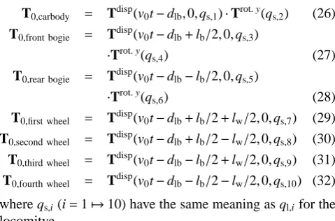
T0,carbody = Tdisp(v0t−dlb,0,qs,1)·Trot. y(qs,2) (26)

T0,front bogie = Tdisp(v0t−dlb+lb/2,0,qs,3)

·Trot. y(qs,4) (27)

T0,rear bogie = Tdisp(v0t−dlb−lb/2,0,qs,5)

·Trot. y(qs,6) (28)

T0,first wheel = Tdisp(v0t−dlb+lb/2+lw/2,0,qs,7) (29)

T0,second wheel = Tdisp(v0t−dlb+lb/2−lw/2,0,qs,8) (30)

T0,third wheel = Tdisp(v0t−dlb−lb/2+lw/2,0,qs,9) (31)

T0,fourth wheel = Tdisp(v0t−dlb−lb/2−lw/2,0,qs,10) (32)

where qs,i(i=17→10) have the same meaning as ql,ifor the

locomitve.

There is only one bogie per central carriage, which is the rear one, the front one being kinematically attached to the previous carriage. The corresponding position matrices of the

j-th central carriage then read

T0,carbody j = Tdisp(v0t−dlb−lb/2−(2 j−1)b/2,0,qc j,1)

·Trot. y(qc j,2) (33)

T0,rear bog.j = Tdisp(v0t−dlb−lb/2−jb,0,qc j,3)

·Trot. y(qc j,4) (34)

T0,1t wheel j = Tdisp(v0t−dlb−lb/2−jb+lw/2,0,qc j,5) (35)

T0,2nd wheel j = Tdisp(v0t−dlb−lb/2−jb−lw/2,0,qc j,6) (36)

with qc j,i(i=17→6 and j=17→6) the configuration

param-eters of the carriage, defined in the same manner as previ-ously.

The track model involves 160 sleepers. The parameters of the track and of the CLM model used to represent the foun-dation are pointed out in Table 3. The CLM parameters issue from the identification of the foundation receptance with re-spect to a 3-D FEM model of the soil comprising 3 layers. For each layer, the depth d, the Young modulus E, the den-sityρand the Poisson’s numberνare also given in Table 3. Let us note that the damping dcis negative, so as to properly

capture the ground wave propagation delay, also called “tau effect”.

7.2 Simulation results 7.2.1 Studied configurations

In the next sections, the results provided by three different models are compared

– The initial model Kouroussis et al. (2011e), without the pitch motion of bogies and carbodies and a Win-kler foundation for the track subgrade. It is denoted by model A.

(12)

-100 -50 0

Force [kN]

(a) Static axle load acting on the track

0 0.5 1 1.5 2 2.5 3

0 5

Time [s]

Differences [kN]

0 1 2 3

−100 −50 0

Time [s]

Force [kN]

Model A Model B Model C

(b) Ballast reaction used as input in the soil model

Figure 13.Time history of track/foundation forces for each model

In all cases, the train speed is worth v0=300km/h and the

rail irregularity is calculated for a rail quality of 6 (Garg and Dukkipati, 1984; Kouroussis et al., 2012a).

7.2.2 Forces on the track

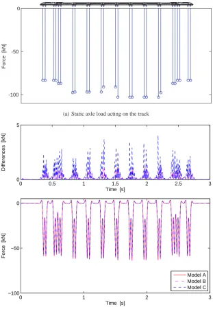
Figure 13(b) shows the time history of the force exerted by the track on the soil at the centre of the model, for each

model. In addition to these curves, the difference of force magnitudes provided by models B and C, compared to model A, is presented. This force, along with the ones under the other sleepers, is used as input in the FEM model of the soil to study the wave propagation. The plot is to compare with the one of Figure 13(a) which shows the static load on the track, in function of a pseudo-time corresponding to the dis-tance divided by the velocity. The figures show how the track

Mech. Sci. www.mech-sci.net

Figure 13. Time history of track/foundation forces for each model.

– The complete model, denoted by model C, as described in this paper with the CLM model and the pitch motion of bogies and carbodies.

In all cases, the train speed is worth v0=300 km h−1 and

the rail irregularity is calculated for a rail quality of 6 (Garg and Dukkipati, 1984; Kouroussis et al., 2012a).

7.2.2 Forces on the track

Figure 13b shows the time history of the force exerted by the track on the soil at the centre of the model, for each model. In addition to these curves, the difference of force magnitudes

provided by models B and C, compared to model A, is pre-sented. This force, along with the ones under the other sleep-ers, is used as input in the FEM model of the soil to study the wave propagation. The plot is to compare with the one of Fig. 13a which shows the static load on the track, in function of a pseudo-time corresponding to the distance divided by the velocity. The figures show how the track distributes the contact forces through the sleepers.

(13)

25 50 75 100

10−4 10−2 100 102

Frequency [Hz]

Force [kN]

Model A Model B Model C

fa

fa/2

fc

Figure 14. Frequency content of ballast reaction force for each model.

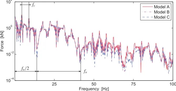
than 5 % between models A and C. This is confirmed by the corresponding frequency content, illustrated in Fig. 14. The latter reveals the usual peaks, related to the carriage pas-sage excitation mechanisms at frequency fc=v0/lb=4.5 Hz

modulated in amplitude by the fundamental axle passage fre-quency fa=v0/lw=27.8 Hz. The magnitudes at frequency

k

2fa(k=1,3,5,...) are completely suppressed.

The analysis shows that on one hand the benefit brought by the CLM model is not significant, due to the fact that the soil is relatively rigid. On the other hand, the differences observed with model C, although limited, indicate the importance of a careful vehicle modelling in the prediction of railway in-duced ground vibrations.

7.2.3 Ground vibrations

Figure 15 shows the time history of the vertical ground veloc-ity at 9 m from the track, resulting from the application of the ballast reaction forces, obtained from the simulation of each vehicle/track model, on the 3-D FEM model of the soil. The figure also includes the experimental results presented in a previous work (Kouroussis et al., 2011e). The corresponding weighted severity can be found in Fig. 16, as defined in the DIN 4150 part 2 standard (Deutsches Institut f¨ur Normung, 1999). This indicator provides a quantification of the maxi-mum vibratory dose felt by residents, and presents an inter-esting basis for drawing a parallel between discomfort and ground vibrations. Finally, Fig. 17 shows the frequency con-tent of the ground velocity and indicates the maximum am-plitude at 26 Hz. The latter is imposed by a resonance-like phenomenon, where the soil surface vibrates in phase with the vertical loading at a frequency corresponding to

flayer=cP

4d (37)

with cPthe compression wave velocity of the first layer and

d its depth.

The following observations are noteworthy:

– The comparison of the results obtained from models A, B and C leads to the same conclusions as in the previ-ous section. The difference between models A/B and C is clearly observed on the weighted severity, at the be-ginning and end of the ground vibration. In the same way, the frequency contents differ in mid and high fre-quencies. Note that the experimental values at 23 m have greater amplitude than those at 25 and 18 m, whose ori-gin is unfortunately unknown.

– Figures 15 and 16 show a good agreement between pre-dicted and experimental ground vibrations, which vali-dates the hypothesis made by the authors concerning the track/soil decoupling when the soil is sufficiently rigid with respect to the ballast (Kouroussis et al., 2012a). It must however be mentioned that the vibration peaks predicted in the frequency ranges 20–30 Hz and 50– 60 Hz (Fig. 17) are larger than their experimental coun-terparts. At high frequencies, the gap is explained by the adopted material damping in the soil model: a time do-main simulation imposes a viscous damping although the hysteretic damping better corroborates for soil mo-tion since it does not significantly depend on the fre-quency of motion.

As a final result, Fig. 18 shows how the the peak particle velocity PPV and the KBF,maxindicators evolve with the