A graph-theoretic approach to sparse matrix inversion for implicit differential algebraic equations

(1)

www.mech-sci.net/4/243/2013/ doi:10.5194/ms-4-243-2013

©Author(s) 2013. CC Attribution 3.0 License.

Mechanical

Sciences

Open Access

A graph-theoretic approach to sparse matrix inversion

for implicit differential algebraic equations

H. Yoshimura

Department of Applied Mechanics and Aerospace Engineering, Waseda University, Ohkubo, Shinjuku, Tokyo 169-8555, Japan

Correspondence to: H. Yoshimura ([email protected])

Received: 15 November 2012 – Revised: 9 March 2013 – Accepted: 5 April 2013 – Published: 6 June 2013

Abstract. In this paper, we propose an efficient numerical scheme to compute sparse matrix inversions for Implicit Differential Algebraic Equations of large-scale nonlinear mechanical systems. We first formulate me-chanical systems with constraints by Dirac structures and associated Lagrangian systems. Second, we show how to allocate input-output relations to the variables in kinematical and dynamical relations appearing in DAEs by introducing an oriented bipartite graph. Then, we also show that the matrix inversion of Jacobian matrix associated to the kinematical and dynamical relations can be carried out by using the input-output rela-tions and we explain solvability of the sparse Jacobian matrix inversion by using the bipartite graph. Finally, we propose an efficient symbolic generation algorithm to compute the sparse matrix inversion of the Jacobian matrix, and we demonstrate the validity in numerical efficiency by an example of the stanford manipulator.

1 Introduction

Multibody systems such as space structures, manipulators, etc. are known to be represented as implicit mechanical sys-tems with kinematical constraints, holonomic or nonholo-nomic, which may be eventually expressed by implicit non-linear Differential-Algebraic Equations (DAEs). In particu-lar, for the numerical integration of such DAEs, we need to employ stiffly stable implicit numerical integrators such as Backward Differentiation Formula (see, Hachtel et al., 1971; Brayton et al., 1972), since the DAEs are to be highly nonlin-ear and stiffin general. On the other hand, one may face at a serious problem in CPU time for solving the implicit nonlin-ear algebraic equations, especially, for the case of large-scale systems. Namely, increasing degrees of freedom of the sys-tem, it eventually requires much CPU time in computing the matrix inversion of Jacobian matrix of the implicit DAEs in Newton’s iteration at each time, since the Jacobian matrix of discretized nonlinear algebraic equations may be random sparse in general.

A major stumbling block lies in the fact that the Jacobian matrix has the random sparseness as well as highly nonlin-ear in terms of generalized coordinates. So far, some

nu-merical technique of sparse matrix inversions for VLSI cir-cuits or networks has been developed by using the block-triangularization of matrices (see, for instance, Orlandea et al., 1977a; Murata et al., 1985), where a structural analysis is effectively made by means of graph and matroid theory (for instance, refer to Murota, 2000). In these conventional approaches, one may properly find out pivots in the Gaus-sian elimination process at each time step in an ad hoc way (where we note that the choice of pivots is quite relevant with

input-output relations as will be shown shortly). This

eventu-ally requires much CPU time to calculate the inversion of the Jacobian matrix unless utilizing some effective sparse matrix algorithms. Namely, it is almost impossible to figure out a prior fill-in and fill-out in Gaussian elimination since

topo-logical structure of such a sparse Jacobian matrix might be

so much random and complicated. Thus, we need to develop an efficient numerical algorithm of sparse matrix inversion for solving large-scale implicit DAEs in a systematic way.

(2)

elements, in which systems are comprised of constitutive

re-lations of physical elements, structural rere-lations among the

physical relations, and causal (input-output) relations among physical variables. In particular, focusing upon the

input-output relations associated with all the kinematical and

dy-namical relations of original mechanical systems, we develop

bipartite graphs and then we show how the sparse matrix

inversion can be made by effectively using the input-output relations. Furthermore, we explain solvability for the sparse Jacobian matrix inversion associated to the DAEs by using the bipartite graph. Finally, we propose an efficient and sys-tematic symbolic generation algorithm to compute the sparse matrix inversion of the Jacobian matrix and we demonstrate its validity in numerical efficiency by an example of the stan-ford manipulator.

2 Implicit Lagrangian systems

Let us review Dirac structures and associated implicit

La-grangian systems by following Yoshimura and Marsden

(2006a,b, 2008).

2.1 Dirac structures

Let Qbe an n-dimensional configuration manifold, whose kinematical constraints are given by a constraint distribution ∆Q⊂TQ, given by, at each q∈ Q,

∆Q(q)={v∈TqQ | hωa(q),vi=0,a=1,...,m}, (1)

whereωa_{are m one-forms on}_Q_{. Define the distribution}_∆ T∗_Q on T∗_Q_by

∆T∗_Q=(Tπ_Q)−1(∆_Q)⊂T T∗Q,

where TπQ: T T∗Q →TQis the tangent map of the cotan-gent bundle projectionπQ: T∗Q → Q, while the annihilator of∆T∗_Qcan be defined by, for each z∈T∗

qQ,

∆◦

T∗_Q(z)={αz∈Tz∗T ∗_{Q | h}_α

z,wzi=0

for all wz∈∆T∗_Q(z)}.

LetΩbe the canonical symplectic structure on T∗_Q_and_Ω[_: T T∗_{Q →}_T∗_T∗_Q_{be the associated bundle map. Then, a Dirac} structure D_∆Qon T

∗_Q_{induced from}_∆

Qcan be defined by, for each z∈T∗

qQ,

D_∆Q(z)={(wz,αz)∈TzT ∗_{Q ×}_T∗

zT ∗_{Q |}

wz∈∆T∗_Q(z) and α_z−Ω[(z)·w_z∈∆◦ T∗_Q(z)}.

2.2 Local representations

Let us choose local coordinates qi_on_Q_{so that}_Q_{is locally} represented by an open set W⊂_Rn_{. The constraint set}_∆

Q defines a subspace of TQ, which we denote by∆(q)⊂_Rnat

each point q∈W. If the dimension of∆(q) is n−m, then we

can choose a basis em+1(q),em+2(q),...,en(q) of∆(q). Recall that the constraint sets can be also represented by the annihilator of∆(q), which is denoted by∆◦_{(q) spanned} by such one-forms that we write as ω1_,ω2_,...,ωm_{. Using}

πQ: T∗Q → Q locally denoted by z=(q,p)7→q and TπQ: T T∗_{Q →}_T_Q_{; (q}_,_p_,_˙q_,_˙p)_7→_(q_,_{˙q), it follows that}

∆T∗_Q{(q,p,˙q,˙p)|q∈U,˙q∈∆(q)}.

Let points in T∗_T∗_Q_{be locally denoted by (q}_,_p_,β,_{u), where}

βis a covector and u is a vector. Then, the annihilator of∆T∗_Q is locally represented as

∆◦

T∗_Q{(q,p,β,u)|q∈U, β∈∆

◦_{(q) and u}₌₀_}_.

Since we have the local formulaΩ[(q,p)·w(q,p)=(q,p,−˙p,˙q), the condition α(q,p)−Ω[(q,p)·w(q,p)∈∆◦_T∗_Q reads α+˙p∈ ∆◦_{(q), and w}₋_˙q₌_{0, where} _α

(q,p)=(q,p,α,w) and w(q,p)= (q,p,˙q,˙p). Thus, the induced Dirac structure is locally repre-sented by

D_∆Q(q,p)={(( ˙q,˙p),(α,w))|˙q∈∆(q),

w=˙q, α+˙p∈∆◦(q)}. (2) Representation (I): let us introduce a matrix representation

of D_∆Q given in Eq. (2). First, let N

T_{(q) be an n}_×_{m matrix}

whose m-column vectors ω1_(q)_,...,ωm_{(q) span the basis of} ∆◦_{(q), namely, N}T_(q)₌_[_ω1_(q)_,...,ωm_{(q)] and the distribution} ∆(q)⊂_RnTqQmay be represented by

∆(q)={˙q∈_Rn|N(q) ˙q=0}.

Using Lagrange multipliersλ=(λ1,...,λm)∈Rm, one has ∆◦

(q)=nβ∈(Rn)∗|β=NT(q)λ

o

.

Thus, the induced Dirac structure can be represented by

D_∆Q(q,p)={(( ˙q,˙p),(α,w))|N(q) ˙q=0,

w=˙q, α+˙p=NT(q)λo. (3)

Representation (II): as shown in Eq. (3), for

Representa-tion (I) for the induced Dirac structure, we utilized the La-grange multipliers, which represent constraint forces in con-strained mechanical systems. Here, we develop another rep-resentation of D_∆Q on T

∗_Q_{without using the Lagrange}

mul-tipliers.

Let us choose an n×(n−m) matrix B(q)=

[em+1(q),...,en(q)], whose column vectors span the basis of ∆(q). Then, it follows that the distribution∆(q)⊂_RnTqQ can be also represented by

∆(q)={˙q∈_Rn|˙q=B(q) u},

where u=(um+1,...,un)∈_Rn−m. Note that the orthogonality condition between N(q) and B(q) holds:

(3)

The above condition naturally comes from the fact that∆◦_is the annihilator of the distribution∆; namely, in other words, the basis em+1(q),...,en(q) is orthogonal to the dual basis

ω1_(q)_,...,ωm_{(q) at each q}_{∈ Q}_{. Therefore, one can read that} ∆◦_(q)₌n

β∈(Rn)∗|BT(q)β=0

o

.

Thus, the induced Dirac structure D_∆Q⊂T T

∗_{Q ⊕}_T∗_T∗_Q_can

be represented without using the Lagrange multipliers as

D_∆Q(q,p)={(( ˙q,˙p),(α,w))|N(q) ˙q=0,

w=˙q,BT(q)(α+˙p)=0o.

2.3 Ehresmann connection and structural relations

We briefly review an Ehresmann connection associated with nonholonomic mechanical systems; as to the details, for ex-ample, refer to Yoshimura and Marsden (2006b).

Assume that there is a bundle structure with a projection

π:Q → R for Q; that is, there exists another manifold R

called the base. We call the kernel of Tqπat any point q∈ Q the vertical space denoted byVq. An Ehresmann connection

A is a vertical vector-valued one-form onQ, which satisfies

1.Aq: TqQ→ Vqis a linear map at each point p∈ Q, 2.A is a projection : A(vq)=vq, for all vq∈ Vq.

Thus, we can split the tangent space at q such that TqQ=

Hq⊕ Vq, whereHq=Ker Aqis the horizontal space at q. Suppose there exist nonholonomic constraints∆Q⊂TQ, which are given by m (<n) algebraic equations for n

gener-alized velocity vector v=˙q=( ˙q1,...,˙qn)∈∆(q)⊂TqQas in Eq. (1). Let us choose an Ehresmann connection A such that

H_q= ∆_Q(q) or we assume that the connection is chosen such that the constraints are written as A·vq=0, where the con-straint distribution∆Q is spanned by a set of m independent one-forms, which is given, in local coordinates qi₌_(rα_,_sa₎ forQ, by

ωa₌_dsa₋_Ja

α(r,s)drα. In a matrix representation,

N(q) v=h Im −J(q)

i" v◦

v∗

#

=om, (4)

where v is locally split into dependent velocity v◦₌_˙q◦₌ ( ˙q1_,...,_˙qm_{) and v}∗₌_˙q∗₌_{( ˙q}m+1_,...,_˙qn_{) independent velocity} andJ is a submatrix associated with the constraints. Ge-ometrically speaking, this splitting corresponds to a choice of Ehresmann connections for the given constraints (see Yoshimura and Marsden, 2006b).

Corresponding to the annihilator, one has the dynami-cal relations associated to the generalized force vector Q= (Q1,...,Qn)∈∆◦(q)⊂Tq∗Qdual to v as

BT(q) Q=h J(q)T In−m

i" Q◦

Q∗

#

=on−m, (5)

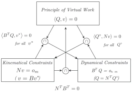
( ) B Q = on -mT Dynamical Constraints Kinematical Constraints

Principle of Virtual Work

for all _{for all}

( )

Figure 1.Duality principle.

where∆◦

Qdenotes the annihilator of∆Q, and Q ◦₌_(Q

1,...,Qm) and Q∗₌_(Q

m₊1,...,Qn) are the generalized force vectors dual to v◦_{and v}∗_{respectively. On the other hand, the input-output} relation between Q◦ and Q∗is reverse to v◦ and v∗; namely,

Q◦is the input and Q∗the output. In the above, the

orthogo-nality condition holds:

BT(q)NT(q)=0.

The matrices N(q) and B(q) are called connection

ma-trices (see Yoshimura, 1995). This orthogonality condition

denotes principle of virtual work, which is given by

hQ,vi=0, for all v∈∆(q) and Q∈∆◦(q), whereh,idenotes a duality pairing.

The dual set of constraints given by Eqs. (4) and (5) in-dicates structural relations, namely, it represents how phys-ical elements are interconnected. Thus, we sometimes call the structural relation an interconnection among the physi-cal elements. In circuit theory, it is known that Eqs. (4) and (5) correspond to KCL and KVL and also that the virtual work principle is known as Tellegen’s theorem. Furthermore, there exists a relation called duality principle as in Fig. 1, which is known as Planck-Okada-Arsove principle in circuit theory (see Yoshimura, 1995).

2.4 Implicit DAEs for Lagrangian systems

Here, we show how the notion of Dirac structures can be fit into the formulation of implicit Lagrangian systems (see Yoshimura and Marsden, 2006a,b, 2008). Let L be a La-grangian on TQ, which is given by

L(q,˙q)=1 2h˙q

◦_,_{M ˙q}◦_{i −}_U(q◦₎_,

(4)

The Lagrange-d’Alembert principle is given by b Z a * d dt ∂L

∂˙q−

∂L

∂q,δq

+

dt+ b

Z

a

hF,δqidt=0,

whereδq satisfies the constraint N(q)δq=om.

So, one can obtain the dual dynamical relation

BT(q)Q=on−m, where

Q= d

dt

∂L

∂˙q−

∂L

∂q+F

and it directly induces

Q= " Q◦ Q∗ # =         

M ˙v◦+f (q◦,v◦)−∂U

∂q◦

τ          , (6) where d dt ∂L

∂˙q−

∂L

∂q =

        

M ˙v◦+f (q◦,v◦)−∂U

∂q◦ 0          and F= " 0 τ # .

Notice thatτindicates the external forces. Of course, equa-tions of motion can be written as

BT(q) d dt

∂L

∂˙q−

∂L

∂q+F

!

=on−m.

Furthermore, one has the second-order condition (see Mars-den and Ratiu, 1999):

˙q◦−v◦=om, (7)

˙q∗−v∗=on−m. (8)

From Eqs. (4), (5), (6), (7) and (8), we can obtain the follow-ing local differential-algebraic equations

G(x(t),˙x(t); u(t))=0, (9)

where x=(q,v,Q)=(q◦_,_q∗_,_v◦_,_v∗_,_Q◦_,_Q∗₎_∈_W_×_W_×_W∗ de-notes the state variables and u=τ∈(Wn−m₎∗₌₍

Rn−m)∗ the input variables. In the above, we locally set TQW×W and T∗_Q

W×W∗, and hence TQ ⊕T∗QW×W×W∗, where

QW=Wm_×Wn−m₌

Rm×Rn−mis an n-dimensional vector space which is a model space forQ. Thus, the mathemati-cal model of the Lagrangian system is given by the implicit DAEs: G=                          G1 G2 G3 G4 G5 G6                          =                         

˙q◦−v◦

˙q∗−v∗ v◦−Jv∗ JTQ◦+Q∗

Q◦−M ˙v◦−f (q◦,v◦)−∂U/∂q◦ Q∗₋_τ

                         . (10)

3 Sparse tableau approach

From the viewpoint of numerical analysis for mechani-cal systems, there exist two kinds of dynamimechani-cal problems; namely, the forward dynamics and inverse dynamics.

Recall that W=Wm×Wn−m=Rm×Rn−mis the model space for Q. The forward dynamics analysis is the case in which given a smooth input vector

u(t) :=τ(t)∈(Wn−m)∗=(_Rn−m)∗

as a vector function of time t, numerically integrate Eq. (9) in terms of t to obtain

x(t)=(q◦(t),q∗(t),v◦(t),v∗(t),Q◦(t),Q∗(t))

as the output, where x∈W×W×W∗. On the other hand, the inverse dynamics analysis is the case in which given a smooth input vector

u(t) :=q∗(t)∈Wn−m=_Rn−m

as a vector function of time t, then compute

x(t)=(q◦(t),v◦(t),v∗(t),Q◦(t),Q∗(t),τ(t))

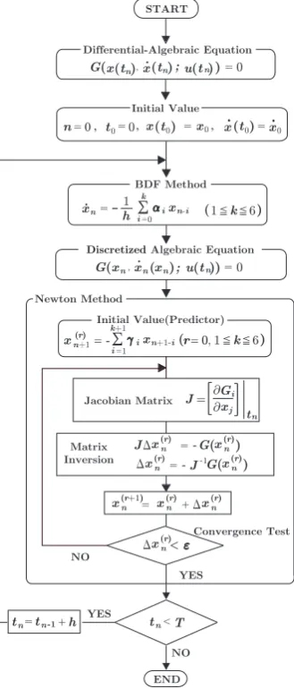
as the output, in which case x∈Wm×W×W∗×(Wn−m)∗. In this paper, we explore the case of the inverse dynam-ics analysis by the sparse tableau approach, where the state vector is given by x=(q◦,v◦,v∗,Q◦,Q∗,τ). To do this, let us first discretize Eq. (9) at time t=tn. By using the

Back-ward Differentiation Formula (BDF) developed by Gear (see,

for instance, Brennen et al., 1995), the time-derivative term ˙xn=˙x(tn) associated to the state vector xn=x(tn) may be ap-proximately discretized by the backwards xn−i=x(tn−i) as

˙xn=− k

X

i=0

1

hαixn−i (1≤k≤6), (11)

where h=tn−tn−1denotes a time step, k is a backward order

andαi indicates the coefficient associated to the i-th back-ward order. Substituting Eq. (11) into Eq. (9), we obtain the discretized nonlinear algebraic equations as follows:

G(xn,˙x(xn); u(tn))=0. (12)

Recall the algorithm of the Sparse Tableau Approach is given in Fig. 2 (see Hachtel et al., 1971; Brayton et al., 1972), where we linearize Eq. (12) at each time step t=tnas

J(x(r)_n )4x(r)_n =−G(x(r)_n ), (13)

and where J=[∂Gi/∂xj]

_t₌_t

nis the Jacobian matrix and

4x(r)n denotes the r-th iterated corrector vector at tn. Then, it fol-lows

x(r_n+1)=x(r)_n +4x(r)_n

(5)

1 0

Differential-Algebraic Equation

Newton Method

Initial Value

BDF Method

Discretized Algebraic Equation

(r)

= r=0;

Initial Value(Predictor)

Jacobian Matrix

Matrix Inversion

NO

YES

NO START

Convergence Test

END

; n

; u(t n)

u(t )

n

(t )

n

(t )

(t 0) (t 0)

x x

G( ) 0

x x0

t 0 0 x x0

i k

h

xn ixn-i (1 k 6)

G(xn xnxn ) 0 ®

xn+1 1

i k+1

ixn+1-i

° ( 1 k 6)

J G_xi

j _t

n

J x(rn) G( (r)

xn) (r)

xn J1G( (r)

xn)

(r+1)

xn (r)

xn

(r)

xn "

tn tn h tn T

( )

@ @

-1

Figure 2.Sparse tableau method.

In the Newton method, it is necessary to take initial values near from the solution xnand the k-th prediction formula xnPr is given by

xPr_n =x(0)_n =−

k

X

i₌1

γixn−i,

whereγiis the i-th coefficient.

In the inverse dynamics analysis, the state vector is given by x=(q◦_,_v◦_,_v∗_,_Q◦_,_Q∗_,τ_{) and it follows from Eq. (10) that} the Jacobian matrix is given as in Fig. 3, where Instands for the n-th degree unit matrix.

4 Bipartite graphs

4.1 Input-output relations

The Jacobian matrix J(x(r)n ) obtained in Eq. (13) apparently has the characteristic of random sparseness. So, we develop

J

Figure 3.Jacobian matrix.

an efficient symbolic generation for computations of the sparse Jacobian matrix inversion for Newton’s iterations. To do this, let us consider an input-output relation among state variables for every relation in (10). Now, we can uniquely allocate the input-output relation to the kinematical and dy-namical relations in Eqs. (4) and (5) as follows:

v◦− Jv∗=om (output : v◦,input : v∗),

JTQ◦+Q∗=on−m(input : Q◦,output : Q∗).

Similarly, for the second-order conditions between v= (v◦_,_v∗_{) and ˙q}₌_{( ˙q}◦_,_˙q∗_{), one has}

˙q◦−v◦=om (output : ˙q◦,input : v◦), ˙q∗−v∗=on−m (input : ˙q∗,output : v∗).

Furthermore, as to the equations of motion, it follows

Q◦−M ˙v◦−f (q◦,v◦)

−∂q◦U=o_m (output : Q◦,input : q◦,v◦),

Q∗−τ=on−m (input : Q∗,output :τ).

The input-output relations in the mentioned above can be de-termined by physical causality. Needless to say that the time derivative terms ˙x(tn) are expressed in terms of the backwards

xn−i(tn),i=0,...,6 by using the BDF as in equation (11). Cor-responding to the Jacobian matrix J in (13), define the causal

Jacobian matrix ˆJ by assigning−1 to the input and+1 to the output as to the j-th variable in the i-th relation associated to

Ji jas

ˆ

Ji j=

        

−1 : the j-th variable is input, +1 : the j-th variable is output,

0 : otherwise.

Thus, the causal Jacobian matrix ˆJ is given in Fig. 4.

In the above,bImindicates the m-th unit matrix. Note that there exists an element with +1 in each row, which plays a role of the pivot in the Gaussian elimination. Further,bIm,n−m is the m×(n−m) matrix, in which+1 are allocated to non-zero components of the m×(n−m) matrixJ.

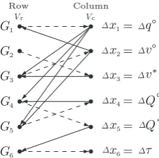
4.2 Oriented bipartite graphs

Let us illustrate the input-output relations as to the Ja-cobian matrix J=[Ji j(x)]=[∂Gi/∂xj]

(6)

J

Figure 4.Causal Jacobian matrix.

bipartite graphs. Recall that the i-th row of the Jacobian

ma-trix J=[Ji j(x)]=[∂Gi/∂xj]

_t₌_t

n corresponds to the i-th vec-tor function Gi(x,˙x; u) and the j-th column corresponds to

j-th vector xj respectively, where i,j=1,...,N(=3n). Here,

Gi(x,˙x; u)=0 are theN-th order DAEs and x=(x1,...,x6)=

(q◦,v◦,v∗,Q◦,Q∗,τ) is theN-vector.

Given the causal Jacobian matrix ˆJ associated to J, let Vr={G1,G2,...,GN} be the row-set of ˆJ and let Vc=

{∆x1,...,∆x6}be the column-set of ˆJ . Here, we assign Vr and Vcto vertex set V :=Vr×Vc.

Now, there are nonzero elements (±1) in the i-th row of the causal Jacobian matrix and suppose that they are in the k-th and l-th columns. For instance, as to the first equation G1=0,

one has the kinematical relation between x1=q◦and x2=v◦

as ˙x1−x2=0. By the BDF discretization, the corresponding

linearized equation is given as

−1

h(α0∆x1)−∆x2=0.

In order to illustrate input-output relations among the state variables by graphs, let us define arc-set by

A={( j,i)|Jˆi j,0,i∈Vc, j∈Vr},

where the arcs represent some relations between vertices in Vc (state variables) as to every vertex (equation) in Vr. Furthermore, the direction of an arc indicates causality or an input-output relation among state variables associated to the column vertices. Let a∈A be an arc. Let us introduce a

map s : A→V, which is given by, for an arc a∈A, s(a)

de-notes the initial vertex of a. Similarly, define a map t : A→V,

which is given by, for an arc a∈A, t(a) indicates the termi-nal vertex of a. So, we can define the set of vertices incident

to a by{s(a),t(a)}. Sometimes, s(a) is called the source of

a and t(a) the target of a. Hence, we can define a directed bipartite graph by

B=(Vr,Vc,A,s,t),

by which we can illustrate the input-output relations

associ-ated to the Jacobian matrix as shown in Fig. 5.

input output

Row Column

V V

x q

v

Q v

Q

*

¿ x1

x2

3

x4

x5

x6 =

=

= G1

G2

G3

G4

G5

G6

r c

G1 x1

x2 a

a 1

2

∆ ∆

∆

Figure 5.Directed bipartite graph.

Row Column Vr Vc

q

v

Q v

Q *

*

¿ x1

x2

x3

x4

x5

x6

=

G1

G2

G3

G4

G5

G6

∆ ∆

Figure 6.Perfect matching.

4.3 Perfect matching

A matching M⊂A of a bipartite graph B=(Vr,Vc,A,s,t) is defined by a set of arcs without common vertices. Especially,

M is called a perfect matching if it is a matching which

matches all vertices of the graph, namely, every vertex of the graph is incident to exactly one edge of the matching: s(M)=

Vrand t(M)=Vc.

In Fig. 6, the arcs that are drawn by the broken lines consist of the perfect matching. If a perfect matching exists in B, the corresponding Jacobian matrix J is a square and nonsingular matrix since|Vr|=|Vc|. Here,|V|means the size of V, namely, the number of elements in the set of vertices V.

Let us see that|V+|=|V−|is equivalent with the fact that the Jacobian matrix is diagonalizable. First, let us show the following relation:

Perfect matchings exist in B⇒J is diagonalizable.

This is clear because a perfect matching can be detected by the elementary row and column operations in matrix; namely, (1) interchanging two rows or columns; (2) adding a multiple of one row or column to another; (3) multiply-ing any row or column by a nonzero element, although there might be several perfect matchings for a given bipar-tite graph. Next, let us show the following relation:

J is diagonalizable⇒Perfect matchings exist in B.

(7)

nonzero elements of the matrix. In other words, the rank of J is equal toN. Recall that a cover is defined as a pair ( ¯Vr,V¯c) of ¯Vr⊂Vr and ¯Vc⊂Vcsuch that there exist no arcs between Vr\V¯r and Vc\V¯c. For the case in which Rank J=

N=|V|/2, the number of the minimum cover for the vertex set V=(Vr,Vc) of the bipartite graph B is to beN. It follows from the K¨onig-Egerv´ary theorem that the number of arcs in a maximum matching is equal to the number of vertices in a minimum vertex cover; namely,

max{|M| |M : matching}

=min{|V¯r|+|V¯c| |( ¯Vr,V¯c) : cover}.

So, the size of the maximum matching is to beN=|V|/2 and therefore we have shown that the matching is a perfect matching. As shown in Fig. 6, there exists a perfect matching

M={a1=(x1,G1),a2=(x2,G3),a3=(x3,G2),

a4=(x4,G5),a5=(x5,G4),a6=(x6,G5)} ⊂A.

For each arc a∈M, one can choose the target x=t(a) as the

pivot associated to the k-th equation, where k=s(a) is the

source of a. Thus, the proof has been done.

Therefore, we can conclude the following relation:

Perfect matchings exist in B⇔J is diagonalizable.

In this way, the solvability of the linearized Eq. (13) is clar-ified in the context of the perfect matching by using the bi-partite graph associated to the causal Jacobian matrix. Recall that nonzero elements of ˆJ correspond to arcs of the

bipar-tite graph and hence the number of nonzero elements and the number of the arcs are the same. In our study, in each row, there is only one output variable, which implies that the arcs

associated with the output variables never share the vertices of other output arcs in the bipartite graph. Therefore, the set

of edges of output variables has perfect matching.

5 Sparse matrix inversion

5.1 Symbolic generation

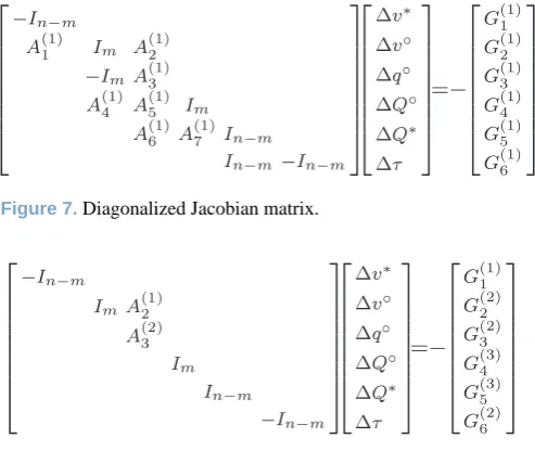
Next, we show how the sparse matrix inversion of the Jaco-bian matrix can be done by symbolic manipulation. By the information from the causal Jacobian matrix, selecting the pivot, the Jacobian matrix can be diagonalized as shown in Fig. 7, where G(k)_{is the k-th tableau error vector, A}(k)

rep-resents a matrix in the Jacobian matrix for the k-th step of elementary operations. Next, after forward Gaussian elimina-tion for the Jacobian matrix, we can easily obtain the reduced Jacobian matrix as in Fig. 8. Note that we can do this by sym-bolic manipulation. Furthermore, after backward elimination as to the reduced Jacobian matrix by symbolic manipulation,

Figure 7.Diagonalized Jacobian matrix.

Figure 8.Reduced Jacobian matrix.

we can obtain the following corrector vector consequently:

∆τ=G(2)₆ ,

∆Q∗=−G(3)₅ ,

∆Q◦=−G(3)₄ ,

∆q◦=−A

(2) 2

G(2)₃ ,

∆v◦=−(G(2)₂ −A(1)₂ ·G(2)₃ ), ∆v∗=G(1)₁ .

Thus, we can develop the inversion of the Jacobian matrix, i.e.,∆x(r)n =−J−1(x

(r)

n )G(x

(r)

n ) can be explicitly done by sym-bolic manipulation with the causal information of ˆJ. As a

result, we can make symbolic generation of Eq. (14).

5.2 Numerical analysis

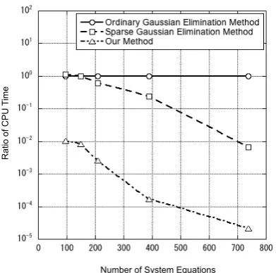
Let us demonstrate the validly of our symbolic generation scheme by an example of the Stanford manipulator with 6 degrees of freedom as shown in Fig. 9. One can set up 96, 150, 210, 390, 738 system equations of DAE models for the stanford manipulator, where the numbers of systems equa-tions correspond to those of the unknown variables according to the elimination of redundant variables.

(8)

Figure 9.Stanford manipulator.

Ratio of CPU

Time

Number of System Equations

Figure 10.Comparison of CPU time.

has a great advantage in the CPU time efficiency in compari-son with other approaches.

6 Conclusions

We have shown symbolic generation of sparse matrix inver-sion for large-scale mechanical systems. We have set up Im-plicit DAE models in the context of Lagrangian systems and we have shown the input-output relations as to the Jacobian matrix associated with linearized equations. Then, we have shown the solvability of the linearized equations by using the bipartite graph. Furthermore, we have proposed symbolic generation of the random sparse matrix inversion for the Ja-cobian matrix. Finally, we have demonstrated the validity of our approach by numerical analysis with an example of the Stanford manipulator comparing with the inner-product sparse matrix Gaussian elimination algorithm as well as the standard Gaussian elimination algorithm.

Acknowledgements. This research is partially supported by JSPS Grant-in-Aid 23560269, JST-CREST, Waseda University Grant for SR 2012A-602 and IRSES project Geomech-246981.

Edited by: A. M¨uller

Reviewed by: two anonymous referees

References

Brayton, R. K., Gustavson, F. G., and Hachtel, G. D.: A new effi -cient algorithm for solving differential-algebraic systems using implicit backward differentiation formulas, Proc. IEEE, 60, 98– 108, 1972.

Brennen, K. E., Campbell, S. L., and Petzold, L. R.: Numerical So-lution of Initial-Value Problems in Differential-Algebraic Equa-tions, Philadelphia, SIAM, 1995.

Hachtel, G. D., Brayton, R. K., and Gustavson, F. G.: The sparse tableau approach to network analysis and design, IEEE Trans. Circuit Theory, CT-18, 101–113, 1971.

Marsden, J. E. and Ratiu, T. S.: Introduction to Mechanics and Sym-metry, volume 17 of Texts in Applied Mathematics, Springer-Verlag, 2nd Edn., 1999.

Murata, T., Oguni, T., and Karaki, Y.: Supercomputer-Application to Scientific Computing, Maruzen, 1985 (in Japanese).

Murota, K.: Matrices and Matroids for Systems Analysis, Springer-Verlag, Berlin, 2000.

Orlandea, N., Chace, M. A., and Calahan, D. A.: A sparsity-oriented approach to the dynamic analysis and design of mechanical sys-tems – Part 1, Part 2, Trans. ASME, J. Eng. Ind., 99, 773–779, 780–784, 1977.

Yoshimura, H.: Dynamics of Flexible Multibody Systems, Ph.D. thesis, Waseda University, Tokyo, Japan, 1995.

Yoshimura, H. and Imai, N.: A sparse tableau approach to dynamics of large-scale nonlinear mechanical systems, IEICE Nonlinear Problems, 103, 39–43, 2004.

Yoshimura, H. and Marsden, J. E.: Dirac structures in Lagrangian mechanics Part I: Implicit Lagrangian systems, J. Geom. Phys., 57, 133–156, 2006a.

Yoshimura, H. and Marsden, J. E.: Dirac structures in Lagrangian mechanics Part II: Variational structures, J. Geom. Phys., 57, 209–250, 2006b.