Replication-based inference algorithms for hard computational problems
Roberto C. Alamino, Juan P. Neirotti, and David Saad
Non-linearity and Complexity Research Group, Aston University, Birmingham B4 7ET, United Kingdom
(Received 13 May 2013; published 31 July 2013)
Inference algorithms based on evolving interactions between replicated solutions are introduced and analyzed on a prototypical NP-hard problem: the capacity of the binary Ising perceptron. The efficiency of the algorithm is examined numerically against that of the parallel tempering algorithm, showing improved performance in terms of the results obtained, computing requirements and simplicity of implementation.
DOI:10.1103/PhysRevE.88.013313 PACS number(s): 05.10.−a, 84.35.+i
I. INTRODUCTION
One of the main contributions of statistical physics to application domains such as information theory and theoretical computer science has been the introduction of established methods that facilitate the analysis of typical properties of very large systems in the presence of disorder. For instance, in information theory applications, these large systems corre-spond to (mostly binary) transmissions where the disorder is manifested through transmission noise or the manner by which the message is generated or encoded. Established approaches in the statistical physics community such as the replica and cavity methods [1] have proved to be useful tools in describing typical properties of error-correcting codes [2–4], the analysis of optimization problems such as the traveling salesman [5], K satisfiability [6], and graph coloring [7,8], to name but a few.
Another important contribution, which complements the ones mentioned above, was in the development of algorith-mic tools to find algorith-microscopic solutions in specific problem instances. One of the most celebrated inference methods, the message-passing (MP) or belief propagation algorithm, had been developed independently in the information theory [9], machine learning [10], and statistical physics [5] communities until the links between them have been identified [11,12] and established [13]. Subsequently, a number of successful inference methods have been devised using insights gained from statistical physics [1,14].
In MP algorithms, the system to be solved is mapped onto a bipartite factor graph, where on the one hand factor nodes correspond to observed (given) information or interaction between variables; while on the other hand are variable nodes, to be estimated on the basis of approximate marginal pseudoposteriors. The latter are obtained by a set of consistent marginal conditional probabilities (messages) passed between variable and factor nodes [1]. Unfortunately, there are many caveats to the MP procedure, especially in the presence of closed loops in the factor graph, which may give rise to inconsistent messages and nonconvergence. It can be shown that MP converges to the correct solution when the factor graph is a tree, but there is no such guarantee for more general graphs, although MP does result in a good solution in many other cases too.
There are two main general difficulties in using MP algo-rithms to problems represented by densely connected graphs. The first is that the computational cost grows exponentially with the degree, making the computation impractical, while
the second arises from the existence of many short loops that result in recurrent messages and lack of convergence. These problems have been solved in specific cases, especially in the case of real observations and continuous noise models by aggregating messages [15]. One of the shortcomings identified in Ref. [15] was nonconvergence when prior knowledge on the noise process is inaccurate or unknown, which typically results in multiple solutions and conflicting messages.
While MP would be successfully applied if a weighted average over all possible states could be carried out, it is clear that such an average is infeasible. Inspired by the state-space representation obtained using the replica method [1,5,16] whereby state vectors are organized in an ultrametric structure, two of us suggested an MP algorithm based on averaging messages over a structured solutions space [17]. The approach is based on using an infinite number of copies (or real replica, not to be confused with those employed in the replica method) of the variables exposed to the same observations (factor nodes). The replicated variable systems facilitate a broader exploration of solution space as long as these replica are judiciously distributed according to the solution-space structure implied by the statistical mechanics analysis. The variable vectors inferred by these algorithms are then combined by taking either weighted or white av-erage to obtain the marginal pseudoposterior of the various variables.
The approach has been successful in addressing the code division multiple access (CDMA) problem as well as the linear Ising perceptron capacity problem [18], even in cases where prior information is absent. It is worthwhile noting that a seed of this replication philosophy can be found in several previous algorithms such as (a) query by committee
It is interesting to note that approaches based on averaging multiple interacting solutions have also been successfully tried in neighboring disciplines, for example, for decoding in the context of error-correcting codes [24].
While this approach has been successful in addressing inference problems in the case of real observations and continuous noise models, it is less clear as to how it could be extended to accommodate more general cases. In this work, we will present an alternative method for carrying out averages over the replicated solutions, which can be applied to more general cases. Generally, like most MP-based algorithms, the approach is based on solutions being calculated iteratively using a pair of coupled self-consistent equations. We will study the properties of this alternative algorithm, its advantages and limitations, on an exemplar problem of the binary Ising perceptron (BIP) [25,26] that has been used as a benchmark also in other works on advanced inference methods [27].
One obvious obstacle in most MP algorithms is that the iterative dynamics can be trapped in suboptimal minima; in addition, the algorithm itself can either create spurious suboptimal minima in the already complex solution space or change the height of the energy barriers between the existing ones. We will show that our replica-based MP algorithm fails under naive averaging of the replica for the BIP capacity problem, explain analytically why it happens, and show that in the limit of a large number of replica, averages flow to the clipped Hebb algorithm [26]. We will then propose an alternative approach and show how replication can indeed improve performance if carried out appropriately.
In Sec. II, we will explain the exemplar problem to be used in this study; we will then review the nonreplicated MP solution to the BIP capacity problem under the approximation for densely connected systems in Sec. III and provide an analytical solution to the naively replicated MP algorithm, showing here its equivalence with the clipped Hebb rule. Sec-tionIVwill point to the main reason for the failure of the naive replica-averaging approach and argue that an online version of the MP algorithm, which is derived and presented, can solve it. By replicating the new online MP (OnMP) algorithm and using the extra degrees of freedom that it provides, we show how it outperforms the nonreplicated MP algorithm, termed offline MP (OffMP) algorithm. Section V compares the replicated OnMP (rOnMP) with a benchmark parallel algorithm, namely, the PT algorithm. Finally, conclusions and future directions are discussed in Sec.VI.
II. EXEMPLAR PROBLEM: THE BINARY ISING PERCEPTRON
To extend the replica-based inference method [18], we would like to use an exemplar problem that is particularly difficult, not only in the worst-case scenario but also typically where both observations and noise model are not real valued. In addition, we would like to examine a case where exact results have been obtained by the replica theory; this provides helpful insight in devising the corresponding algorithm by suggesting a possible structure for the solution space as well as an analytical tool to assess the efficacy of the algorithm.
One prototypical NP-complete problem [28] that was shown to be computationally hard even in the typical case, which was solved exactly using the replica method, is the capacity of the binary Ising perceptron [25]. This is due to the complex structure of its solution space studied in Ref. [29], showing a nontrivial topology even in the replica symmetric (RS) phase.
The BIP [26] represents a process wherebyK-dimensional binary input vectorssμ∈ {±1}Kare received, where the input vector indexμ=1, . . . ,N, represents each of theNexample vectors. The corresponding outputs for each one of them is determined by the binary classification
yμ=sgn
1
√
K
K
k=1 sμkbk
, (1)
whereb=(b1, . . . ,bK)∈ {±1}Kis called the unknown binary
variables (also referred to as the perceptron’s variable vector); the prefactor√Kis for scaling purposes, so that the argument of the sign function remains orderO(1) asK→ ∞.
The capacity problem for a BIP is a storage problem, although it can alternatively be seen as a compression task [30]. In the simplest version of the problem, a data set D= {(sμ,yμ)}Nμ=1consisting ofNpairs of inputs and outputs (also calledexamples) is randomly generated and a perceptron with an appropriate variable vector bshould be found, such that when presented with an input patternsμ, it reproduces the corresponding outputyμ. That is the equivalent of compressing
the information contained in the set of classifications {yμ},
comprising N bits, into a vector bwith onlyK bits. One is usually interested in the typical case, which is calculated by averaging over all possible data setsDdrawn at random from a certain probability distribution.
Typical performance is algorithm dependent and is mea-sured by counting the fraction of correctly stored patterns as a function of the number of examples in the data set. One convenient measure is the average value of the indicator function
χ( ˆb)=1−
N
μ=1
yμ
1
√
K
K
k=1 sμkbˆk
, (2)
with (· · ·) being the Heaviside step function and ˆb the inferred variable vector. This measure gives 0 if all examples are correctly stored and 1 otherwise, i.e., it is indicating that all patterns were perfectly memorized. The maximum value of α=N/K for which this cost function is 0 (averaged over all possible data sets) is the achieved capacity of the algorithm and a measure of its overall performance. This indicator function was chosen because the BIP capacity problem focuses on perfect inference of the perceptron’s variable vector b, without allowing for any distortion, or noise, in the patterns classification. Additionally, it is the most commonly used measure in recent publications in this field (e.g., in Ref. [27]).
by the number of misclassified patterns
E( ˆb)=
N
μ=1
−yμ
1
√
K
K
k=1 sμkbˆk
. (3)
Alternative energy functions were suggested in the liter-ature, for instance [31], and were used in various contexts, especially in the machine learning literature. While the different energy functions tend to share a joint ground state, they may exhibit different behaviors under noisy conditions (imperfect learning, at finite temperatures) as they correspond to different noise models. Although the study of algorithmic performance at higher temperatures is interesting, it is not within the scope of this work, which focuses on examining the performance of the suggested algorithm against results obtained for the benchmark problem of perfect storage at the noiseless, zero temperature limit.
It should be noted that the distribution of patterns to be memorized affects the performance of the algorithm. Within the class of solvable Ising perceptron capacity problems, patterns sampled from an unbiased distribution constitute the most difficult task. Biased patterns are less informative and are therefore easier to store [32]. We will therefore study only patterns generated from unbiased distributions, representing the most difficult problem, but the method could clearly be extended to accommodate biased patterns.
Although the achieved capacity varies between algorithms, there is an absolute upper bound, the critical capacityαc, above
which no algorithm can memorize the whole set of examples in the typical case (although it might be possible for specific instances); this reflects the information content limit of the perceptron itself.
The critical capacity was calculated by Krauth and M´ezard using the one-replica symmetry breaking (1RSB) ansatz [25] with the result ofαc≈0.83. Taking into consideration that the
problem is computationally hard, the challenge then becomes to find an algorithm which infers appropriatebvalues in typical specific instances ofD as close as possible toαc, where the
corresponding computational complexity scales polynomially with the system size.
III. NAIVE MESSAGE PASSING
The inference problem we aim to address is finding the most appropriate value of the variable vector b capable of reproducing the classifications given the examples data setD. First, one needs to determine a quality measure that quantifies the appropriateness of a solution. The most commonly used error measure in similar estimation problems is the expected error per variable, or bit-error-rate in the information theory literature, the minimization of which leads to a solution based on the marginal posterior maximizer (MPM) estimator given by
ˆ
bk=argmaxbk∈{±1}
bl=k
P(b|D)=sgnbk P(b|D), (4)
which means that one estimates b bitwise, such that each component ˆbkcorresponds to the variable value that maximizes
the marginal distribution per variable given the data setD. The
MP equations allow one to carry out an approximate Bayesian inference procedure to find this estimator.
It is important to remember that there might not exist a variable vector capable of reproducing the whole data set. In this case, the data set is unrealizable by the BIP, although one can still identify the most probable candidate. In the BIP capacity problem, unrealizable data sets exist since they are generated randomly, not by a teacher perceptron as is the case in some generalization problems. Each variable in the setDis drawn from an independent distribution and therefore one can write the posterior distribution of the variable vector as
P(b|D)=P(b|{yμ},{sμ})∝P({yμ}|b,{sμ})P(b), (5)
whereP({yμ}|b,{sμ}) factorizes as the examples are sampled
identically and independently
P({yμ}|b,{sμ})= N
μ=1
P(yμ|b,sμ). (6)
From the Bayesian point of view, P(b) is interpreted as the (factorized) prior distribution of possible variable vectors. As there is no noise involved in the capacity problem, the likelihood factor is simply given by
P(yμ|b,sμ)=
1 2+
yμ
2 sgnξμ, (7) defining
ξμ=
1
√
K
K
k=1
sμkbk. (8)
As for each instance the data set is fixed, we will omit in the following expressions the explicit reference to the input vectorssμin the posterior distribution for brevity.
The resulting MP equations are self-consistent coupled equations of marginal conditional probabilities which are iterated until convergence (or up to a cutoff number of iterations). These equations are obtained by applying Bayes theorem to each one of the so-called Q messages and R messages
Qtμk+1(bk)=Pt+1(bk|{yν=μ})
∝P(bk)
ν=μ
Pt+1(y
ν|bk,{yσ=ν}), (9)
Rtμk+1(bk)=Pt+1(yμ|bk,{yν=μ})
=
{bl=k}
P(yμ|b)
l=k
Pt
(bl|{yν=μ}), (10)
whereP(bk) is the prior distribution over thekth entry of the
variable vector andtstands for the current iteration step. Asbk∈ {±1}, one can write
Qt(bk)=
1+mtμkbk
2 and R
t
(bk)∝
1+mˆtμk−1bk
2 . (11) The variablesmμkmay be interpreted as magnetization related
to the cavity field in analogy to spin lattices in magnetic fields. The interpretation of the ˆmμkvariables is less intuitive.
MP equations in their well-known form
ˆ mtμk=
bkbkP
t+1(y
μ|bk,{yν=μ})
bkP
t+1(y
μ|bk,{yν=μ})
, (12)
mtμk =tanh ⎡ ⎣
ν=μ
atanh ˆmtνk ⎤ ⎦≈tanh
⎛ ⎝
ν=μ
ˆ mtνk
⎞ ⎠. (13)
The approximation in the last equation is possible since ˆmμk ∼
O(1/√K) as we will see later.
Once convergence is attained, the value for the variable vector can be estimated by
ˆ
bk=sgnmk, (14)
mk =tanh
ν
ˆ mtνk
, (15)
or
ˆ bk=sgn
ν
ˆ mtνk
. (16)
As mentioned in Sec. II, the factor graph representing the BIP is densely connected, but an expansion for largeK suggested by Kabashima [15] helps to simplify the equations away from criticality. However, for the BIP this expansion requires extra care due to the discontinuity of the sign function. To address this problem, we developed a different approach to carry out this expansion which can be generalized to accommo-date other types of perceptrons with minimal modifications; it can be applied to either continuous or discontinuous activation functions, with or without noise. Equation(13)formμkis not
modified, but ˆmμk is expanded in powers of 1/
√
K, giving rise to a different expression (detailed derivation is provided in AppendixA):
ˆ mμk=
2sμkyμ
√
K
Nμk
1+erfyμuμk/
2σ2
μk
, (17)
where
Nμk=
1
2π σμk2
exp
−u
2
μk
2σ2
μk
, (18)
σμk2 = 1 K
l=k
1−m2μl, (19)
uμk=
1
√
K
l=k
mμlsμl. (20)
However, this version of the algorithm is unable to memorize large numbers of examples. Simulation results show that, even for small system sizes (K∼10), it can not memorize more than a single pattern on average. This is a consequence of the fact that the dynamical map defined by the MP equations becomes trapped in the many suboptimal minima of the energy landscape.
In principle, one should be able to correct this by replicating the system and distributing thenreplica randomly in solution space, let each one carry out the inference task independently, and compare their final fixed points. An idea along these lines, with a small number of real replica searching the space in parallel, was tested with some success in Ref. [21], where the
replica helped change the landscape to facilitate jumps over barriers between metastable states. However, the correspond-ing algorithm was not very efficient computationally. Also, the replicated version of MP we tested failed and the observed performance coincided with that of the nonreplicated version. To understand the reasons for the failure of the naively replicated algorithm, we solved the replicated version of the algorithm analytically. We consider the case where a simple white average of thenreplica is used for inferring the variable vector value
ˆ bk=sgn
1 n
n
a=1 bak
. (21)
We can then evaluate the MP equations using a saddle point method whenn,N,K → ∞. The detailed calculation is given in AppendixB, giving rise to a surprisingly simple final result
ˆ bk=sgn
⎛ ⎝N
μ=1 yμsμk
⎞
⎠. (22)
Simplicity is not the only surprising aspect of this result. Those familiar with past research in machine learning will readily recognize this equation as the clipped version of the Hebb learning rule [33]. Unfortunately, this is not good news as the maximum attainable capacity by this algorithm has been already calculated analytically to be NH
K ≡αH = ≈0.11 [34,
35]. Worse yet, the achieved capacity of the clipped-Hebb rule quickly deteriorates as K increases, converging to zero asymptotically.
The flow of the replicated algorithm towards the clipped Hebb rule points out some other weaknesses of the MP algorithm. It is not difficult to appreciate that MP results in a clipped rule as the final estimate of the variable vector is obtained by clipping the fixed point of the magnetization; this implies that it suffers from all pathologies present in clipped rules such as suboptimal solutions.
Another characteristic that is highlighted by this result is the fact that, like the Hebb rule, the MP approach is an offline (batch) learning algorithm in the sense that it does not depend on the order of presentation of the examples. This is true both for the nonreplicated and replicated algorithms. This suggests that one could introduce an extra source of stochasticity by devising an online version of the MP, which could allow for the algorithm to overcome the energy barriers that trap it in local minima. Different orders of examples correspond to different paths in solution space which, combined, could potentially explore it much more efficiently. The examples order is an extra degree of freedom that can not be exploited in offline algorithms. In the following section, we show that by pursuing this idea, we find a replicated version of MP which does not only perform better than the offline one (OffMP), but also offers many additional advantages.
IV. ONLINE MESSAGE PASSING
exploit the order of presentation of examples as a mechanism to avoid algorithmic trapping in local minima. This algorithm will then be used in its replicated version with a polynomial number of replicanwith respect to the number of examples N.
In order to develop an online version of the MP algorithm, we rely on a large K expansion. When K→ ∞, one can derive the equations for the magnetization (mean values) of the inferred variable vector [Eq.(15)] as
mk=tanh
ν
ˆ mνk
=tanh ⎛ ⎝
ν=μ
ˆ
mνk+mˆμk
⎞ ⎠
≈tanh ⎛ ⎝
ν=μ
ˆ mνk
⎞ ⎠+mˆμk
⎡
⎣1−tanh2 ⎛ ⎝
ν=μ
ˆ mνk
⎞ ⎠ ⎤ ⎦
=mμk+[1−(mμk)2] ˆmμk. (23)
Equation (23) singles out the μth example similarly to the OffMP derivation. However, in the online interpretation it is considered anew example, being presented sequentially after all previous μ−1 examples have been learned. Then, mk can be interpreted as the updated magnetization, while
mμk is the magnetization linked to the cavity field induced
by the previous examples, before example μ is included. In the bipartite interpretation of the model, this is akin to the introduction of new a factor node, exploiting conditional probabilities calculated with respect to the previous μ−1 examples. To make this interpretation more explicit, we add a time label to the obtained equation by changingmktomk(t),
mμk to mk(t−1), and considering the μth example as the
example being presented at timet. The online MP algorithm can finally be written as
mk(t)=mk(t−1)+
stkyt
√
KFk(t), (24) with the so-calledmodulation functiongiven by
Fk(t)=2
1−m2k(t−1) Ntk 1+erfytutk/
2σ2
tk
, (25)
where
σtk2 = 1 K
l=k
1−m2l(t−1), (26)
utk=
1
√
K
l=k
stlml(t−1). (27)
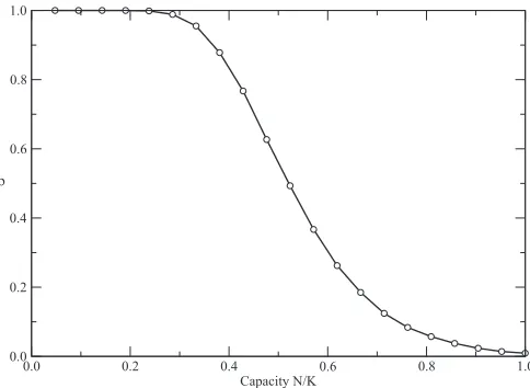
The performance of the OnMP algorithm without replica-tion is shown in Fig.1forK=21 averaged over 200 different sets of examples. The vertical axis showsρ=1− χ , the average value of the function that indicates perfect learning. However, becauseχ ∈ {0,1}we have to estimate the variance by repeating the average several times and calculating an average over averages. For the graph of Fig.1, this was done 200 times for each particular data set and the corresponding
0.0 0.2 0.4 0.6 0.8 1.0
Capacity N/K 0.0
0.2 0.4 0.6 0.8 1.0
ρ
FIG. 1. Nonreplicated online version of the MP algorithm. While the offline MP can not learn perfectly more than one single example, we see that the OnMP can, already without replication, memorize perfectly a larger number of examples. The vertical axisρ is the average value of the indicator function that gives 1 if all patterns are memorized and 0 otherwise. The horizontal axis is the capacity α=N/K.
error bars are smaller than the size of the symbols. We see that, contrary to the OffMP, the online version is now able to memorize perfectly a larger number of examples on average, with a larger achieved capacity. The slow decay to zero is to be interpreted as a finite size effect, which is however difficult to since increasing the system sizeKleads to a deterioration of performance instead of a sharper transition.
Let us now replicate this algorithm. For N examples, there are N! possible orders of presentation, but we will choose only a number n of these sequences, with n being of polynomial order inN. We will see that this is enough to improve considerably the performance of the algorithm. We compare two versions of the replicated algorithm with white and weighted average over replica. Both versions work by exposing the n replica independently to different orders of examples. To minimize residual effects, we allow a relearning procedure with L∼10 relearning cycles while keeping the same order of presentation. As the MP algorithm relies on clipping, it shows a poorer performance when the number of examples is small, especially for the even cases where parity effects are amplified. This effect, however, disappears as N grows larger.
The difference between the white and weighted algorithms lies in how the final estimate for the variable vector is calculated. Respectively, we have
ˆ
bwhitek =sgn
1 n
n
a=1 bka
, (28)
ˆ
bweightedk =sgn n
a=1 wabak
, (29)
where
wa∝e−βE(ba), (30)
high value in order to select lower energy states. Clearly, when β=0, the white and weighted averages are the same.
We compared the performance of the two versions of the rOnMP against the nonreplicated one. Both perform much better than the nonreplicated algorithm. The difference between weighted and white averages in related problems had already been studied in relation to the TAP equations via the replica approach yielding similar results [20]; this indicates that similar problems appear in the corresponding dynamical maps. Contrary to our expectations, though, we have not found any difference in performance between the weighted and white averaged algorithms. This seems to indicate that even selection of the best performers as done by the weighted average is not enough to prevent the algorithm of being trapped in suboptimal solutions, which can only be avoided by increasing the number of replica.
It is interesting to note that a variational approach carried out by Kinouchi and Caticha [36] was successful in finding the optimal online learning rule for a perceptron, in the sense that it will saturate the Bayes’ generalization bound calculated by Opper and Haussler [37]. Although the perceptron generaliza-tion problem is different from the capacity problem, as in the former, the data set is clearly realizable having been generated by a corresponding perceptron, which might not be the case for the latter; up to the critical capacity one can assume that the set of random examples, in the typical case, is indeed realizable. In fact, this is usually one of the underlying assumptions when attempting to solve the capacity problem. This means that we can use the same algorithms to carry out both tasks.
The precise form for the parallel variational optimal (VO) algorithm for the BIP was derived in Ref. [38] and is given by
b(t+1)=b(t)+√styt
NF(t), (31)
where the modulation function is
F(t)=2
Q(t)
R(t)2[1−R(t) 2]
× Nt
1+erf(R(t)φ(t)/2(1−R(t)2)), (32) with
R(t)= b0·b(t)
|b0||b(t)|
, Q(t)= b(t) 2
N ,
(33) φ(t)=h(t)yt, h(t)=
b·st
|b| ;
where b0 is a teacher perceptron, which in the capacity case would correspond to the correct inferred variable vector, the true value of which we do not know. In employing the VO algorithm, an assumption that the overlaps are self-averaging has been used. Therefore, a sensible way to obtain a value that could be used as a good estimate ofb0is to run the algorithm many times in parallel and average all values ofb(t) at each iteration. Like in our algorithm, this average can be either white or weighted.
A notable characteristic of the above set of equations is their similarity with our equations for the OnMP if one substitutes
mk→bk, m2k→R2, Rφ→yu, 1−R2→σ2, (34)
respectively. In fact, the asymptotic behavior of the VO guarantees that even the square-root amplitude appearing in front of the modulation function tends to the same value as in the OnMP, making the two sets isomorphic under this substitution. This striking relation between both algorithms is a strong indication that our algorithm must also be capable of achieving the optimal capacity and saturates Bayes’ generalization bound [37].
V. PERFORMANCE
In this section, we compare the performance of the rOnMP with that of the PT algorithm. The reason for choosing PT is that it is a well established parallel algorithm with good performance in searching for solutions in the BIP capacity problem. Other derivatives of BP-based algorithms have been used to solve the BIP capacity problem, for instance, survey propagation [6,27]; the latter also aims to address the fragmentation of solution space but employs a different approach. The results reported [6,27] show that solutions can be found very close to the theoretical limits even for large systems, but additional practical techniques and considerations should be used to successfully obtain solutions. As our aim in this work is to show how replication can improve significantly the performance of MP algorithms, we use the PT algorithm as the preferred benchmark method due to its simpler implementation.
Parallel tempering (PT) or replica exchange Monte Carlo algorithm [22,23] was introduced as a tool for carrying out simulations of spin glasses. Like the BIP capacity problem, spin glasses have a complicated energy landscape with many peaks and valleys of varying heights and PT has been successfully applied to that and many other similar problems where the extremely rugged energy landscape causes other methods to underperform [39,40].
In many cases, searching for the low energy states is done by gradient descent methods. In statistical physics, simulated annealing is a principled and useful alternative to gradient descent by allowing for a stochastic search while slowly decreasing the temperature; it is particularly effective in the cases where the landscape has one or very few valleys. However, to guarantee convergence to an optimal state, the temperature should be lowered very slowly and most applications use a much faster cooling rate. In the case of spin glasses, this causes the algorithm to be easily trapped in local minima.
0.5 1.0 1.5
α
0.0 0.2 0.4 0.6 0.8 1.0
ρ
Parallel Tempering Online MP / n=10000
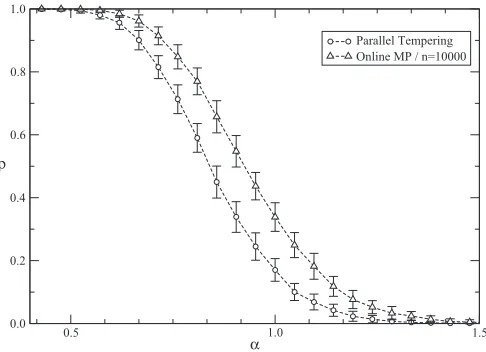
FIG. 2. Results from the parallel tempering algorithm (circles) versus the replicated online MP (triangles) with 10 000 replica. The system size isK=21. The graph, presented with error bars over 10 000 trials, shows the superiority of the MP already for this number of replica.
this probability is given by the ratio of the Boltzmann weights as in the usual Metropolis-Hastings algorithm.
As time proceeds, the lowest energy walker corresponds to the lowest-temperature replica. After convergence or when a certain number of iterations have been done, results for all temperatures can be obtained. PT has a very high performance for the BIP capacity problem and can achieve very high storage capacities. The disadvantage comes from the fact that PT uses much more information than is needed to solve the BIP capacity problem and is therefore computationally expensive. Figure2 shows the performance of the rOnMP compared to PT for a system sizeK=21. The graph shows, once again, the same indicator function used for rOnMP ρ=1− χ , whereχ is given by Eq.(2). The energy function used in the actual PT simulation was the energy given by Eq.(3). We see that already withn=10 000 replica rOnMP has a better performance than PT, which was run up to the point when there was no extra improvement. We observed that by increasing the number of replica, we can reach better performances although the improvement in the performance becomes more modest for higher values; studies with a large number of replican∼ 105 seem to indicate that the critical capacity can indeed be achieved fornsufficiently large. However, the computing time increases as well and more lengthy and detailed analysis is necessary to get precise results.
It is also important to know how increasingK affects the performance of the algorithm. Due to the complex energy landscape of the BIP problem, the larger the system size, the larger the probability of being trapped in the increasing number of local minima. This has been observed in various studies concerning learning via random walks as explained in Ref. [41]. Further experiments with our method on the BIP problem seem to indicate that in the many-replica case, the algorithm’s performance does not deteriorate with increasing K, the achieved performance showing little sensitivity to the value ofK. The main effect noticed was that finite size effects decrease with increasingK, making the transition from perfect
to partial learning sharper. The corresponding computing time increases quadratically withK.
In addition to the better performance, rOnMP has several other advantages over PT. First, the running time for achieving a similar performance is lower. Second, and more importantly, PT depends on a complicated fine tuning of the number of replica at different temperatures and how these are spaced. Different ranges of temperatures and spacings between them give different results and these require optimization trials. On the other hand, the application of rOnMP is much more straightforward and depends only on the number of replica.
VI. CONCLUSIONS
The main objective for this work was to show that parallelizing message passing algorithms, via replicationof the variable system, can lead to a dramatic improvement of their performance. Replication is based on insights and concepts from statistical physics, especially in the subfield of disordered systems. The binary Ising perceptron (BIP) capacity problem was chosen as a difficult benchmark problem due to its complex solution space and its discrete output and noise model; both make the inference problem particularly difficult.
First, we showed analytically that the offline version of the MP algorithm for the BIP capacity problem results in the clipped Hebb rule estimator in the thermodynamic limit and when the number of replica is large. This shows a fundamental limitation of the MP procedure and motivated us to search for an online version of it; after establishing the single system version, it has been extended to accommodate a replicated version. Both the nonreplicated and the replicated versions were shown to have superior performance to that of the OffMP.
There are two important aspects of replicated algorithms we would like to point out, namely, the way the search is carried out in solution space and how to combine the search results to obtain a unified estimate. We devised a method to make replicated variable systems follow different paths in the solution space by using different orders of example presentations, which is only possible in online algorithms. We also tried two different ways to combine the results, white and weighted averaging, the latter using the Boltzmann factors of each replica. We found no difference between both approaches, indicating that weighting the averages is not sufficient to avoid local minima.
to the replica symmetry breaking solution space and demands the introduction of a carefully constructed interaction between the replicated solutions, which we currently investigate.
ACKNOWLEDGMENT
Support by the Leverhulme trust (F/00 250/M) is acknowl-edged.
APPENDIX A: MESSAGE PASSING EXPANSION FOR THE BINARY ISING PERCEPTRON
Consider the first MP equation(12), repeated as follows for convenience:
ˆ mtμk =
bkbkP
t+1(y
μ|bk,{yν=μ})
bkP
t+1(y
μ|bk,{yν=μ})
. (A1)
We denote the numerator of this expression simply by A, ignoring for brevity the dependence on the indices. By introducing a variableξto represent the fieldξμusing a Dirac
delta, we can write
A= yμ 2K
dξ dξˆ
2π e
iξξˆ (sgnξ)
×
⎡ ⎣
l=k
b
(1+mμlb) exp
−iξˆs√μlb K ⎤ ⎦ × b b exp
−iξˆs√μkb K
. (A2)
Summing overb∈ {±1}, one obtains
b
(1+mμkb) exp
−iξˆs√μkb K =2 cos ˆ ξ √ K
−imμksμksin
ˆ ξ √ K ≈2
1−imμksμk
ˆ ξ √ K − ˆ ξ2 2K , (A3)
where, in the last line, we expand the trigonometric functions to their first nontrivial orders in 1/√K, already taking into
consideration the large K scenario. By doing the same expansion to the second summation, one obtains
b
b exp
−iξˆs√μkbk K
= −2isμksin
ˆ ξ
√
K
≈ −2isμk
ˆ ξ
√
K. (A4)
These approximations allow one to rewrite the expression forAas
A= −iy√μsμk K
dξ dξˆ
2π e
iξξˆ
(sgnξ) ˆξ
×exp l ln
1− ξˆ 2
2K −imμlsμl ˆ ξ
√
K
≈ −iyμsμk
√
K
dξ 2π (sgnξ)
dξˆξˆ
×exp
−ξˆ
2σ2
μk
2 +iξˆ(ξ−uμk)
, (A5)
where
σμk2 = 1 K
l=k
1−m2μl, uμk=
1
√
K
l=k
mμlsμl. (A6)
The resulting integral is trivial and, by following the analogous steps for the denominator, we finally reach the result given by expression(17).
APPENDIX B: ANALYTICAL DERIVATION OF THE REPLICATED NAIVE MP ALGORITHM
Upon replication of the variable system such that the final estimate of the variable vector is inferred by a white average of thenreplica
ˆ bk=sgn
1 n
n
a=1 bka
, (B1)
one can take the limitn→ ∞to calculate a closed expression for it. The MP equations(12)and(13)remain the same, but the likelihood term has to include the contribution of the replica as
P(yμ|b)=
{ba}
P(yμ|b,{ba})P({ba}|b), (B2)
P(yμ|b)=
1 2n+1
1+yμsgn
1 √ K K
k=1 sμkbk
a
1+yμsgn
1 √ K K
k=1 sμkbak
, (B3)
P({ba}|b)∝
k
1 2
1+bksgn
1 n
n
a=1 bka
. (B4)
be written as
A∝ dξ dξˆ 2π e
iξξˆ
a
dξadξˆa
2π e
iξaξˆa
(1+yμsgnξ)
a
(1+yμsgnξa)
b bk
⎡ ⎣
l=k
1
2(1+blmμl) ⎤ ⎦exp
⎡ ⎣−√iξˆ
K
K
j=1 sμjbj
⎤ ⎦
×
{ba}
j
1 2
1+bjsgn
1 n
n
a=1 bja
exp
⎡ ⎣−√i
K a ˆ ξa K
j=1 sμjbja
⎤
⎦. (B5)
To decouple the replicated systems, we introduce theKvariables
λk=
1 n
a
bak, (B6)
via Dirac deltas. By defining the notation
D[ξ,ξˆ]≡
dξ dξˆ 2π e
iξξˆ
a
dξadξˆa
2π e
iξaξˆa
, D[λ,λ]ˆ ≡
k
dλkdλˆk
2π/n e
inλkλˆk
, (B7)
and summing overb’s, we obtain
A∝
D[λ,λ]D[ξ,ˆ ξˆ](1+yμsgnξ)
a
(1+yμsgnξa)
⎡ ⎣ a,j cos ˆ λj+
ˆ ξas
μj
√
K ⎤
⎦−isin ˆ
ξ sμk
√
K
+sgnλkcos
ˆ ξ sμk
√
K
×
l=k
(1+mμlsgnλl)
cos
ˆ ξ sμl
√
K
−isgnλlsin
ˆ ξ sμl
√
K
. (B8)
One can now expand the arguments of the cos and sin functions in powers of 1/√Kto obtain
A∝
D[λ,λ]D[ξ,ˆ ξˆ](1+yμsgnξ)
a
(1+yμsgnξa) exp
⎡ ⎣
a,j
ln
cos ˆλj−
ˆ ξasμj
√
K sin ˆλj − ( ˆξa)2
2K cos ˆλj ⎤
⎦
×
−iξ s√ˆ μk
K +sgnλk
exp ⎡ ⎣
l=k
ln(1+mμlsgnλl)+
l=k
ln
1− ξˆ 2
2K − iξˆ
√
Ksgnλl ⎤
⎦. (B9)
The integrals over theξvariables are easy to calculate, leading to the following expression at leading order in 1/√K:
A∝ ⎡
⎣
j
dλjdλˆj
2π/n ⎤
⎦sgnλken, (B10)
where
=i
j
λjλˆj +
1 n
l=k
ln (1+mμlsgnλl)
+
j
ln cos ˆλj +
1 n
n
c=0
lnIc, (B11)
with
Ia=1+yμerf
⎛ ⎝ uμ
2σ2
μ
⎞
⎠, a=1, . . . ,n (B12)
uμ= −
i
√
K
j
sμjtan ˆλj, (B13)
σμ2= 1 K
j
1+tan2λˆj
, (B14)
I0 =1+yμerf
u0 μk √ 2 , (B15)
u0μk= √1 K
l=k
sμlsgnλl. (B16)
Following the same calculations for the denominator, one can see that for largenthe variables ˆmμkare given by sgnλ∗k,
whereλ∗kis defined by the saddle point of the integral(B10), which is a solution of the simultaneous equations
∂ ∂λj
= ∂
∂λˆj
=0. (B17)
Differentiatingwe finally find the result
ˆ
mμk=yμsμk, (B18)
[1] M. M´ezard and A. Montanari, Information, Physics, and Computation(Oxford University Press, Oxford, UK, 2009). [2] D. Saad, Y. Kabashima, T. Murayama, and R. Vicente, in
Cryptography and Coding, Lecture Notes in Computer Science, edited by B. Honary, Vol. 2260 (Springer, Berlin, 2001), pp. 307–316.
[3] R. C. Alamino and D. Saad,Phys. Rev. E76, 061124 (2007). [4] R. C. Alamino and D. Saad,J. Phys. A: Math. Theor.40, 12259
(2007).
[5] M. M´ezard and G. Parisi,J. Phys. (Paris)47, 1285 (1986). [6] A. Braunstein, M. M´ezard, and R. Zecchina,Random Struct.
Alg.27, 201 (2005).
[7] J. van Mourik and D. Saad,Phys. Rev. E66, 056120 (2002). [8] R. Mulet, A. Pagnani, M. Weigt, and R. Zecchina,Phys. Rev.
Lett.89, 268701 (2002).
[9] R. G. Gallager, Research Monograph Series, 21(MIT Press, Cambridge, MA 1963).
[10] J. Pearl,Probabilistic Reasoning in Intelligent Systems: Net-works of Plausible Inference(Morgan Kaufmann, San Francisco, 1988).
[11] Y. Kabashima and D. Saad,Europhys. Lett.44, 668 (1998). [12] M. Opper and D. Saad,Advanced Mean Field Methods-Theory
and Practice(MIT Press, Cambridge, MA, 2001).
[13] J. S. Yedidia, W. T. Freeman, and Y. Weiss,IEEE Trans. Inf. Theory51, 2282 (2005).
[14] M. M´ezard, G. Parisi, and R. Zecchina,Science297, 812 (2002). [15] Y. Kabashima,J. Phys. A: Math. Gen.36, 11111 (2003). [16] H. Nishimori,Statistical Physics of Spin Glasses and
Informa-tion Processing(Oxford University Press, Oxford, UK, 2001). [17] J. P. Neirotti and D. Saad,Europhys. Lett.71, 866 (2005). [18] J. P. Neirotti and D. Saad,Phys. Rev. E76, 046121 (2007). [19] H. Seung, M. Opper, and H. Sompolinsky, in COLT ’92
Proceedings of the Fifth Annual Workshop on Computational Learning Theory(ACM, New York, 1992), pp. 287–294.
[20] C. De Dominicis, M. Gabay, T. Garel, and H. Orland,J. Phys. (Paris)41, 923 (1980).
[21] J. Kurchan, G. Parisi, and M. A. Virasoro,J. Phys. I (France)3, 1819 (1993).
[22] R. H. Swendsen and J.-S. Wang, Phys. Rev. Lett. 57, 2607 (1986).
[23] E. Marinari and G. Parisi,Europhys. Lett.19, 451 (1992). [24] S. Kudekar, T. J. Richardson, and R. L. Urbanke,IEEE Trans.
Inf. Theory57, 803 (2011).
[25] W. Krauth and M. M´ezard,J. Phys. (Paris)50, 3057 (1989). [26] A. Engel and C. van den Broeck, Statistical Mechanics of
Learning(Cambridge University Press, Cambridge, UK, 2001). [27] A. Braunstein and R. Zecchina,Phys. Rev. Lett. 96, 030201
(2006).
[28] L. Pitt and L. G. Valiant, J. Assoc. Comput. Mach.35, 965 (1988).
[29] T. Obuchi and Y. Kabashima,J. Stat. Mech. (2009) P12014. [30] T. Hosaka, Y. Kabashima, and H. Nishimori,Phys. Rev. E66,
066126 (2002).
[31] H. Horner,Z. Phys. B86, 291 (1992).
[32] E. Gardner,J. Phys. A: Math. Gen.21, 257 (1988).
[33] H. K¨ohler, S. Diederieh, W. Kinzel, and M. Opper,Z. Phys. B: Condens. Matter78, 333 (1990).
[34] H. Sompolinsky,Phys. Rev. A34, 2571 (1986). [35] J. L. van Hemmen,Phys. Rev. A36, 1959 (1987). [36] O. Kinouchi and N. Caticha,Phys. Rev. E54, R54 (1996). [37] M. Opper and D. Haussler, Phys. Rev. Lett. 66, 2677
(1991).
[38] J. P. Neirotti,J. Phys. A: Math. Theor.43, 015101 (2010). [39] J. P. Neirotti, F. Calvo, D. Freeman, and J. D. Doll,J. Chem.
Phys.112, 10340 (2000).
[40] J. P. Neirotti, F. Calvo, D. Freeman, and J. D. Doll,J. Chem. Phys.112, 10350 (2000).