www.mech-sci.net/4/113/2013/ doi:10.5194/ms-4-113-2013
©Author(s) 2013. CC Attribution 3.0 License.
Mechanical
Sciences
Open Access
Analysis of servo-constraint problems for
underactuated multibody systems
R. Seifried1and W. Blajer2
1Institute of Engineering and Computational Mechanics, University of Stuttgart, Pfaffenwaldring 9,
70569 Stuttgart, Germany
2Faculty of Mechanical Engineering, Technical University of Radom, ul. Krasickiego 54,
26-600 Radom, Poland
Correspondence to: R. Seifried ([email protected])
Received: 5 October 2012 – Revised: 4 January 2013 – Accepted: 11 January 2013 – Published: 19 February 2013
Abstract. Underactuated multibody systems have fewer control inputs than degrees of freedom. In trajec-tory tracking control of such systems an accurate and efficient feedforward control is often necessary. For multibody systems feedforward control by model inversion can be designed using servo-constraints. So far servo-constraints have been mostly applied to differentially flat underactuated mechanical systems. Diff eren-tially flat systems can be inverted purely by algebraic manipulations and using a finite number of diff erenti-ations of the desired output trajectory. However, such algebraic solutions are often hard to find and therefore the servo-constraint approach provides an efficient and practical solution method. Recently first results on servo-constraint problems of non-flat underactuated multibody systems have been reported. Hereby additional dynamics arise, so-called internal dynamics, yielding a dynamical system as inverse model. In this paper the servo-constraint problem is analyzed for both, differentially flat and non-flat systems. Different arising impor-tant phenomena are demonstrated using two illustrative examples. Also strategies for the numerical solution of servo-constraint problems are discussed.
1 Introduction
Multibody systems with fewer control inputs than degrees of freedom are called underactuated. Typical examples are multibody systems with passive joints, body flexibility, joint elasticities, aircrafts and cranes. A possible performance task of such systems is output trajectory tracking, e.g. tracking of the end-effector point of flexible manipulators. In order to obtain a good performance in trajectory tracking an accurate and efficient feedforward control is often necessary, which then can be combined with a feedback controller. A feed-forward control is an inverse model of the multibody sys-tem, providing the necessary control inputs for exact output reproduction. Depending on the system’s properties the in-verse model might be purely algebraic or might contain a dynamical part. While there is a large amount of various lin-ear and nonlinlin-ear feedback control strategies available, there exist much less concepts for feedforward control design of nonlinear systems.
A very appealing and efficient feedforward control de-sign approach for multibody systems is the use of so-called servo-constraints, which are also so-called programm constraints or control constraints, see Blajer (1992); Camp-bell (1995); Kirgetov (1967); Rosen (1999); Bajodah et al. (2005). Thereby the equations of motion of the underactuated multibody system are supplemented by a servo-constraint, which enforces the exact reproduction of the desired output trajectory. This yields as set of differential-algebraic equa-tions (DAEs), whose solution provides the searched control input. Due to some similarities to classical constraints, servo-constraint problems have recently been attracted increasing attention in the multibody system dynamics context.
of differential flatness is a differential algebraic approach, which is due to the fundamental work of Fliess et al. (1995). Differential flatness is a structural property, which is de-termined by the system and the imposed system output. Roughly speaking, in a differentially flat system a system output can be found, from which all states and inputs can be determined without integration. However, a finite number of derivatives of the output might have to be taken. Diff eren-tially flat nonlinear systems can be seen as a generalization of linear controllable systems, as discussed by Rothfuss et al. (1997). These systems have the favorable property that they can be inverted purely by algebraic manipulations and us-ing a finite number of differentiations of the system output. However, such algebraic solutions are often hard to find and therefore the servo-constraint approach provides an efficient and practical solution method for model inversion. An exten-sion of this servo-constraint approach is its use in feedback linearization, where the model is formulated in redundant co-ordinates, see Frye and Fabien (2011).
More recently also first results on the application of servo-constraints to non-flat systems, such as, e.g. flexible manip-ulators or systems with passive joints, have been reported, see Seifried (2012a); Moberg and Hanssen (2007); Kov´acs et al. (2011); Masarati et al. (2011). In the inverse model of non-flat systems additional dynamics arise, so-called inter-nal dynamics. Thus the inverse model is a dynamical model. This internal dynamics of the inverse model might be stable or unstable. Therefore it must be analyzed carefully in or-der to obtain a meaningful solution and is treated extensively in differential-geometric nonlinear control theory, see Isidori (1995); Sastry (1999).
In this paper the servo-constraint problem is analyzed for both, flat and non-flat systems. Two approaches for ana-lyzing and solving the servo-constraint problem are taken. These are a projection approach and a coordinate transfor-mation approach. The projection approach is due to Blajer and Kolodziejczyk (2004, 2007). It allows a straightforward formulation of the servo-constraint problem and simplifies significantly the numerical solution of the arising DAEs. This method has also been applied to differentially flat multibody systems with mixed geometric and servo-constraints as re-ported by Betsch et al. (2008) and Blajer and Kolodziejczyk (2011). In the coordinate transformation approach the servo-constraint problem is reformulated in new coordinates con-taining the output. In this way a DAE formulation might be avoided, which significantly simplifies the analysis of the servo-constraint system dynamics. The equivalence of both approaches is discussed in Seifried (2012a). In this paper a slightly different formulation of the coordinate transforma-tion approach is used, see also Blajer and Seifried (2012); Blajer et al. (2013). Based on both formulations of the servo-constraint problem, the various possible situations which can occur in servo-constraint problems are demonstrated. There-fore two illustrative examples are used. These are a mass-spring-damper system on a car and a rotational manipulator
arm with passive joint. Finally some remarks on the numeri-cal solution of servo-constraint problems are given. The nu-merical solution methods depend strongly on the previously analyzed system properties.
2 Trajectory tracking of underactuated multibody systems
Multibody systems with f degrees of freedom and m con-trol inputs are considered. For underactuated multibody sys-tems it is imperative m<f . The kinematics of multibody
sys-tems is described using generalized coordinates q∈Rf. The
control inputs u∈Rmare assumed to be control forces and torques. Based on d’Alembert’s principle the equations of motion in minimal form can be derived using the Newton-Euler-Formalism, see e.g. Schiehlen et al. (2006). The non-linear equations of motion are given by,
M(q) ¨q+f (q,˙q)=B(q)u, (1)
where M∈Rf×f is the symmetrical and positive definite mass matrix and f∈Rf summarizes all generalized forces. These generalized forces are given by f=k−g, whereby k is the vector of generalized gyroscopic, centrifugal and
Coriolis forces and g are all applied forces such as gravity. The system inputs u∈Rmare distributed by the input matrix
B∈Rf×m on the directions of the generalized coordinates. Generally it is assumed that there is no redundant actuation and thus the rank of B equals m. It is often useful to partition the equations of motion of underactuated multibody systems in actuated and unactuated parts,
"
Maa(q) Mau(q)
MTau(q) Muu(q)
# "
¨qa
¨qu #
+ "
fa(q,˙q) fu(q,˙q) #
= "
Ba(q)
Bu(q)
#
u. (2)
Thereby qa∈Rm are the actuated generalized coordinates
and qu∈Rf−mare the unactuated coordinates. This partition
is based on the requirement that the rank of the submatrix
Ba∈Rm×m equals m. In many instances, e.g. passive joint manipulators or flexible multibody systems, the input sub-matrices might reduce to Ba=I and Bu=0, where I is the
identity matrix. In this case each generalized coordinate of
qais directly collocated with one component of input u.
2.1 Output trajectory tracking control
The control task which is considered in this paper is output trajectory tracking. Thereby, a system output y∈Rmof the multibody system is given by
y=h(q). (3)
inverse model
feedback controller
multibody system
+ +
+
-d
c d
y ud u y
u
q q
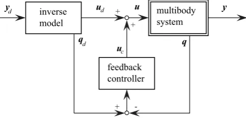
Figure 1.Control structure with feedforward and feedback con-troller.
required in nonlinear control theory. The velocity and accel-eration of the system output follow as
˙y = H(q) ˙q, (4)
¨y = H(q) ¨q+h(q,˙q). (5)
Thereby H∈Rm×f is the Jacobian matrix of the system out-put and h=H ˙q˙ ∈Rm. In trajectory tracking the system out-put (Eq. 3) should track exactly a time-variant outout-put tra-jectory yd(t), which is defined in space and time. Thus also velocity ˙yd(t) and acceleration ¨yd(t) of the system output are
specified.
Multibody systems in output trajectory tracking perform often large working motion. Thus, the equations of mo-tion (Eq. 1) are highly nonlinear and in many instances lin-ear control theory cannot be applied. An efficient approach of output trajectory tracking of nonlinear systems is a so-called two design degree-of-freedom control structure, consisting of a feedforward control and an additional feedback con-trol, see Fig. 1. Thereby the feedforward control is an inverse model of the multibody system. It provides for a given output trajectory yd(t) the associated control inputs ud and the
tra-jectories qdof all generalized coordinates. In the absence of any uncertainties and disturbances the control input udcan be
applied to the multibody system and reproduces the desired output trajectory exactly. Since in a real hardware implemen-tation always some parameter uncertainties and disturbances arise, additional feedback control is necessary and provides additional control input uc. For feedback control design the
computed trajectories qdof the generalized coordinates can
be used as reference signal. In trajectory tracking the most control action is provided by the feedforward part and the feedback part has to compensate only small derivations fol-lowing from uncertainties and disturbances. Therefore, often simple linear control strategies such as PID control might be applicative for the feedback part.
For fully actuated multibody systems, such as fully ac-tuated manipulators, it is f=m. Then, the inverse model
can be derived easily by pure algebraic manipulations, see e.g. Spong et al. (2006). In this case the inverse model can be split into inverse kinematics and inverse dynamics. In inverse
kinematics of a fully actuated system the nonlinear output equation (Eq. 3) can be solved, providing for given yd the trajectories qd of the generalized coordinates. This can be achieved by algebraic manipulations, numerical solution or differential kinematics, respectively. For details it is pointed to Siciliano et al. (2010). By using the determined qd and its derivatives ˙qd,¨qd in the equations of motion (Eq. 1) the
control inputs udcan be computed algebraically.
For underactuated multibody systems the inverse kinemat-ics following from Eq. (3) is under-determined. Also the in-verse dynamics problem cannot be solved since the input ma-trix B is not invertible. Thus, for underactuated multibody systems the splitting of the model inversion into inverse kine-matics and inverse dynamics is in general not possible and both parts must be be solved concurrently. For differentially flat underactuated multibody systems a purely algebraic in-verse model can be derived, using a finite number of deriva-tives of the system output y. In contrast, for non-flat systems the inverse model is a dynamical system. Flatness is a system property determined by the system dynamics and the chosen output, but is independent of the used coordinates to describe the multibody system.
2.2 Servo-constraints in multibody systems
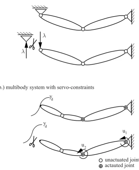
An efficient and straightforward approach for model inver-sion is the use of constraints. The basic idea of servo-constraints is the enforcement of output trajectory tracking by introducing constraint equations. These servo-constraints can be seen as an extension of classical geometric con-straints, which makes this approach so appealing in multi-body system dynamics. In order to introduce the concept of servo-constraints, classical constraints are briefly reviewed. For example, consider a multibody system with a kinematic loop, see Fig. 2. In order to obtain its equation of motion the kinematic loop is cut at a suitable joint, removing n con-straints. Then, the corresponding equations of motion of the open chain system are derived in minimal form and the kine-matic loop is enforced by introducing algebraic loop closing constraints cc(q,t)=0∈Rn. Restricting to a multibody
sys-tem without control action, the equations of motion of the open chain system yields together with the constraint equa-tions,
M(q) ¨q+f (q,˙q)=CTλ, (6)
cc(q)=0. (7)
Thereby C=∂cc/∂q∈Rf×n is the Jacobian matrix of the
y
d
yd
u
u
1
2
unactuated joint actauted joint a.) multibody system with kineamtik loop
b.) multibody system with servo-constraints
Figure 2.Multibody systems with constraints.
In order to derive an inverse model for underactuated multibody systems a similar approach can be used. The prob-lem of tracking a desired trajectory ydis induced by introduc-ing m algebraic servo-constraints. The inverse model of an underactuated multibody systems is then given by the equa-tions motion (Eq. 1) and the servo-constraints,
M(q) ¨q+f (q,˙q)=B(q)u, (8)
c(q,t)=h(q)−yd(t)=0, (9)
where Eq. (9) represents the servo-constraint. As noticed by Blajer (1997a); Blajer and Kolodziejczyk (2004, 2007) the servo-constraint problem Eqs. (8)–(9) is mathematically equivalent to Eqs. (6)–(7). Thereby the desired trajectory
yd(t) can be interpreted as a drift in time of constraint
man-ifold c(q)=0 in the system configuration space, see Bla-jer (2001). The generalized actuating forces Bu can then be viewed as a generalized reaction forces of the servo con-straints. Thus, structurally the generalized actuation forces
Bu corresponds to the generalized reaction forces CTλ.
Therefore, in the servo-constraint approach the control inputs
u ensure that the servo-constraints are met. The similarities
between both cases are illustrated in Fig. 2.
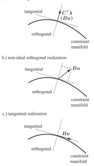
At first, multibody systems with servo- and physical con-straints show many similarities. However, servo-constraint problems can posses more complex properties, which have to be understood to obtain a meaningful solution. For a
multi-body system with classical constraints the matrix CTprojects the Lagrange multipliersλon the directions orthogonal to the constraint manifold, which is defined by the constraint equa-tion (Eq. 7). Thus, the generalized reacequa-tion forces CTλare orthogonal to the constraint manifold, see Fig. 3. Therefore such a system is called an ideal orthogonal realization.
In contrast, the generalized actuation forces Bu are not necessarily ideal orthogonal to the constraint manifold which is defined by the servo-constraint (Eq. 9). The actuation forces Bu might be non-ideal orthogonal or in the extreme case even tangential to the constraint manifold, see Fig. 3. These cases are called non-ideal orthogonal realization and tangential realization, respectively. Thereby, ideal and non-ideal orthogonal realization have many similarities, and are in the following only distinguished, if different phenomena occur. In the case of both types of orthogonal realization con-trol inputs are explicitly available in all directions orthogonal to the constraints and can directly actuate the servo-constraint condition. However, in the case of non-ideal or-thogonal realization the projection with B yields also compo-nents in direction tangential to the constraint manifold. In a tangential realization the control inputs are projected in tan-gential direction. Then, the control inputs u cannot actuate directly the constraint condition, but output tracking of yd might be still possible due to coupling with other forces of the system, see Blajer and Kolodziejczyk (2004). This tan-gential projection is often connected to underactuated diff er-entially flat systems. However, as will be shown in section 3 tangential realization can also arise in non-flat systems. Fur-ther analysis from a geometric point of view are also found in Blajer (1992), Blajer and Kolodziejczyk (2004) and Blajer and Kolodziejczyk (2007).
For systems with multiple inputs and outputs it might oc-cur that both, orthogonal (ideal or non-ideal) and tangen-tial realization exist. Thus, in so-called mixed orthogonal-tangential realizations only some outputs can be directly in-fluenced by the inputs, while others can only be inin-fluenced indirectly. A measure of the control singularity is the defi-ciency in rank p of the matrix
P=H M−1B. (10)
The case p=m indicates that all components of the system
output y can directly be actuated by the inputs u. The case 0<p<m shows that only p components of the output can be
regulated in the orthogonal way, while realization of the other
m−p output components are without direct involvement of
the actuating forces Bu. Finally, p=0 refers to a pure tan-gential realization of servo-constraints, as the system inputs do not directly influence the outputs.
If the solution of the servo constraint problem (Eqs. 8–9) exists, the numerical solution of this DAE provides the trajec-tories of all states qd,˙qdas well as the corresponding control
inputs ud. For characterizing DAEs often the differentiation
b.) non-ideal orthogonal realization
c.) tangential realization a.) ideal orthogonal realization
( )
orthogonal tangential
constraint manifold
constraint manifold
constraint manifold orthogonal
tangential
orthogonal tangential
Figure 3.Possible realizations in servo-constraint problems.
or parts of it, until an ordinary differential equation (ODE) for all unknowns are obtained. For multibody systems with classical constraints it is well know that they have diff eren-tiation index 3. Here the constraint equation (Eq. 7) must be differentiated three times in order to derive an ODE for the unknownλ. This is provided by the fact that for classical con-straints the matrix (Eq. 10) becomes P=C M−1CT, which has full rank if the constraints are independent, see Hairer and Wanner (2010).
In the case of servo-constraints this is not any more nec-essarily true. In the case of orthogonal realizations P has full rank and index 3 arises. However, if the servo-constraint problem includes a tangential realization P is singular and higher differentiation index arise. For various mechanical systems with servo-constraints the differentiation index is an-alyzed in Campbell (1995).
The differentiation index is closely related to the relative degree used in differential geometric nonlinear control the-ory. An extensive treatment of this nonlinear control theory is given in Isidori (1995); Sastry (1999). Restricting to sys-tems with n states and one input and one output, the relative degree r is the number of Lie derivatives of the system output
until the first time the control input occurs. If the relative de-gree is r=n, then the system is differentially flat and a purely algebraic inverse model can be extracted. In the case r<n
so-called internal dynamics remain and the inverse model will contain a dynamical part. For extension to systems with mul-tiple inputs and outputs it is pointed to the aforementioned nonlinear control literature. In Campbell (1995) it is pointed out that the differentiation index is one higher than the rel-ative degree, if the internal dynamics are not affected by a constraint.
2.3 Projection approach
In Blajer (1997a) it is shown that the equation of motion with additional constraints can be projected into two complemen-tary subspaces in velocity space. These are the constrained and unconstrained subspace. The unconstrained subspace is tangential to the constraint manifold, while the constrained subspace is orthogonal to it, see Fig. 3. The constrained sub-space describes in the servo-constraint context the output subspace and follows from projection with the Jacobian ma-trix H∈Rm×fof the output, which has rank m. For the second
subspace an orthogonal complement D∈Rf×f−mwith rank
f−m must be derived, such that
H D=0 and DTHT=0 (11)
is satisfied. Using these two matrices the equations of motion are projected into the two subspaces,
h H M−1 DT
i
M ¨q+f−Bu=0, (12)
which yields,
H ¨q+H M−1f=H M−1Bu, (13)
DTM ¨q+DTf=DTBu. (14)
With the output equation (Eq. 5) at acceleration level the cor-responding servo-constraint provides H ¨q=¨yd−h. This
rela-tionship can be used in Eq. (13). Introducing the new state
v=˙q and adding the servo-constraints at position level, after reordering the projected servo-constraint formulation, pro-vides
˙q = v (15)
DTM˙v = −DTf+DTBu (16)
0 = Pu−H M−1f+h−¨yd (17)
0 = h(q)−yd. (18)
This forms a set of 2 f+m differential-algebraic equations for the 2 f+m unknowns q,v,u. Equation (17) has dimension m
and describes an algebraic equation in q,v,u. Together with
two is achieved, which in general simplifies the numerical solution. For example, for the crane considered in Blajer and Kolodziejczyk (2004, 2007), the differentiation index is re-duced from 5 to 3 using this projection approach.
2.4 Coordinate transformation
The numerical solution of Eqs. (15)–(18) provides the model inversion. However, for analysis purpose it might be of ad-vantage to write first the equations of motion in a new set of coordinates containing the system output. In addition, this might also be used to simplify the projections in Eqs. (15)– (18). Also for systems with orthogonal realization an inverse model as ODE can be derived in a straightforward way. For example, as new set of coordinates
q=h y
qu i
=h h(qa,qu) qu
i
=φ(q) (19)
might be used, which yields for the velocities
˙q=h ˙y
˙qu i
=h Ha Hu
0 I
ih ˙qa
˙qu i
=∂φ(q)∂
q ˙q. (20)
It is noted that the first row of Eq. (20) is identical to Eq. (4), i.e. H=[Ha Hu]. In order to be an admissible coordinate
transformation, it must be a diffeomorphism, i.e. smooth and invertible. Relationship (Eq. 19) is at least a local diff eomor-phism if the Jacobian matrix in Eq. (19) is non-singular. In-specting Eq. (19) shows, that this is true if the submatrix Ha
is nonsingular. This requires that the output equation (Eq. 3) depends on all m actuated coordinates qa. This is for example
the case for manipulators with flexible links or passive joints in end-effector tracking. A counterexample is a manipulator with flexible joints in end-effector tracking, see e.g. De Luca (1998).
With the results of Eq. (5) the coordinate transforma-tion (Eq. 19) at acceleratransforma-tion level is,
¨q=h ¨y
¨qu i
=h Ha Hu
0 I
ih ¨qa
¨qu i
+h h
0
i
. (21)
From the equations of motion (Eq. 1) follows ¨q=M−1(Bu− f ) which can be inserted in Eq. (21) and yields
¨y = Pu−H M−1f+h, (22)
¨qu =
0 ... IM−1(Bu−f ). (23)
In all entries of these two equations the original states qa,˙qa
must be replaced by the new states y,˙y. Therefore the upper part of Eq. (19) must be solved for qa, which is in general nonlinear. Afterwards the velocities ˙qacan be computed from the linear equations provided by Eq. (20).
The two second order differential Eqs. (22)–(23) represent the equations of motion of the multibody system expressed in the new coordinates q, which include the system output y.
The equations of motion (Eqs. 22–23) can be helpful in ana-lyzing both, orthogonal and tangential realization, as will be seen in the next subsection.
The coordinate transformation approach is inspired by differential-geometric control theory, which is the basis of feedback linearization and can also be used for feedforward control design, see Isidori (1995); Sastry (1999). Thereby, nonlinear systems are transformed by diffeomorphic coor-dinate transformations into the so-called nonlinear input-output normal form using new states, containing the input-output and a finite number of its time derivatives. The application of this nonlinear control theory to underactuated multibody sys-tems in orthogonal realization is given in Seifried (2012a,b). The following short discussion highlights some correspon-dence of the servo-constraint approach with aforementioned nonlinear control theory for underactuated multibody sys-tems in orthogonal realization. In this case, the equations of motion (Eqs. 22–23) in new coordinates q are identi-cal to the nonlinear input-output normal form. The matrix
P=H M−1B is called decoupling matrix in nonlinear control
theory. Equation (22) links the input u to the second deriva-tive of the output ¨y, describing the input-output relationship. Equation (23) is called in nonlinear control theory the inter-nal dynamics. This is the remaining system dynamics of the inverse model. From this input-output normal form feedback linearization and feedforward control design are easily pos-sible. For a desired output trajectory ydthe necessary control
input follows from Eq. (22) as
ud=P−1(H M−1f−h+¨yd). (24)
It is noticed that this is structurally identical to Eq. (17), however expressed in terms of the new coordinates. Equa-tion (24) is an algebraic expression for the input, depending solely on the known values yd,˙yd and the unknowns qu,˙qu.
The later ones follow from solving the internal dynamics by applying Eq. (24) to the ODE Eq. (23), resulting in
¨qu = 0 ... IM−1[BP−1(H M−1f−h+¨yd)−f ],
= a(qu,˙qu,yd,˙yd,¨yd). (25)
These are f−m second order differential equations for qu, driven by the desired output ydand its derivatives ˙yd,¨yd.
3 Illustrative example 1: mass on car
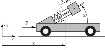
The different phenomena which might arise in servo-constraint problems of underactuated multibody systems are demonstrated using a spring-mass system mounted on a car, which is shown in Fig. 4. The car with mass m1moves along
the horizontal e1axis and is actuated by the force u=F. On
the car a mass m2 is mounted, which moves along an axis
which is inclined by the angleα. The system is described by the two generalized coordinates q=[x,s], whereby x is
x F
s
α
Figure 4.Mass on car system.
mass along the inclined axis. Thereby, qa=x is the
actu-ated coordinate and qu=s is the unactuated coordinate. The
mass is supported by a parallel spring-damper combination, with spring and damping coefficients k,d, respectively. In the
equilibrium position it is s=0. This yields the equations of motion
"
m1+m2 m2cosα
m2cosα m2 # "
¨x ¨s
# +
"
0
ks+d ˙s #
= "
F
0
#
. (26)
The system output is the horizontal position of the mass,
y=x+s cosα, (27)
which should follow a predefined trajectory yd(t). This yields
the servo constraint
c(q,t)=x+s cosα−yd(t). (28)
Equations (26) and (28) form the servo-constrained problem. From Eq. (28) follow the two projection matrices,
H=h 1 cosα i, D=
"
cosα
−1
#
. (29)
With these matrices the projected Eqs. (15)–(18) of the servo-constraint problem can be computed. Thereby it follows from Eq. (18)
P=H M−1B= sin 2α
m1+m2sin2α
. (30)
It becomes apparent that this matrix is nonsingular forα,0,
i.e. it poses an orthogonal realization. However forα=0 a tangential realization occurs.
In order to analyze this servo-constraint problem in more detail, the coordinate transformation approach presented in Sect. 2.4 is applied. The new set of coordinates contain-ing the output are chosen as q=[y,s]. The system dynamics
in new coordinates follows from evaluating Eqs. (22)–(23),
¨y=−m1cosα[ks+d ˙s] m1m2+m2
2sin 2α+
sin2α
m1+m2sin2αF, (31)
¨s=−(m1+m2)[ks+d ˙s] m1m2+m22sin
2α −
cosα
m1+m2sin2α
F. (32)
Based on this description of the system dynamics different occurring phenomena are discussed, whereby four different cases are distinct.
Case 1: the relative motion of the mass occurs in vertical di-rection, i.e.α=90◦, see Fig 5a. In this case the system output
is identical to the car position y=x and (Eq. 30) reduces to P=(m1+m2)−1,0. Thus, the equations of motion Eq. (26)
and Eqs. (31)–(32) coincide and provide
(m1+m2)¨y = F (33)
m2¨s = −ks−d ˙s. (34)
Both equations are here fully decoupled. The force F is orthogonal to the constraint manifold, which is described by the servo-constraint (Eq. 28), see Fig. 5a. This is identical to classical geometric constraints and the control force regulates directly the output. The control action which is necessary to reproduce the output trajectory follows from Eq. (33) as Fd=(m1+m2)¨yd. The dynamics of the
mass in vertical direction is described by Eq. (34) and is not influenced by the control force and vice versa. This dynamics of the mass cannot be observed by the system output y and thus in reference to nonlinear control theory this dynamics (Eq. 34) is called internal dynamics, see Isidori (1995) and Sastry (1999).
Case 2: the mass moves along a tilted slope with
0◦< α <90◦, see Fig. 5b. The system dynamics in new
coordinates are given by Eqs. (31)–(32) and from Eq. (30) follows P,0. This indicates a non-ideal orthogonal real-ization since the control force has an orthogonal component to the constraint manifold. The control force F can still regulate directly the constraint condition, however it also has a component in tangential direction influencing the relative motion of the mass, see Fig. 5b.
For a given output trajectory yd Eq. (31) can be solved
algebraically for the desired control input,
Fd=
m1+m2sin2α sin2α ¨yd+
m1cosα[ks+d ˙s]
m2sin2α . (35)
The control input depends on the second derivative of the system output ¨ydand the unknown states s,˙s which must be
computed from Eq. (32). Replacing in Eq. (32) the control input by Eq. (35) yields after reordering
m2sin2α¨s+d ˙s+ks=−¨ydm2cosα. (36)
This is the dynamics of the mass m2 on the tilted slope
y F
constraint manifold
F
y F
constraint manifold
F
constraint manifold
F ideal orthogonal realization (index 3, non-flat)
non-ideal orthogonal realization (index 3, non-flat)
tangential realization
a.) case 1 b.) case 2
c.) case 3 and 4
case 3: with damping: index 4 (non-flat)
case 4: without damping: index 5 (differentially flat) x
s
yd x
s
yd
y
F yd x, s
Figure 5.Possible situations arising in servo-constraint problems.
the internal dynamics is a second order differential equation, which is driven by the second derivative of the desired system output trajectory yd.
Case 3: the mass moves in horizontal direction, i.e. α=0◦, see Fig. 5c. For this case the equations of motion in
new coordinate follow from Eqs. (31)–(32) after reordering as
m2¨y=−ks−d ˙s, (37)
m1m2¨s=−(m1+m2)[ks+d ˙s]−m2F. (38)
In addition, it follows from Eq. (30) that P=0. This indicates a tangential realization, where the control force F is tangen-tial to the constraint manifold, see Fig. 5c. Thus F cannot directly regulate the servo-constraint, i.e. the system output
y. This is also seen from Eq. (37), which contains ¨y, but not
any more the control input F. However, output tracking of y is still possible due to coupling with other forces of the sys-tem, here the spring force and damper force.
For tracking of the desired output trajectory yd, the
neces-sary control input can be computed form Eq. (38) as
Fd=−
(m1+m2)
m2 [ks+d ˙s]−m1¨s. (39)
Firstly, the values of s,˙s,¨s are unknown. For given ydthese
can be computed from Eq. (37) as,
ks+d ˙s=−m2¨yd. (40)
This is a differential equation for s and poses in this case the internal dynamics. In contrast to the previous two cases, the internal dynamics is here a first order differential equation. For given ¨yd the solution of the internal dynamics Eq. (40)
provides the corresponding values sd. Then, the values ˙sd
fol-low directly form the algebraic solution of Eq. (40) as
˙sd=− ksd
d − m2
d ¨yd. (41)
Taking one time-derivative of Eq. (41) yields an algebraic expression for ¨sd,
¨sd=− k d˙sd−
m2 d y
(III)
d . (42)
Thus, all quantities for evaluating the control force F using Eq. (39) are available. The last equation shows, that in contrast to the previous two cases the third derivative of the desired output trajectory ydmust be available.
Case 4: the mass moves in horizontal direction and no damping is present, i.e. α=0◦ and d=0. Similar to case
3 a tangential realization exists since P=0, and the same interpretations apply. The equations of motion in new coordinates simplifies to
m2¨y=−ks, (43)
m1m2¨s=−(m1+m2)ks−m2F. (44)
Similarly to case 3, the control force Fdcan be computed
al-gebraically form Eq. (44), where s,¨s are unknowns. In con-trast to case 3 Eq. (43) is now an algebraic expression for computing sdfor given ¨yd,
sd=− m2
k ¨yd. (45)
Taking two time-derivatives of Eq. (45) yields
¨sd=− m2
k y (IV)
The last equation shows, that in this case the forth derivative of the output trajectory is necessary. Combing Eqs. (44)–(46) yields the control force
Fd=(m1+m2)¨yd+ m1m2
k y (IV)
d . (47)
Thus, in this case the control input ud and all states yd,˙yd,sd,˙sd of the system can be computed by purely
algebraic manipulations, without the need of solving any differential equations. Thus, since all these quantities are specified by the system output y and its four time-derivatives, this case poses a differentially flat system.
Summary and comparison of cases: the servo-constraint problem for this illustrative example has been analyzed using the coordinate transformation approach. Of course, also the DAEs (Eqs. 8–9) or the projected DAEs (Eqs. 15–18) can be established. Thereby, the previous analysis can be used to analyze the differentiation index. In accordance with the discussion at the end of Sect. 2.2 it can be obtained that the differentiation index of the original DAEs (Eqs. 8–9) is one higher than the highest derivative of the system output y which is necessary to compute the control force F.
The cases 1 and 2 are orthogonal realizations and therefore provide DAEs with differentiation index 3, similar to systems with geometric constraints. This is irrespectively of the exis-tence of damping in the system. The dynamics along the con-straint manifold is not specified by the output, which forms the internal dynamics. Thus, these are two differentially non-flat mechanical systems. These cases 3 and 4, with tangential realizations, yield higher differentiation index, which is de-pendent on the existence of damping. In case 3, where damp-ing is present, the system has index 4. Internal dynamics re-main, which in this case is a dynamical system of first order. Thus this example with damping poses a tangential realiza-tion for a differentially non-flat system. In case 4 no damping exists and differentiation index 5 arises. Then, the complete motion is specified by the trajectory of the output y and its time-derivatives. No internal dynamics remains and this tan-gential realization represents the case of a differentially flat underactuated mechanical system. It should be mentioned, that differentially flat systems with higher index exist. Such an example is the n-mass-spring chain as analyzed in Blajer (1997b).
This example is representative for the different possible phenomena in servo-constraint problems of underactuated multibody systems. An orthogonal realization yields index 3 and internal dynamics remains, which are described by f−m
differential equations of second order. For tangential realiza-tion higher index arise. Thereby an increasing differentiation index indicates a reduced size of the internal dynamics and the need for higher derivatives of the output trajectory. In the limit cases no internal dynamics remains, and the system can be inverted purely algebraically, i.e. the system is diff eren-tially flat.
4 Stability of the internal dynamics
The previous discussion highlights that the inverse model might be a dynamical system, namely containing internal dy-namics. This can occur in both cases, the orthogonal real-ization and the tangential realreal-ization. In the computation of the inverse model these internal dynamics must be solved. Thereby, the stability of the internal dynamics, i.e. the sys-tem dynamics of the servo-constraint problem, must be in-vestigated carefully. For an ideal orthogonal realization, e.g. classical constraints, the stability properties and analysis of multibody systems with classical constraints applies. This ideal orthogonal realization also occurs in underactuated multibody systems with collocated inputs and outputs, i.e. there is a control input at each system output. This occurs for example in case 1 of the mass on car example which is presented in Sect. 3.
For non-ideal orthogonal and tangential realization, the in-ternal dynamics might be more complex, and stability might not be ensured. This is due to the combination of the multi-body system with a control, whereby inputs and outputs are not collocated. In the case of unstable internal dynamics, for-ward time integration of the internal dynamics might yield unbounded states and control inputs, which provides an un-feasible inverse model. Therefore, careful stability analysis of the internal dynamics is necessary. Using the coordinate transformation approach the internal dynamics of the inverse model can be extracted explicitly, which is helpful in system analysis. For example, for the orthogonal realization the in-ternal dynamics is given by Eq. (25).
In general, the internal dynamics is nonlinear and driven by the desired output trajectory yd(t), posing a nonlinear time-variant system. Since stability analysis of such systems is quite complex, one uses often the concept of zero dy-namics, see Isidori (1995); Sastry (1999). The zero dynam-ics is the internal dynamdynam-ics under a constant system out-put, e.g. yd=0,∀t. This reduces the internal dynamics to a
time-invariant nonlinear system. For the orthogonal realiza-tion follows from Eq. (25) the zero dynamics,
¨qu=a(qu,˙qu). (48)
Local stability of the zero dynamics can then be checked, e.g. using Lyapunov’s indirect method. Local asymptotic sta-bility requires that the linearized zero dynamics has only eigenvalues with negative real part. If at least one eigenvalue has a positive real part the system is unstable. If there are both, eigenvalues with negative real part and purely imagi-nary eigenvalues, then Lyapunov’s indirect method is incon-clusive. In this case stability can be checked e.g. using Lya-punov’s direct method, see e.g. Khalil (2002), or the center manifold method, see e.g. Isidori (1995).
−15 −10 −5 0 −10
−5 0 5 10
Real(λ)
Imag(
λ
)
α=90°
α=9.1°
λ1, λ2, d=1Ns/m
λ1, λ2, d=0Ns/m
0° α α 0°
α
0
°
0
°
α
Figure 6.Eigenvalues of zero dynamics for mass on car system.
nonlinear systems and zeros of linear systems are discussed in Isidori and Moog (1988). A linear system is called min-imum phase, if all its zeros are in the open left half plane, i.e. its zero dynamics is exponentially stable. This defini-tion is also extended to nonlinear systems. In nonlinear con-trol theory systems with asymptotical stable zero dynamics are called asymptotically minimum phase, otherwise non-minimum phase, see Isidori (1995). It is important to no-tice, that local asymptotic stability of the zero dynamics is a necessary but not sufficient condition for stability of the driven internal dynamics. This last step is often very com-plex and from a practical point one restricts often to verify local asymptotic stability of the zero dynamics.
4.1 Illustrative example 1: stability of mass on car
For the mass on car example in Sect. 3 internal dynamics remains for cases 1–3. Figure 6 shows the location of the eigenvalues of the zero dynamics for 0◦≤α≤90◦, i.e. case 1
and 2. The system properties are summarized in Table 1. The eigenvalues of the zero dynamics follow from the internal dynamics (Eq. 36) with ¨yd=0. The internal dynamics is in
these cases similar to a spring-mass system and is therefore asymptotically stable for the damped case and stable for the undamped case. Forα=90◦ it is identical to a free damped mass-spring system and mass m2 vibrates freely in vertical
direction. Hereby, in the undamped case the eigenfrequency of the free vibration isω=0.25 Hz. However, with the incli-nation angleαthe dynamic behavior of the internal dynamics changes. Thus for example, forα=5◦and d=0 Ns m−1 the
eigenfrequency of the zero dynamics increases to 2.88 Hz. Also in the damped case the behavior changes dramatically, and forα <9.1◦ and d=1 Ns m−1an over-damped behavior
occurs. Thus, due to the servo-constraint, the dynamical be-havior of the internal dynamics can be quite different from the dynamics of the uncontrolled underactuated multibody system.
Table 1.Properties for mass on car system.
m1=1 kg m2=2 kg k=5 N m−1 d=0 Ns m−1and d=1 Ns m−1
S
y s
c
d T
α
β
Figure 7.Rotational arm with passive joint.
4.2 Illustrative example 2: rotational manipulator arm
As simple example for an underactuated multibody system with unstable internal dynamics a single rotational manipu-lator arm with a passive joint is considered, see Fig. 7. The rotational arm consists of two identical homogenous links with length l, center of mass s=l/2, mass m and inertia
I=ml2/12. The first link is actuated by the control torque u=T . The second link is connected by a passive joint to
the first link, which is supported by a linear spring-damper combination with spring constant c and damper coefficient
d. Thus, the passive joint manipulator has its elasticity
par-allel to the joint and shows very many similar properties as manipulators with flexible links, see Seifried et al. (2013). In contrast, such a passive joint system is quite different to a so-called flexible joint manipulator with drive train elas-ticities, where the flexibility is located between a link of the manipulator and its motor, see De Luca (1998).
The rotational manipulator arm is described by the gen-eralized coordinates q=[α, β], whereby qu=βdenotes the
unactuated coordinate. The arm moves perpendicular to the direction of gravity and the equations of motion are given by
l2m " 5
3+cosβ 1 3+
1 2cosβ 1
3+ 1 2cosβ
1 3
# "
¨
α
¨
β #
+
"
−0,5l2m ˙β(2 ˙α+β˙) sinβ
cβ+d ˙β+0,5l2m ˙α2sinβ
# =
" T
0
#
. (49)
The position of a point S on the second link is described in the body fixed coordinate system by 0<s<l, see Fig. 7.
The control goal is the tracking of the position of point S . For smallβthe position can be described approximately by the system output
y=α+ s
s+lβ. (50)
see Fig. 7. For example, with this auxiliary angle the position in e2direction is
rs2=l sinα+s sin(α+β)≈(l+s) sin y. (51)
This approximation holds for small β, which can be veri-fied by computing the Jacobian linearization aroundβ=0, see Seifried (2012b). It is noted, that the following computa-tions and analysis for the exact position of S follow the same steps and yield the same results. However, the use of the lin-early combined system output (Eq. 50) simplifies the expres-sions significantly and allows an easier discussion of the re-sults. Similar linearly combined outputs are also often used in end-effector tracking of flexible manipulators, see e.g. De Luca (1998); Seifried et al. (2011).
For this rotational arm the servo-constraint is given by
c(q,t)=α+ s
s+lβ−yd(t) (52)
and its Jacobian matrix is
H=h 1 l+ss i. (53)
With this matrix follows from Eq. (18)
P=H M−1B= 2l(3s cosβ−2l)
ml2(l+s)(9 cos(2β)−23). (54)
For s∗=2l/(3 cosβ) it is P=0, i.e. only for this cases a
tan-gential realization occurs. For small anglesβthe position s∗
approximates the center of percussion. In Fliess et al. (1995) it is shown, that for a manipulator with one passive joint the center of percussion might yield a differentially flat system output. In contrast, in the following the case s,s∗is
consid-ered, i.e. the case of an orthogonal realization. If s=0 then the input and output are collocated since y=α. In this case an ideal orthogonal realization occurs, otherwise a non-ideal orthogonal realization exists. From the previous discussions it is obvious that internal dynamics remain.
To analyze the internal dynamics and the servo-constraint problem in more detail, the coordinate transformation ap-proach presented in Sect. 2.4 is applied. The new set of co-ordinates containing the output are chosen as q=[y, β]. The system dynamics in new coordinates follows from evaluating Eqs. (22)–(23). For a given output trajectory yd the required
control input udfollows from Eq. (24). Then, the system
dy-namics of the inverse model, i.e. the internal dydy-namics, are described by Eq. (25). For its analysis the zero dynamics is derived, which follows from the internal dynamics with
y=0,∀t. For this example the zero dynamics turns out to be ml2(s+l)(2l−3s cosβ) ¨β
=−3ms2l2sinββ˙2−6(s+l)2(cβ+d ˙β). (55)
For analysis the zero dynamics (Eq. 55) is linearized around its equilibrium pointβ=0 yielding
ml2(2l−3s)
| {z } a2
¨˜
β+6d(s+l)
| {z } a1
˜
β+6c(s+l)
| {z } a0
˙˜
β=0. (56)
Table 2.Properties for rotational manipulator arm.
l=1 m m=3.438 kg k=50 Nm rad−1 d=0.25 Nms rad−1
−100 −50 0 50 100
−100 −50 0 50 100
Real(λ)
Imag(
λ
)
s/l=0 s/l=1
s/l → 2/3
s/l → 2/3
s/l → 2/3 2/3 ← s/l
λ1 λ2
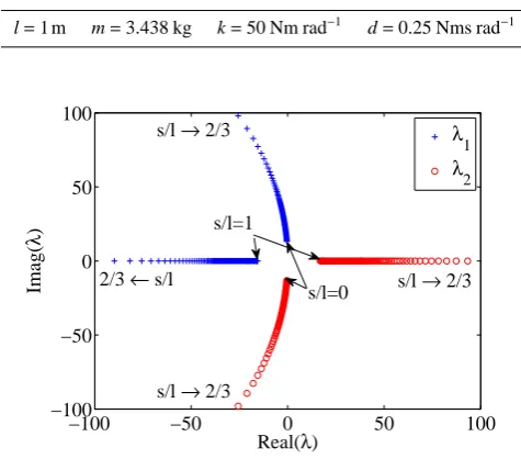
Figure 8.Eigenvalues of zero dynamics for rotational arm.
Thereby a2,a1,a0 correspond to the coefficients of the
char-acteristic polynomial. Using Stodola’s criterion the lin-earized zero dynamics (Eq. 56) of the rotational arm is only asymptotically stable, if all coefficients a2,a1,a0 have the
same sign and are non-zero. The constants c,d of the
spring-damper combination and the dimensions l,s are by nature
positive, yielding positive constants a0,a1. Thus also the
co-efficient a2must be positive to obtain stable internal
dynam-ics. From this follows that for s/l<2/3 the internal dynamics is locally asymptotically stable, while for s/l>2/3 the in-ternal dynamics is unstable. The location of the eigenvalues for different 0≤s≤1 is shown in Fig. 8. The used system parameters are summarized in Table 2. This shows clearly that the dynamics of a servo-constraint problem, namely its internal dynamics, might be fundamentally different from the dynamics of the uncontrolled mechanical system. End-effector tracking, i.e. s=l, is in robotic manipulator
applica-tions the most interesting case. The presented analysis shows that in this example unstable internal dynamics occur in end-effector trajectory tracking.
The analysis of the rotational arm shows that the stability of the internal dynamics can depend on the choice of the sys-tem output location. In addition, if a non-homogenous design for the links is admitted, the stability of the internal dynam-ics also depends on the mass distribution of the links, see the analysis in Seifried (2012b). Then, the mass distribution can also be designed in such a way that for end-effector trajectory tracking stable internal dynamics remain.
such systems are given e.g. in Seifried (2012b) and Seifried et al. (2011), respectively.
5 Numerical solution
In most cases the inverse model requires a numerical so-lution, whereby the solution method depends on the previ-ously analyzed system properties. In the following some ba-sic numerical solution methods are summarized for diff eren-tially flat systems, systems with stable internal dynamics and systems with unstable internal dynamics. For demonstration purpose these methods are applied to the two presented illus-trative examples. The following presentation highlights some solution issues and demonstrates also the effect of the diff er-ent system properties. However, it is not meant as a full in depth investigation of numerical time integrators for servo-constraint problems.
5.1 Differentially flat systems
For differentially flat systems, a purely algebraic inverse model can be derived. However, this requires often a large number of symbolic time-derivations and manipulations of the output equation and the equations of motion. This might be possible for small systems, such as in case 4 of the mass on car system, but for larger systems these symbolic compu-tations might become very burdensome. Therefore, also for differentially flat systems a numerical solution based on the servo-constraint approach might be useful.
Due to the tangential realization in underactuated diff er-entially flat systems the original servo-constraint formula-tion (Eqs. 8–9) has differentiation index greater 3. For the numerical solution the use of the projection approach pre-sented in Sect. 2.3 might be advantageous, yielding a index reduction. Then, the set of differential-algebraic Eqs. (15)– (18) must be solved numerically. For readability these equa-tions are summarized as
˙q = v (57)
A˙v = a(v,q,u) (58)
0 = b(v,q,u,¨yd) (59)
0 = c(q,yd). (60)
The solution of this set of 2 f+m equations are variations
in time of the m control inputs u(t) which are required for the exact reproduction of the desired output trajectory yd(t), and variations of the 2 f states q(t),v(t)=˙q(t) in the specified motion.
Since differentially flat systems can completely be inverted algebraically, the output specifies completely the entire mo-tion of the system and Eqs. (57)–(60) do not contain any in-ternal dynamics. This allows the efficient use of rather simple solution formulas. A simple numerical solution schema for solving the DAEs can be based on the Euler backward diff er-entiation scheme, as proposed by Blajer and Kolodziejczyk
0 2 4 6 8 10
0 0.5 1 1.5 2 2.5 3
time [s]
desired trajectory y
d
[m]
Figure 9.Desired output trajectory ydfor mass m2.
(2004). Thereby the time derivatives ˙q and ˙v are approx-imated with their backward differences (qn+1−qn)/∆t and
(vn+1−vn)/∆t, respectively. Thereby∆t is the constant
inte-gration time step, such that tn+1=tn+ ∆t. With the known
values qn,vn at time tn, the solution qn+1,vn+1,un+1 at time tn+1can be obtained from the solution to the set of nonlinear
algebraic equations
qn+1−qn−∆tvn+1 = 0 (61)
A(qn+1)[vn+1−vn]−∆ta(vn+1,qn+1,un+1) = 0 (62) b(vn+1,qn+1,un+1,¨yd,n+1) = 0 (63)
c(qn+1,yd,n+1) = 0. (64)
This schema can also be used for systems with mixed ge-ometric and servo-constraints as presented in Blajer and Kolodziejczyk (2011).
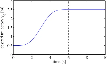
This very basic solution schema is applied to the mass on car system. Mass 2 should follow the output trajectory
yd=y0 + h
126( t
tf−t0)
5−420( t tf−t0)
6+540( t tf−t0)
7
− 315( t
tf−t0)
8+70( t tf−t0)
9i
(yf−y0), (65)
whereby starting point y0=0.5 m and finial point yf =2.5 m
are chosen. After reaching the final point at time tf =6 s
the output is at rest. The complete simulation time is 10 s. This trajectory is designed in such a way, that also its higher derivatives are sufficiently smooth. The trajectory is shown in Fig. 9.
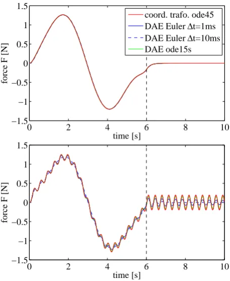
It is noticed that the original servo-constraint problem has differentiation index 5, while the projection approach yields index 3. Figure 10 shows the control forces ud computed
with the projection approach and compared to the analytical solution from Eq. (47). This shows, that this rough compu-tational scheme is of acceptable accuracy for appropriately small values of∆t. Here, the Euler backward schema yields
0 2 4 6 8 10 −1
−0.5 0 0.5 1 1.5 2
time [s]
force F [N]
analytic Euler Δt=1ms EulerΔ t=10ms EulerΔ t=100ms Radau
Figure 10.Mass on car – case 4, flat system: computed control input ud.
completly specified by the output. Thus, it can be argued that in this case the issue of numerical damping, which for such a simple discretization schema normally appears, might not pose a significant problem here.
More accurate time discretization schema can be used for the solution of the servo-constraint problem of differentially flat underactuated multibody systems. Therefore, in Fig. 10 also the solution obtained by a Radau IIa schema is added. This method is capable of handling index 3 DAEs, see Hairer and Wanner (2010). Hereby an accurate solution is obtained by using only 56 time points. This compares to 1000–10 000 points using the Euler backward schema. In literature fur-ther solution methods have been proposed for differentially flat servo-constraint problems. Betsch et al. (2007, 2008) use a energy conserving schema for solving the projected Eqs. (57)–(60), whereby redundant coordinates are used. For a differentially flat crane Fumagalli et al. (2011) propose a solution based on backward differentiation formula.
In Fig. 11 the analytical solution for the desired trajectories of the generalized coordinates and its derivatives are shown. Since hardly any differences to the numerical solutions are visible, the presentation of the numerical solutions are omit-ted here. From Fig. 11, as well as from the control force plot, it is seen that the complete system is at rest after tf=6 s,
indi-cating the final position of the output. This is due to the fact that for this system the output trajectory specifies the com-plete system behavior and no internal dynamics remain. This is typical for a differentially flat system.
5.2 Systems with stable internal dynamics
Underactuated multibody systems with stable internal dy-namics can be solved by forward time integration. There-fore, the same numerical integrators as in the previous dis-cussed differentially flat case might be used. This is demon-strated using the mass on car system with an inclination an-gle ofα=5◦, representing a non-ideal orthogonal
realiza-0 2 4 6 8 10
−1 0 1 2 3
time [s]
position x [m]
x s
0 2 4 6 8 10
−0.2 0 0.2 0.4 0.6
time [s]
velocity [m/s]
Figure 11. Mass on car – case 4, flat system: computed states
qd,˙qd.
tion. Thereby the case of a strongly damped system with
d=1 Ns m−1and the undamped system are considered. By using the projection approach, index 1 DAEs arise for the orthogonal realization. As numerical solution schema for the projected servo-constraint Eqs. (15)–(18) the previously presented Euler backward schema with time step size 1ms and 10 ms are used. In addition a numerical backward dif-ferentiation formula is used, as implemented in the Matlab function ode15s, see Shampine et al. (1999). This is capa-ble of solving index 1 DAEs. Also the coordinate transfor-mation approach is used. Hereby the internal dynamics is given explicitly by Eq. (36) and the control input follows from Eq. (35). For the numerical solution of the internal dy-namics (Eq. 36) the Matlab ode45 integrator is used, which is an explicit Runge-Kutta formula of order 4 and 5 using the Dormand-Prince pair.
The obtained control forces using the different solution methods are shown for the damped and undamped case in Fig. 12. The velocities of the generalized coordinates are presented in Fig. 13. Since differences between the solution methods are seen best in the control force, the velocity plot shows only the solution obtained using the coordinate trans-formation approach.
0 2 4 6 8 10 −1.5
−1 −0.5 0 0.5 1 1.5
time [s]
force F [N]
coord. trafo. ode45 DAE Euler Δt=1ms DAE Euler Δt=10ms DAE ode15s
0 2 4 6 8 10
−1.5 −1 −0.5 0 0.5 1 1.5
time [s]
force F [N]
Figure 12.Mass on car – case 2,α=5◦
: computed control input ud.
With damping d=1 Ns m−1(top) and without damping (bottom).
seen from the force and velocity plots. The remaining mo-tion of the system is its zero dynamics. For the case with
d=1 Ns m−1 an overdamped internal dynamics occurs, as also seen from the eigenvalue plot of the zero dynamics in Fig. 6. Thus, the internal dynamics decays rapidly. In con-trast for the undamped case strong vibrations occur. These are best visible in the control force plot, whereby vibrations of the internal dynamics occur during trajectory tracking as well as after the output reaches its final position. It should be noted, that the eigenfrequency of the internal dynamics is much higher than the natural frequency of the uncontrolled system, see also Fig. 6.
For the damped case the numerical solutions using the dif-ferent methods widely coincide, which is seen in the upper plot of Fig. 12. In contrast, for the undamped case some clear differences are observed, see the lower plot of Fig. 12. Here vibrations occur whose frequency is over 10 times higher than in the uncontrolled case. These high frequency vibra-tions of the internal dynamics are numerically damped using the Euler backward schema. This yields less accurate con-trol inputs, deteriorating the performance of the feedforward control. However, using the more sophisticated methods, the control inputs computed with the projection approach and the coordinate transformation approach coincide.
0 2 4 6 8 10
−0.2 0 0.2 0.4 0.6
time [s]
velocity [m/s]
d/dt x d/dt s
0 2 4 6 8 10
−0.2 0 0.2 0.4 0.6
time [s]
velocity [m/s]
d/dt x d/dt s
Figure 13.Mass on car – case 2,α=5◦
: generalized velocities ˙qd.
With damping d=1 Ns m−1(top) and without damping (bottom).
5.3 Systems with unstable internal dynamics
Forward time integration of systems with unstable internal dynamics yield unbounded states and thus unbounded con-trol inputs ud. This does not provide a feasible feedforward
control. Therefore the previously presented solution schema for differentially flat systems and systems with stable internal dynamics cannot be used. Compared to the previous cases, there are much less approaches for the solution of inverse models with unstable internal dynamics.
In the following the so-called stable inversion approach is briefly presented, which is due to Devasia et al. (1996). This approach has been so far applied for solving the in-ternal dynamics given as ODE, such as Eq. (25) for the or-thogonal realization. Examples are the feedforward control design of flexible manipulators, see Seifried et al. (2011). With this approach bounded trajectories qu,˙qu of the
inter-nal dynamics (Eq. 25) and thus bounded control inputs ud
are obtained. However, the solution might be non-causal, i.e. the trajectories depend on future states providing a so-called pre-actuation phase.
0 1 2 3 4 0
50 100 150 200 250 300
time [s]
d/dt
β
[rad/s]
Figure 14.Desired output trajectory ydfor rotational manipulator.
(1999). Any trajectory starting on the stable manifold Ws converges to the equilibrium point as time t→ ∞ and any trajectory starting on the unstable manifold Wuconverges to the equilibrium point as time t→ −∞. The solution of the stable inversion is then formulated as a two-sided bound-ary value problem. The boundbound-ary conditions are described by the unstable and stable eigenspaces Eu0,Esf at the corre-sponding equilibrium points, which are local approximations of the unstable manifold Wu0and stable manifold Wsf, respec-tively, Sastry (1999). This yields for the internal dynamics bounded trajectories qu,˙quwhich start at time t0on the
unsta-ble manifold Wu0and reach the stable manifold Wsf at time tf.
Thus, the initial conditions qu0,˙qu0at time t0cannot exactly be pre-designated. Therefore, a pre-actuation phase is neces-sary which drives the system along the unstable manifold to a particular initial condition qu(t0),˙qu(t0), while maintaining
the constant output yd=yd(t0). Also a post-actuation phase
is necessary to drive the internal dynamics along the stable manifold close to its resting position. The two-sided bound-ary value problem must be solved numerically, e.g. by a finite difference method as proposed by Taylor and Li (2002).
This stable inversion approach is applied to the rotational manipulator example. Thereby, the system output y should follow the trajectory shown in Fig. 14. The system output should be at rest for t<t0=1s and t>tf=3s. For 1s≤t≤3s the output should move form 0◦to 270◦, whereby the trajec-tory has the same form as Eq. (65).
For the model inversion the internal dynamics is derived using the coordinate transformation approach, and is given by Eq. (25). Thus for the internal dynamics a second or-der differential equation forβarises, which is the unactuated coordinate of this manipulator arm. The numerical solution of the stable inversion problem is computed in Matlab us-ing the general boundary value solver bvp5c, see Kierzenka and Shampine (2008). In Fig. 15 the obtained control torque
ud=T is shown. Figure 16 presents the trajectory for the
un-actuated coordinateβ. It is clearly seen that the obtained so-lution for the inverse model is bounded. However, it turns out, that the computed solution is non-causal, i.e. trajectories
0 1 2 3 4
−30 −20 −10 0 10 20 30
time [s]
torque T [Nm]
Figure 15.Rotational manipulator arm: computed control input ud.
0 1 2 3 4
−10 −5 0 5 10
time [s]
β
[°]
0.9 0.95 1 1.05 1.1
−0.1 −0.05 0 0.05
time [s]
β
[°]
zoom
Figure 16.Rotational manipulator arm: computed trajectory of un-actuated coordinateβ.
forβas well as the control torque T start before t=1s, which indicates the start of the output trajectory. This is best seen in the enlargement ofβaround t=1s, which is also shown in Fig. 16.