Interacting Non-equilibrium Systems with Two Temperatures
Roberto C. Alamino, Amit Chattopadhyay and David Saad Non-linearity and Complexity Research Group,
Aston University, Birmingham B4 7ET, UK
Abstract
I. INTRODUCTION
The study of energy transport between interacting non-equilibrium systems, each in con-tact with heat baths maintained at different temperatures, has a long history [1–5] span-ning a multitude of non-equilibrium systems. Two macroscopic systems in thermal contact with each other will exchange energy until equilibrium is reached as long as they are kept thermally isolated from the environment. However, if systems are coupled to independent thermal reservoirs that are maintained at two different temperatures, they can be kept indefinitely in a non-equilibrium steady state (NESS) without any perceptible change in macroscopic local properties. While the definition of a ‘non-equilibrium temperature’ has remained an open question for long, not the least due to the absence of an inherent Hamil-tonian description, generalised manifestations of the fluctuation-dissipation theorem [6–9] have often addressed the issue of non-zero thermal flux across non-equilibrium quasistatic systems that are driven by external time-dependent forces. The common topic of interest in all these studies has been the depiction of the temperature profile as a function of the free energy differences of connected systems and the dependence of associated heat flows on this ‘non-equilibrium temperature’.
A recent series of studies have specifically focused on stochastic fluctuations [2–4] as the initiators of external forcing that are simultaneously capable of maintaining the non-equilibrium energy traffic across the connected (non-non-equilibrium) systems, both in lin-ear [2, 5] and non-linlin-ear regimes [10]. The models considered include harmonic chains (in one, two and three dimensions) and harmonic crystals with (mostly) white-noise Langevin reservoirs connected at the ends of the chains/crystals. All these works indicate an analyt-ical dependence of the non-equilibrium heat transfer on the dimensionality of the system, categorically characterising the phase space of the combined system into either of the three standard universality classes - ballistic, diffusive and anomalous (sub or super-diffusive). The non-equilibrium manifolds inclusive in these studies are also known to abide the celebrated ‘additivity principle’ [11].
metal-insulator-like conduction, this appears a unique exclusion. One must mention [12] as an exception in this regard; where starting from spinless quantum dots, the authors were able to prove the existence of two-particle scattering states leading to a steady non-zero Landauer current. While of a different flavour, another work worth mentioning is the interpretation of the replica method as a two temperature system that exhibits different dynamics related to the corresponding effective temperatures of annealed and quenched variables [13–15].
Theoretical implications aside, the two-temperature formalism we examine here has a multitude of direct applications in condensed matter systems. Many solids, including the high-Tc cuprates and pnictides superconductors, have layered structures where intra- and inter-layer couplings are different, leading to the existence of two different temperature baths in an inter-connected spin system [18]. As would be detailed later, a corollary of our model addresses the simplified case of a temperature gradient perpendicular to the layers that effectively embeds anharmonicity in the interacting spin chains. Identically, superlattices subjected to anharmonic (and often aperiodic) forcing while being maintained at two differ-ent temperatures, also fall under the more general purview of the model presdiffer-ented here [19]. Interestingly, other potential applications in the study of dark matter, where it has been suggested [16] that normal and dark matter are coupled to each other through gravity while remaining in contact to thermal reservoirs at different temperatures in their respective sec-tors. Some [17] even propose that the actual equilibrium temperature of each sector can be different.
As a major departure from the existing trend, in this article our NESS connected sys-tems are deterministically forced and time independent to start with. More specifically, we consider two mutually connected spin-1/2 chains that are individually attached to two separate heat reservoirs that are maintained at two separate fixed temperatures through steady supplies of external energy. Our interest here is in the magnetisation regime of each system under the action of mutual (heat) flux exchange and how such non-equilibrium magnetisation connects to equilibrium steady states, a direct allusion to the alternative fluctuation-dissipation formalism.
interact via magnetic couplings and left to evolve in time. Physically, this can be accom-plished by bringing two such magnetic systems close together in vacuum or by connecting them through some thermal insulating material. The steady states of this composite system will then be analysed under synchronous discrete Markovian dynamics.
The microscopic model and its dynamical rule will be presented in section II, the solution of which will be a coupled two-dimensional dynamical map for the magnetisations of the two subsystems. As we are interested mainly in the steady state solutions, we will analyse in some depth the fixed points of this map on section III. Section IV contains a stability analysis of the global paramagnetic phase of the model. Further discussion of the results, their relevance and future directions are presented in section V.
II. THE DYNAMICAL MODEL
We start by considering a two-dimensional fully connected Heisenberg lattice where each node represents a spin-1/2 particle. We then identify two different sets of nodes, σ and τ, which we refer to as theσ andτ components of the system (subsystems). We ascribe the rule that nodes in each one of the components are fully connected to their own separate thermal reservoirs and no particle is connected to more than one particle of the other subsystem. The reservoirs to which the σ and τ components are coupled to temperatures Tσ and Tτ, respectively. We assume that the σ-component has Nσ nodes σi ∈ {±1} and, similarly, the τ-component has Nτ nodes τi ∈ {±1}.
The system dynamics will be taken as discrete and defined by the local stochastic update rules for each individual spin-node by the probabilities
P[σi(t+ 1)]∝exp{βσσi(t+ 1)hσi[σ(t), τ(t)]}, (1)
P[τi(t+ 1)]∝exp{βττi(t+ 1)hτi[σ(t), τ(t)]}, (2)
with βa = 1/Ta, a = σ, τ, where we are using units such that the Boltzmann constant is kB = 1. The local fields acting on each spin are defined as
hσ i =
Jσ Nσ
X j6=i
σj+Jστ′ τi, (3)
hτi = Jτ Nτ
X j6=i
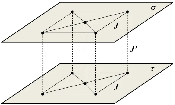
FIG. 1. Visualisation of the model as two planes σ and τ. The long-ranged intraplane interaction isJ and the short-ranged interplane interaction isJ′.
The above description suggests that constituents of each component interact with one an-other via long-range (mean-field) interactions Ja and with spins from the other compo-nent locally via the short-ranged (local) interactions J′
ab. For simplicity, we assume that Jσ =Jτ =J, Jστ′ =Jτ σ′ =J′ and that the number of spins in both components is the same Nσ =Nτ =N.
A helpful way of visualising this system is depicted in Fig. 1 where we consider theσandτ components lying on two different parallel planes. We will use this graphic interpretation as it conveniently separates the global and local interactions and simplifies the nomenclature we will be using. The long-range interaction defined by the couplingJ will be termed intraplane interaction, while J′ will define the local and symmetric interplane interaction.
The system is updated synchronously, meaning that at each time step all the spins are updated simultaneously; the generating functional method [20] then allows for the dynamics to be solved exactly. This results in a two-dimensional non-linear dynamical map for the magnetisations of the different components of the system given by
mσ(t+ 1) =htanhβσhσ(t)iτ(t), (5)
where
hσ(t) =Jmσ(t) +J′τ(t), (7)
hτ(t) =Jmτ(t) +J′σ(t), (8)
and where averages h•iare with respect to the corresponding probability distributions
P[σ(t)] = 1
2[1 +σ(t)m
σ(t)], (9)
P[τ(t)] = 1
2[1 +τ(t)m τ
(t)]. (10)
The steady state solutions are given by the fixed points of this map
mσ =
htanhβσ(Jmσ+J′τ)
iτ, (11)
mτ =
htanhβτ(Jmτ +J′σ)iσ, (12)
which are exactly the same equations that describe, in equilibrium, the magnetisation of a spins system with long-range interactions subjected to a random magnetic field. These fixed points are analysed in the following section.
III. STEADY STATES
Steady state solutions of the dynamics of our system will be given by the fixed points of the two-dimensional map defined by equations (5) and (6). A notational simplification of those equations can be achieved by using the reduced variables ˜βa = J′βa and ˜J = J/J′, resulting in the following map
f(mσ, mτ) = (fσ, fτ),
fσ = 1 2
X s
(1 +smτ) tanh ˜β σ
˜
Jmσ +s, (13)
fτ = 1 2
X s
(1 +smσ) tanh ˜β τ
˜
Jmτ +s,
It is possible to obtain the fixed points of these equations numerically for any parameter set. Still, it is interesting to study the behaviour of the system in the limits of high and low temperatures, which can be obtained analytically and exposes a very rich phase diagram. The latter represents different types of interactions between the systems components and provides insights into the corresponding macroscopic properties.
The system, as defined, is symmetric under exchange of component labelsσ ↔τ. There-fore, without loss of generality, we choose the τ-component to be connected to a thermal reservoir at high temperature ˜βτ →0. Then
fτ ≈β˜τ
˜
Jmτ +mσ, (14)
resulting in the fixed point
mτ = ˜β
τmσ, (15)
at leading order in ˜βτ.
Naturally, at high temperature the intraplane interaction ˜J is not sufficiently strong to influence the spins alignment and disappears from the equation. The interplane interaction still survives, although weakened by the thermal disorder, linking the magnetisations of the two components via a proportionality constant ˜βτ; the relative sign between the two is determined by the nature of the interaction J′ (ferromagnetic or antiferromagnetic) in an obvious way.
When the τ-component temperature becomes infinite, with ˜βτ being exactly zero, the intraplane interaction becomes too weak to allow for the interaction with the σ-component to affect the τ-component alignment, which then leads to a paramagnetic phase with mag-netisation mτ = 0. It is easy to see that consequently the σ-component becomes equivalent to a mean-field Ising model in a random field of zero mean [22].
Keeping the τ-component’s temperature fixed at a high but finite value, one can re-examine the system’s properties at various temperature limits of the σ-component. For the case of high temperature (low ˜βσ), one obtains a proportionality relation between the magnetisations
mσ = ˜β
σmτ ⇒mτ = ˜βτβ˜σmτ. (16)
-1.5 -1.0 -0.5 0.0 0.5 1.0 1.5 -1.5
-1.0 -0.5
0.0 0.5 1.0 1.5
mΣ
fΣ
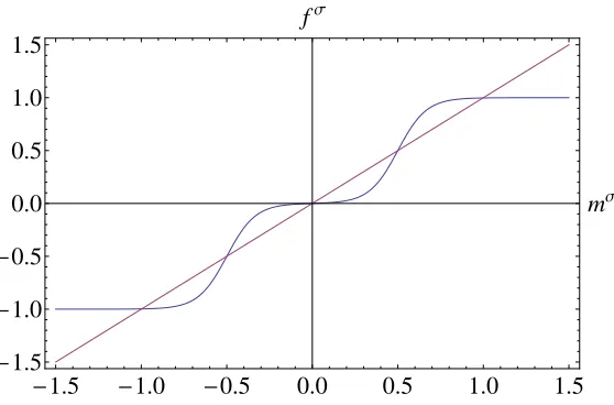
FIG. 2. Fixed points of the magnetisation mσ forJ = 2 and ˜β σ = 3
to what we conventionally refer to as the global paramagnetic (GP) phase. The GP phase is a ubiquitous fixed point, present for any temperature, but its uniqueness and stability are temperature-dependent. In this section we will focus on its uniqueness property, i.e., analyse the existence of other possible phases in these temperature limits. The issue of its stability will be addressed mainly in the next section.
One notable feature of the high-temperature regime inτ is that it is rich enough to develop a total of either three or five fixed points as the σ-component’s temperature decreases, depending on the values of the intraplane interaction J′. This can be obtained from the relation between fσ and mσ of Eq. (13) by utilising the high temperature relation (15)and the intersection of fσ with the line mσ. Figure 2 shows an exemplar plot for ˜J = 2 and
˜
βσ = 3. The graph shows five fixed points: a stable solution atmσ = 0, two stable solutions at high magnetisation values (largest) and two unstable solutions at intermediate values.
For τ at high temperature and at the limit |β˜σ| → ∞ one obtains
mσ =Dsgn ˜βσ
˜
Jmσ +τE
τ = sgnJ ′
·DsgnJm˜ σ+τE
τ. (17)
In this case, one has to consider the various possible values for the intraplane interaction ˜
J. For |J˜|<1
mσ =mτsgn ˜βσ =mτsgnJ′, (18)
σ-system. A straightforward, but lengthy consideration of the possibilities for |J˜|= 1 gives the same result. This means that there are situations where the GP phase is the only phase present at the high-temperature βτ → 0 limit for both low and high Tσ; which reveals the importance of the relative (non-dimenionalised) interaction strength ˜J in defining the state of the combined system, rather than their actual individual values.
Non-GP solutions do exist for |J˜|>1. When|Jm˜ σ
|>1 we have
mσ = sgnJ·sgnmσ, (19)
and mσ becomes independent of mτ. Ignoring the GP solution, we are left with mσ = ±sgnmσ depending on the sign of the intraplane interaction.
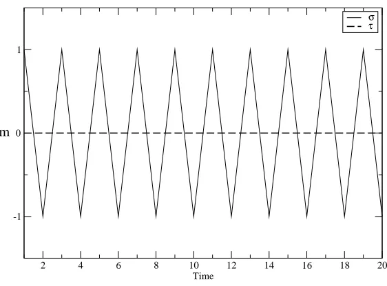
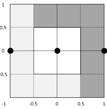
It is convenient to consider several different cases: (i) A positive sign gives mσ = ±1, meaning that the intraplane interaction is sufficient to align the σ component spins com-pletely, independently of the heat flow from the τ to the σ-components. (ii) A negative sign results in oscillations between ±1, a cycle of period 2 for mσ instead of a fixed point as depicted in Fig 3. This occurs, for instance, in the case antiferromagnetic intraplane interactions and is characteristic of synchronous update dynamics. (iii) Finally, the case
˜ Jmσ =
±1 has as the non-GP solutions
mσ =± sgnJ ′
2−β˜τ
, (20)
which exist when the interactions obey the temperature-dependent condition ˜J = (2 − ˜
βτ) sgnJ′. This means that for each ˜βτ value only one solution exists on the ˜J line.
As the equations are completely symmetric with respect to exchanges of σ and τ, the only remaining case is the one where both systems are at low temperatures with Tτ, Tσ ≪ 1, or equivalently |β˜τ|,|β˜σ| ≫ 1. Once more we consider separately cases with different magnitudes of the interactions:
(a) For|J˜| <1 we have
fσ =mτsgnJ′, (21)
fτ =mσsgnJ′. (22)
2 4 6 8 10 12 14 16 18 20 Time
-1 0 1
m
σ τ
FIG. 3. Dynamics of the 2D map of the magnetisations for βτ = 10−2, βσ = 102, J = −5 and
J′= 10−2. The period 2 cycle inm
σ sets in already at the first iteration, whilemτ remains at zero mainly due to its very high temperature.
(b) When |J˜|= 1, the same solution is obtained for |mσ|,|mτ| < 1, but when |mσ| = |mτ|= 1 the fixed points mσ =mτsgnJ′ occur only for sgnJ′ = ˜J; otherwise the solutions are period-2 cycles.
(c) The |J˜|>1 case is more complicated to analyse. Here the intraplane interaction is relatively strong and many different solutions can be found. We have to take into consider-ation one of the three cases for each of the magnetisconsider-ations (a, b=σ, τ):
|Jm˜ a
|>1⇒fa = sgnJ
·sgnma,
|Jm˜ a|= 1 ⇒fa = m b
2sgnJ′−J˜, |Jm˜ a|<1⇒fa =mbsgnJ′.
(23)
(i) The case of |Jm˜ σ| > 1 and |Jm˜ τ| > 1 results in two independent equations of the form (19) for each one of the magnetisations, giving completely aligned states or period-2 cycles for all points with |mσ| > 1/|J˜| and |mτ| >1/|J˜|. (ii) Another simple case is when |Jm˜ σ
|<1 and |Jm˜ τ
|<1, or equivalently |mσ
|<1/|J˜| and |mτ
|<1/|J˜|, which reduces to the same set of solutions as for|J˜|<1.
(iii) When |Jm˜ σ|=|Jm˜ τ|= 1, or|mσ|=|mτ|= 1/|J˜|, the equations become
mσ = m
τ
2sgnJ′−J˜, m
τ = m σ
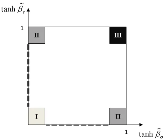
FIG. 4. Partial phase diagram for the limiting cases of high and low temperatures. The figure shows only the first quadrant as the other three are simply its symmetrical images reflected about the axes. On the dashed axis, the corresponding magnetisation is zero as the temperature is infinite.
which exists when the interactions obey the relation 2sgnJ′ −J˜= ±1. For the plus sign, we have fixed points where mσ =mτ, while the minus sign gives mσ =−mτ.
It remains to analyse the mixed cases with: (iv) |Jm˜ a| > 1, |Jm˜ b| < 1; (v) |Jm˜ a| > 1, |Jm˜ b|= 1; (vi) |Jm˜ a|<1, |Jm˜ b|= 1.
Cases (iv) and (v) can only have non-GP phases for ma =
±1 and sgnJ = +1 and a 2-period oscillatory behaviour when sgnJ = −1 with ma oscillating between +1 and −1. In both cases, mb will be a multiple of ma according to the corresponding value given by one of the equations (23). Finally, all points in case (vi) are either fixed points, when 2−J˜sgnJ′ = +1, or 2-period cycles, when 2−J˜sgnJ′ =−1
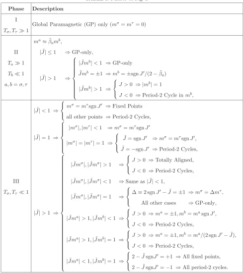
Figure 4, together with table I, presents a summary of the possible asymptotic phases of the system in the limits we analysed. Intermediate regimes are more difficult to analyse, but the equations are simple enough to be solved numerically for any parameter values.
TABLE I. Phases of Fig 4. Phase Description
I
Tσ, Tτ ≫1
Global Paramagnetic (GP) only (mσ =mτ = 0)
II
Ta≫1
Tb ≪1
a, b=σ, τ
ma≈β˜ amb,
|J˜| ≤1 ⇒GP-only,
|J˜|>1 ⇒
|Jm˜ b|<1 ⇒GP-only ˜
Jmb =±1 ⇒mb =±sgnJ′/(2−β˜ a)
|Jm˜ b|>1 ⇒
J >0 ⇒ |mb|= 1
J <0 ⇒Period-2 Cycle in mb,
III
Tσ, Tτ ≪1
|J˜|<1 ⇒
mσ =mτsgnJ′ ⇒Fixed Points all other points ⇒Period-2 Cycles,
|J˜|= 1 ⇒
|mσ|,|mτ|<1 ⇒mσ =mτsgnJ′
|mσ|=|mτ|= 1 ⇒
˜
J = sgnJ′ ⇒mσ =mτsgnJ′, ˜
J =−sgnJ′ ⇒Period-2 Cycles,
|J˜|>1 ⇒
|Jm˜ σ|,|J m˜ σ|>1 ⇒
J >0 ⇒Totally Aligned, J <0 ⇒Period-2 Cycles,
|Jm˜ σ|,|J m˜ σ|<1 ⇒Same as |J˜|<1,
|Jm˜ σ|,|J m˜ σ|= 1 ⇒
∆≡2 sgnJ′−J˜=±1 ⇒mσ = ∆mτ, All other cases ⇒GP-only,
|Jm˜ a|>1,|J m˜ b|<1 ⇒
J >0 ⇒ma=±1, mb =masgnJ′,
J <0 ⇒Period-2 Cycles,
|Jm˜ a|>1,|J m˜ b|= 1 ⇒
J >0 ⇒ma=±1, mb =ma/(2 sgnJ′−J˜),
J <0 ⇒Period-2 Cycles,
|Jm˜ a|<1,|J m˜ b|= 1 ⇒
2−J˜sgnJ′ = +1 ⇒All fixed points, 2−J˜sgnJ′ =−1 ⇒All period-2 cycles.
IV. STABILITY OF THE GP PHASE
As previously noted, there are two different types of paramagnetic phases in the presented model: (i) the GP phase wheremσ =mτ = 0, and the (ii)a-component paramagnetic phases, where ma = 0, with a either σ or τ and the magnetisation of the other component being non-zero.
The GP phase is ubiquitous in the studied model, being always a solution for any combi-nation of parameters. However, depending on the values of these parameters, the stability of this phase can drastically vary; it can be analysed by calculating the eigenvalues of the Jacobian matrix of our two-dimensional map. This general form of the matrix is
Df =
∂fσ/∂mσ ∂fσ/∂mτ
∂fτ/∂mσ ∂fτ/∂mτ
=
βσJ D
sech2β˜σ
˜
Jmσ +τE τ
1 2
P
s=±1tanh ˜βσ( ˜Jmσs+ 1) 1
2
P
s=±1tanh ˜βτ( ˜Jmτs+ 1) βτJ D
sech2β˜τ
˜
J mτ +σE σ
.
(25)
For the GP phase, atmσ =mτ = 0, the Jacobian matrix simplifies to
Df =
βσJsech2β˜σ tanh ˜βσ tanh ˜βτ βτJsech2β˜τ
, (26)
with eigenvalues
λ±= 1 2(−b±
√
∆), (27)
where
b=−Jβσsech2β˜σ+βτsech2β˜τ
, (28)
∆ = J2βσsech2β˜σ−βτsech2β˜τ 2
+ 4 tanh ˜βσtanh ˜βτ. (29)
For ˜βτ = ˜βσ = 0, both eigenvalues are zero indicating that the GP phase is a sink, i.e., stable to perturbations. For small, but non-zero inverse temperatures (high-temperature limit), we have
λ±
≈ 12[J(βσ +βτ)± |J(βσ−βτ)|], (30)
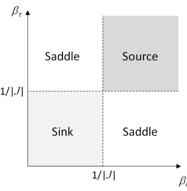
FIG. 5. Stability of the GP phase for high temperatures (small β’s).
becomes unstable below some temperature value. For either βσ &1/|J| orβτ &1/|J| sepa-rately, it becomes a saddle. If both conditions are satisfied it becomes a source. Note that these conditions are exactly the ones defining the critical point of the naive mean field Ising model. The results for high temperatures are indicated in Fig 5.
The results for low temperatures with βσ, βτ → ∞are
λ±≈ ±1 + 2J(βσe−2 ˜βσ +βτe−2 ˜βτ), (31)
and the GP is always a saddle.
An interesting case occurs in the regime where one of the temperatures is high and the other is low. By taking βτ →0 and βσ → ∞, straightforward calculations show that
λ±≈J 2βσe−2βσ +βτ
±p|J′|β
τ. (32)
For sufficiently large values this points to a stability of the GP phase for all interaction values. This can be seen from the basin of attraction depicted in Fig. 6. The figure shows the basin of attraction for fixed points of the two-dimensional map (13) with parameters given by J = 2, J′ = 1, β
FIG. 6. Basin of attraction for values J = 2,J′ = 1,β
σ = 103 and βτ = 0.
V. CONCLUSIONS
With the aim of understanding the behaviour of non-equilibrium systems with two-temperatures, we introduced and solved a simple model of a system comprising two spin-1/2 components, referred to as the σ and τ components; these are coupled to separate thermal reservoirs held at different temperaturesTσ andTτ, respectively. For visualisation purposes, we considered the two system components as belonging to two different planes. Each com-ponent has then an intraplane long-ranged mean-field interaction J while it interacts with the other component via an interplane local interaction J′.
Using the generating functional technique we have found a pair of exact, self-consistent coupled equations for the magnetisations of the two components mσ and mτ, the solution of which is given by the fixed-points of the resulting two-dimensional non-linear map. This map depends on three degrees of freedom which are given by the ratio between the inter and intra-component couplings ˜J =J/J′ and the scaled inverse temperatures of each component
˜
βσ =J′βσ and ˜βτ =J′βτ.
The analysis of the particular phase where both components have zero magnetisation, which we termed the Global Paramagnetic (GP) phase, show that the stability of this phase has some interesting characteristics, especially in the low and high temperature limits. We have not found any evidence for chaotic behaviour in general, but have no definitive proof either for its existence or absence as each orbit would need to be analysed individually. We conjecture that this is due to the nature of the stochastic dynamics that give rise to this mapping as the magnetisations fluctuate very close to the mean values at the large system limit which we investigate.
The framework introduced and the results obtained can be easily modified to accommo-date other cases; one obvious modification being the spatial nature (local/non-local) of the interactions. Also, with the appropriate changes, one can apply this theory to several other non-equilibrium practical situations where a steady state is reached.
One of these cases, which we are currently exploring, is related to astrophysical dark matter as the dark sector might have, in additional to its gravitational coupling to the visible sector, exclusive dark matter interactions. This opens up the possibility of systems at different temperatures to co-exist at the same physical location but in different sectors. These systems can then be heated independently by processes on their own sectors and exchange energy only via gravitational interactions. The current framework could be modified to accommodate long-range gravitational “interplane” interaction and short-rang “intraplane” interaction according to bounds obtained from astrophysical observations [21]. Analysis of the phases and the heat-transfer between both sectors could shed light on the nature of these potential interactions or serve as an additional detecting mechanism.
Another extension of this framework, which is also under way, is the application to superlattices [23]. Superlattices are metamaterials constructed of alternate layers of two different materials that hold useful properties. In a forthcoming study, we appropriately alternate thermal conducting magnetic layers with thermal isolating ones such that each one of n >2 conducting layers can be coupled to a different thermal reservoir. This would result in an n-temperatures systems and the magnetisations would then be described by an n-dimensional non-linear map with the promise of a rich and interesting phase diagram.
particularly simple case of interacting magnetic systems held at different temperatures, can be carried out rigorously and paves the way to better understanding of similar cases in a variety of fields.
ACKNOWLEDGMENTS
Support by the Leverhulme trust (F/00 250/M) is acknowledged. A.C. would like to acknowledge Dr Banibrata Mukhopadhyay of the Indian Institute of Science, Bangalore, for useful discussions.
[1] S. Lepri, R. Livi and A. Politi, Phys. Rep. 377, 1 (2003). [2] A. Dhar, Adv. Phys. 57, 457 (2008).
[3] A. Dhar and J. L. Lebowitz, Phys. Rev. Lett. 100, 134301 (2008).
[4] A. Dhar, K. Venkateshan and J. L. Lebowitz, Phys. Rev. E83, 021108 (2011).
[5] A. Kundu, S. Sabhapandit and A. Dhar, J. Stat. Mech.: Theory and Expt., P03007 (2011). [6] T. Yamada and K. Kawasaki, Prog. Theo. Phys.38, 1031 (1967).
[7] G. N. Bochkov and Yu. E. Kuzolev, Physica 106A, 443 (1981). [8] C. Jarzynski, Phys. Rev. Lett. 78, 2690 (1997).
[9] A. K. Chattopadhyay, Phys. Rev. E 84, 032101 (2011). [10] K. Saito and A. Dhar, Phys. Rev. Lett.107, 250601 (2011). [11] T. Bodineau and B. Derrida, Phys. Rev. Lett. 92, 180601 (2004). [12] A. Dhar, D. Sen and D. Roy, Phys. Rev. Lett. 101, 066805 (2008). [13] V. S. Dotsenko, Phys. Usp. 36, 455 (1993).
[14] V. Dotsenko, An Introduction of the Theory of Spin Glasses and Neural Networks, World Scientific (1994).
[15] J. van Mourik and A. C. C. Coolen, J. Phys. A 34, L111 (2001). [16] D. N. Spergel and P. J. Steinhardt, Phys. Rev. Lett.84, 3760 (2000). [17] J. L. Feng, H. Tu and H. -B. Yu, JCAP10, 043 (2008).
[19] I. K. Schuller, Phys. Rev. Lett.44, 1597 (1980). [20] D. Saad and A. Mozeika, Phys Rev E, in press.
[21] B. A. Gradwohl and J. A. Frieman, Astro. J. 398, 407 (1992).
[22] H. Nishimori,Statistical Physics of Spin Glasses and Information Processing, Oxford Univer-sity Press (2001).