ORIGINAL PAPER
Spectral density estimation of European airlines load factors
for Europe-Middle East and Europe-Far East flights
Yohannes Yebabe Tesfay&Per Bjarte Solibakke
Received: 18 July 2014 / Accepted: 3 March 2015 / Published online: 16 April 2015 #The Author(s) 2015. This article is published with open access at SpringerLink.com
Abstract
PurposeIn the airline industry the term load factor is defined as the percentage of seats filled by revenue passengers. The load factor is a metric that measures the airline’s capacity and demand management. This paper aimed to identify serial and periodic autocorrelation on the load factors of the Europe-Mid East and Europe-Far East airline flights. Identifying the auto-correlation structure is helpful to develop the best fitted fore-casting model of the load factors.
Methods The paper applies spectral density estimation to investigate the structure of serial and periodic autocor-relation on the load factors. Then the paper applied multivariate trend model to develop a forecasting model of the load factors of the regional flights. The
multivar-iate trend model is fitted using the Prais–Winsten
recur-sive autoregression methodology.
ResultsThe primary analysis of the study identified that the airlines have better a demand than capacity management sys-tem for both the Europe-Mid East and Europe-Far East flights. The spectral density estimates showed that the load factors have both periodic and serial correlations for both regional flights. Therefore, in order to control the periodic autocorrela-tion, we introduce transcendental time functions as predictors of the load factor in the multivariate trend model. Finally, we build realistic and robust forecasting model of the load factors of the Europe-Mid East and Europe-Far East flights.
Conclusions The econometric estimation results confirm that the load factors of the Europe-Mid East and Europe-Far East
flights are both seasonal and differ between flights. The anal-ysis implies that the load factor is still far from stable and stabilizing policies by airlines has so far not been successful. The AEA may therefore continuously focus on the stabiliza-tion and the improvement of the load in the industry.
Keywords Airlines . Load factor . Spectral density estimation . Multivariate trend analysis
1 Introduction
The yield, revenue per unit of output sold, is a highly signif-icant metric in the airline industry. By definition, it is only the mathematical outcome of two even more fundamental met-rics: output sold and revenue earned. For more than five de-cades the yields across the industry as a whole has been in decline. These price declines explain a significant portion of
the traffic growth throughout the period [33]. Broadly
speak-ing, the yields will soften when (1) traffic growth is flat or insufficient to absorb output growth, (2) intense competition lower prices, and yields will harden when (2a) load factors are already high and output is growing slower than traffic, (2b) traffic growth is outstripping growth in output and (3) lower competition keeps prices unchanged. The fact that traffic, load factor, and revenue all will be affected by these type of adjust-ments, illustrates how intimately connected the variables are—all within the context of available output [37,38].
This paper’s main variable of interest is the airline industry load factor. The load factor measures the percentage of an
airline’s output that has been sold to paying passengers.
Hence, the load factor is a measure of the extent to which supply and demand are balanced at prevailing prices. The achieved load factors for the industry as a whole conceal marked variations between different type of airliners, with regional carriers at the lower end of the spectrum and charter
This article is part of the Topical Collection on Accessibility and Policy Making
Y. Y. Tesfay (*)
:
P. B. SolibakkeMolde University College, Britveien 2, Kvam, 6402 Molde, Norway e-mail: yohannesyebebabe@gmail.com
P. B. Solibakke
airlines generally achieving higher load factors than
sched-uled carriers [8]. The average load factors for individual
airline enterprises masks variations between different mar-kets and cabins. Economy cabins achieving higher load factors because customers tend to book further in advance and expect lower levels of seat accessibility than for pre-mium cabins. The average load factors in the airline indus-try also conceal pronounced daily, weekly and, in particu-lar, seasonal variations.
There are at least six load factors drivers in the airline
industry. Thefirstdriver is the industry’s output decisions
relative to demand growth. The output growth must be
brought into alignment with demand growth. Thesecond
driv-er is pricing. Fare reductions gendriv-erally stimulate demand. Load factors are affected depending upon capacity decisions. Thethirddriver is the traffic mix. Historically, the higher the proportion of business travellers carried by an airline, the low-er the avlow-erage seat factor. That is, the random element in demand for business travels (highly volatile demand) suggests a lower average load factor in business and first class cabins [31]. Thefourthdriver is refund policies. A carrier taking non-refundable payment at the time of reservation is likely to have relatively few no-shows and a relatively higher seat factor than carriers selling a high portion of fully flexible tickets. Thefifth
driver is commercial success. A success of product design, promotions, marketing communications, distributions, and
service delivery will influence load factors. Thesixthdriver
is revenue management. The effectiveness of revenue man-agement systems (RMS) will influence load factors. The RMS capabilities, specifically the refinement of demand forecasting
tools, will contribute significantly [30]. Depending on market
conditions in the airline industry, there exist a trade-off be-tween load and yield. Unless demand is particularly strong and output growth is under firm control, it is likely that rising yields will be associated with downward pressure on load factors. In contrast, a falling yield tends to be associated with higher load factors. The trade-off suggests that airline carriers will generally want to arrive at a capacity, which targets a load factor balances between the costs of turning passengers away and the costs of meeting all peak demand and oversupplying
the market (Bdouble-edged sword^). In general, therefore,
from an operational perspective it is easier to manage an air-line when load factors are at 64 % than when they are at 84 % [9]. The size of the load factor is therefore a measure of suc-cess in the airline industry. However, the sucsuc-cess factor is challenged by the fact that demand is volatile and fluctuates in units of single seat-departures in different origin and desti-nation markets. In contrast, the capacity can only be delivered in units of available aircrafts for the particular flight-leg. That is, routes designed to serve the origin and destination markets are broadly fixed in the short run. Furthermore, the necessity to maintain both high flight completion rates, the integrity of network connections, and aircraft/crew assignments, may
make it almost impossible for a scheduled passenger carrier to cancel a significant number of its lightly loaded flights [4]. The main objective of this paper is to build econometric models that can capture the variations of load factors for Europe-Middle East and Europe-Far East airline flights. The
paper’s target population is airlines that are members of the
Association of European Airlines (AEA). We use multivariate time series econometric model to analyse the temporal evalu-ation of load factor. The best well-fitted econometric model may improve the accuracy of forecasting the load factor of these specific flights. However, in order to build the best fitted model for the load factor we are encountered to several chal-lenges. First, we need to evaluate characteristics of available seat kilometre and revenue passenger kilometre on the load factor. Second, we need to have solid knowledge about the autocorrelation structure of the load factor. Classically, we think that the intensity of autocorrelation of time series data diminishes with more distant lags.
However, in reality, the true autocorrelation structure of the load factor has the periodic autocorrelation (i.e., load factor it is highly seasonal). Consequently, we have to identify the structure of both serial and periodic autocorrelations on the load factor. Third, once we identify the autocorrelation struc-ture of the load factor, then we will deal with mechanisms to control it during model fit.
In this study, we advance the classical multivariate trend analyses to control the periodic autocorrelation by expressing the time effect of the load factor as a dynamic (can be linear or
nonlinear) function of the parameters [29]. Furthermore, in
order to control for the serial autocorrelation we apply Prais–
Winsten recursive autoregression estimation [34]. Finding the
best suitable mathematical relationships of the dynamic time effect of the load factor and controlling serial correlation is therefore the most important task of this study. The best fitted econometric model may bring superior forecasting tools and techniques, and new information to the AEA.
2 Literature review
The airline industry plays an essential role in the establishment
of today’s global economy. According to Doganis [15] the
airline industry gives the impression of being both cyclical and strappingly subjective to external dynamics. The interna-tional airline industry is complex, dynamic, subject to rapid change, innovation, and marginally profitable. By considering
procedures determining tariff levels in an origin‐destination
market, airline pricing refers to various service facilities and capacities for a set of airline products.
the success of the airline is determined by its ability to make unit revenues (i.e., the product of yield and load factor) higher than its unit costs. Therefore, in addition to minimize the unit cost, the important task of the airline manager is to simultaneously maximize the product of
yield and load factor [21].
Yield management is the assortment of schemes, strat-egies and tactics the airline enterprises use to
systemati-cally manage demand for their services and products [25].
The fundamental units for yield management are load
fac-tors, pricing and cost of the airlines [26]. Passenger load
factor (or only load factor) is a measure of the degree of airline passenger carrying capacity. The load factor is a quantity of the extent to which supply and demand are
balanced at prevailing prices [18]. In short, load factor is
defined as the ratio of the revenue passenger kilometre to available seat kilometre in the given origin destination flight [14,4].
The load factor is a measure of the performance and effi-ciency of an airline. The airline’s load factor directly reflects their competency and performance. The high load factor with appropriate pricing is a condition for the efficient operation of an airline enterprise [40]. Thus, it is enlightening for the per-formance of the airline to highlight factors that affect the load factors [22].
Generally, operational factors play a significant role in affecting the load factor and therefore capacity. Specifi-cally, operational factors such as distance covered by jour-ney, tourists, codeshare agreement (is an aviation business arrangement where two or more airlines share the same flight) and market concentration HHI index (a commonly accepted measure of market concentration) are among the most important factors that have positive and significant
effect on the load factor [32]. Moreover, the GINI index
(a measure the degree of price dispersion, or price in-equality in the airline of the same flight) is discovered as the main factor that negatively affects the load factor. Other important factors are airport features, performance limitation, flight conditions, seasonality of demand, time of traveller schedule, frequency of flights and dynamic
route networks [32,24].
3 The data and methodology
3.1 The data
The dataset is obtained from theAssociation of European
Airlines (AEA)and is downloaded fromhttp://www.aea.be/ research/traffic/index.html. The data is collected for the period 1991 to 2013 and contains information about
Available Seat-Kilometres (ASK), Revenue
Passenger-Kilometres (RPK) and Load factor (LF).
Moreover, Europe-Far East (EF) is defined as any
scheduled flights between Europe and points east of the Middle East region, including Trans-Polar and
Trans-Siberian flights. Europe-Middle East (EM) is
de-fined as any scheduled Terminating flights between Eu-rope and Bahrain, Iran, Iraq, Israel, Jordan, Kuwait, Lebanon, Oman, Saudi Arabia, Syria, United Arab Emirates, Yemen and the Democratic Republic of
Ye-men (Available at www.aea.be).
3.2 Methodology
3.2.1 One way analysis of variance (ANOVA)
One way analysis of variance (ANOVA) is used to see the existences of the main differences of a certain random variables with a single treatment over its levels. The linear statistical model for ANOVA is giv-en as([6, 43]:
yi j¼μþαiþεi j; i¼1;2;3;…;a and j
¼1;2;3;…;n ð1Þ
where: μ the grand mean of yij, αi the ith level effect
on yij and εij∼iidN(0,σ 2
). The bootstrapping estimation method is applied to estimate the model parameters. Usually the method of estimation of the model param-eters is either using ordinal least square (OLS) or gen-eralized least square (GLS) estimators according to the
parameters are fixed or random, respectively [17, 11].
Nevertheless, modern econometric methods used bootstrapping to acquire thorough information about the estimated parameters. In this particular case we apply the Bias-Estimation Bootstrap technique. The es-timation method gives information about bias of the estimates due to resampling in addition to the estimates
of OLS or GLS [13].
3.2.2 Signal processing
Signal processing represents a time series as a stochastic sum
of harmonic functions of time [20]. Signal processing helps to
identify the autocorrelation structure of the time series data. The signal processing stochastic model for stochastic process in discrete time is given as [23,35]:
yt¼μ*t þX k
akcos 2ð πυktÞ þbksinð2πυktÞ
½ ð2Þ
Where:μt∗is the mean of the series at timet,ak,bk(Fourier
independent zero mean normal random variables,vkare
dis-tinct frequencies.
The mean, variance and covariance of the spectrum of the time series data are derived as follows:
E y½ ¼t E μ*t þE X k
akcos 2ð πυktÞ þbksinð2πυktÞ
½
( )
E y½ ¼t μ*t þ X k
E a½ kcos 2ð πυktÞ þbksinð2πυktÞ
∴E y½ ¼t μ*t
ð3Þ
V a r y½ ¼t E f½ −yt E y½ tg2
V ar y½ ¼t E μ*tþ
X
k
akcos 2ð πυktÞ þbksinð2πυktÞ
½ −μ*
t
( )2
∴V a r y½ ¼t E X k
akcos 2ð πυktÞ þbksinð2πυktÞ
½
( )2
ð4Þ
Cov y½ t;yt−τ ¼Efðyt−E y½ tÞðyt−τ−E y½ t−τÞg ð5Þ
S i n c e yt−E y½ ¼t ∑ k
akcosð2πvktÞ þbksinð2πvktÞ
½ a n d
yt−τ−E y½ t−τ ¼∑ k
akcosð2πvkt−τÞ þbksinð2πvkt−τÞ
½
Therefore, Eq.5can be expressed as:
Cov y½ t;yt−τ ¼E
f
Xk
akcos 2ð πvktÞ þbksin 2ð πvktÞ
½
!
X
k
akcos 2ð πvkt−τÞ þbksin 2ð πvkt−τÞ
½
!
g
g
ð6Þ
Spectral density is a powerful tool to analyse the nature of the autocorrelation of the time series data in the Fourier space that contains infinite sum of sine and cosine waves of different
amplitudes [16,3]. This creates good prospect to remove the
problem of autocorrelation and to choose appropriate an econometric model that capture the possible variations of the time series data. Estimation techniques of spectral density can involve parametric or non-parametric approaches based on time domain or frequency domain analysis. A common para-metric technique involves fitting the observations to an autoregressive model. A common non-parametric technique
Table 1 Estimates of RPK (in million) and ASK (in million) of the EM and EF flights
Flights Estimates of Revenue Passenger Kilometre (RPK in million) Estimates of Available Seat Kilometre (ASK in million)
Statistic Estimates Bias Std. Error
95 % Confidence Interval
Statistic Estimates Bias Std. Error
95 % Confidence Interval
Lower Upper Lower Upper
EM-Flights Mean 1696.92 1.863 42.52 1617.65 1784.05 Mean 2450.76 1.53 56.82 2333.1 2566.78 Std. Deviation 729.94 −2.44 24.39 680.11 774.73 Std. Deviation 936.96 −3.0 30.01 869.19 991.55
Std. Error Mean 43.94 Std. Error Mean 56.40
EF-Flights Mean 9671.81 −1.77 185.7 9317.00 10,023.0 Mean 12,375.32 10.46 193.21 12,005.0 12,754.61 Std. Deviation 3059.35 −6.34 95.64 2853.89 3229.34 Std. Deviation 3292.10 −5.48 99.73 3089.31 3486.857 Std. Error Mean 184.15 Std. Error Mean 198.16
Estimation Method
Bootstrap results are based on 1000 bootstrap samples
Table 2 Comparison of ASK, RPK and load factor of EM and EF flights
Variables Comparison of flights Mean Difference Std. Error Difference t-cal Sig. (2-tailed) 95 % Confidence Interval of mean difference
Lower Upper
is the periodogram. The important advantage of applying the periodogram spectral estimator is determining possible hidden Bperiodicities^in the time series [36].
3.2.3 Ljung–Box test
There are a number of parametric methods that detect
auto-correlation. However, the Ljung–Box test is preferable in this
case because it simultaneously detects the existence and the
order of autocorrelation on the time series data. The Ljung–
Box test procedure is given as [10]: the Null HypothesisH0:
serial correlation equals zero up to order h versusH1: at least
one of the serial correlations up to lag h is nonzero. The test statistic of Ljung–Box is given as:
Q¼n nð þ2ÞX h
l−1
b ρ2
l
n−l ð7Þ
where:nis the sample size,bρlis the sample autocorrelation at
lagl, andhis the number of lags being tested. The null
hy-pothesis is rejected forαlevel of significance ifQ>χl2−α,h.
3.2.4 Multivariate trend analysis
The aim of the trend analysis is to get the best fitted model to be applied for forecasting the long run behaviour of the series
as a function of time [28]. The general form of multivariate
trend analysis is given as [5,41].
yit¼ fiðt;βiÞ þεit ð8Þ
εit ¼U εit−1;εit−2;…εit−h;ρi1;ρi2;…;ρihi
þvit a n d vi t~ iiDN(0,σiv2) where:fi(t;βi) is any real valued function of time
Bt^and a vector of parametersβi¼ βi0;βi1;βi2;…;βiki
,U
εit−1;εit−2;…εit−h;ρi1;ρi2;…;ρihi
is a linear function ofεit−
ij,ρijandj=1,2,3,….hi,εitandvitare random error terms.
To find suitable estimation method of the model param-eters, it is necessary to have acquaintance about the math-ematical structure offi(t;βi). In this case we have two major
categories of fi(t;βi), linear and nonlinear models [41]. If
the model is linear then we simply apply the ordinary least square (OLS) estimation method to estimate the model pa-rameters [39,20].
3.2.5 Steps of controlling serial autocorrelation
After controlling for periodic autocorrelation by setting the time effects as a function of time, we need to remove the serial correlation. Therefore, the following steps (algorithm) are used to remove serial correlation:
Step 1: First estimate the model fit residuals as [43,7]:
b
εit ¼yit−fi t;βbi
ð9Þ
Step 2: Determine the structure of autocorrelation. At this
step we use the Ljung–Box test of autocorrelation.
Step 3: If we do not reject our null-hypothesis we take the model fit is free from the problem of autocorrelation.
Otherwise, we apply the Prais–Winsten estimation
recursive estimation to remove serial correlation [44,19,42,12,1,34]. The estimated variance co-variance matrix is given as:
Table 3 Prais-Winsten recursive parameter estimation of a linear
regression of RPK (in million) in response to ASK (in million)
Predictor Estimators Std. Error
t-cal Sig. R Square Model Std. Error
ASK 0.776 0.013 58.912 0.0000
Constant −205.356 34.683 −5.921 0.0000 0.927 115.788
Key: ASK RPK
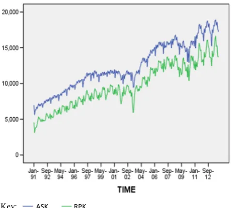
Fig. 1 Time Series Plot of ASK and RPK (in million) of EM flights
Table 4 Prais-Winsten recursive parameter estimation of a linear
regression of RPK (in million) in response to ASK (in million)
Predictor Estimators Std. Erro
t-cal Sig. R Square Model Std. Error
ASK 0.914 0.015 59.147 0.0000
b Ωi¼
1 1−bρ2i
1 bρi bρ2i ⋯ bρni−1 b
ρi 1 bρi ⋯ bρ n−2
i b
ρ2 bρ ⋱ ⋯ ⋮
⋮ ⋮ 1 bρi bρn−1
i bρ n−2
i ⋯ bρi 1
2 6 6 6 6 4
3 7 7 7 7
5 ð10Þ
The inverse of the variance covariance matrix can be expressed as:
b
Ω−i1¼bψi 0
;bψi where bρi¼
Xn
t¼2 bεitbεit−1
Xn
t¼1 bε2
it−1
and
b
ψi¼
ffiffiffiffiffiffiffiffiffiffi 1−bρ2i q
0 0 ⋯ 0
−bρi 1 0 ⋯ 0 0 −bρi 1 ⋯ 0
⋮ ⋮ ⋮ ⋱ ⋮
0 0 0 ⋯ 1
2 6 6 6 6 6 4
3 7 7 7 7 7 5
ð11Þ
Step 4: Transform the original trend equation as [2]:
b
ψi½ ¼yit ψbi½fiðt;βiÞ þbψi½ εit ð12Þ
where: [yit] denotes the vector of stacked output variables
[yit] fort=1,2,3,…,T, [εit] is similarly constructed from the
error terms and [fi(t;βi)] denotes the stacked Regressors
vector.
Step 5: Re-estimate model parameters using the data
trans-formed according to Eq.12.
Step 6: Repeat from Step 1 to Step 5 unless the Ljung–Box test of autocorrelation confirms that there is no serial correlation on the random error terms.
4 Results and discussions
4.1 Assessment of the regional characteristics of load factors
To construct the best fit of multivariate trend model it is indis-pensable to follow up the relationship between the flight load factors (LF) for the Middle East (EM) and the Europe-Far East (EF) with RPK and ASK.
The bootstrap estimates of the results for the RPK and ASK of the EM and EF flights are given in
Ta-ble 1. From Table 1 we can see that estimates of mean
RPK (in million) of the EM and EF flights are 1696.92
(with bias +1.863) and 9671.81 (with bias −1.77),
re-spectively. Estimates of mean ASK (in million) of the EM and EF are 2450.76 (with bias +1.53) and 12, 375.32 (with bias +10.46), respectively. This result suggests that the EF flights have higher RPK and ASK than the EM flights. Furthermore, the average of 753.84 and 2703.51 ASK (in million) is out of use for every month in the EM and EF flights,
respec-tively. The estimation result of Table 2 shows that in
average the EF flights have 7974.89 RPK (in million) and 9924.56 ASK (in million) more than the EM fl ight s. Moreover, the LF of the EF fli ghts is 9.093 % higher than the EM flights.
The evaluation of the results in Table 3 jointly with
Fig. 1, and Table 4 jointly with Fig. 2 show that there
are strong correlation (coefficients of determination 92.7 and 92.8 %, respectively) and positive linear relation-ships between RPK and ASK in both EM and EF
flights. Conferring to the estimation results of Table 3
and Table 4, fit of the linear regression model using the
Table 5 Prais-Winsten recursive
parameter estimation of a linear regression of Load Factor (in percentage) in response to RPK (in million)
Flights Predictor Estimators Std. Error t-cal Sig. R Square Model Std. Error
EM RPK 0.02 0.001 24.852 0.0000
Constant 34.459 4.072 8.462 0.0000 0.693 2.751
EF RPK 0.003 0.000 14.059 0.0000
Constant 52.739 1.912 27.589 0.0000 0.642 2.621
Key: ASK RPK
Prais-Winsten recursive parameter estimation indicates that for a million increases in ASK, the RPK for the EM and EF flights is increased by 0.776 and 0.914 million, respectively. This result suggests that manageri-al decision taken by the airlines to bmanageri-alance supply and demand is generally good for both the EM and EF flights.
Nevertheless, in order to evaluate the airlines mana-gerial capacity in relation to demand and capacity man-agement we need to study the estimation results in
Ta-ble 5 jointly with Fig. 3. These estimation results show
that there exist moderate (coefficients of determination of 69.3 and 64.2 %, respectively) and positive linear relationship between LF and RPK in both EM and EF flights. The fit of linear regression using the Prais-Winsten recursive parameter estimation indicates that for a million increases in RPK, the LF of the EM and EF flights is increased by 0.02 and 0.03 %, respectively.
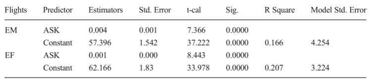
Estimation results from Table6 jointly with Fig.4 show
that there exist weak (coefficients of determinations of 16.6 and 20.7 % respectively) linear relationships be-tween LF and ASK for both EM and EF flights.
There-fore, the closer analysis from Tables 5 and 6 confirm
that relatively the airliners have better demand manage-ment than capacity managemanage-ment for the EM and EF flights.
4.2 Assessment of the structure of autocorrelation of load factors (LF)
The correct autocorrelation structure for time series analysis is challenging. However, one powerful method for identification is the spectral density analysis. The spectral density is a non-parametric analysis able to give graphical information about how the autocorrelation function behaves in Fourier space.
One of the main graphical methods of spectral density es-timation is the response of periodogram for the autocorrelation function frequency of the time series data. This method is extremely sensitive to the optimal autocorrelation structure. Another major method for spectral density estimation is the response of density for the autocorrelation function frequency of the time series data. This method is sensitive to the weight-ed autocorrelation structure of the data. Therefore, both fre-quency plots have important information about the autocorre-lation structure for the load factor. The result of the non-parametric spectral density estimation and the non-parametric
Ljung–Box test of the load factors of the EM and EF flights
is given in Table7.
The estimation of the periodogram and spectral den-sity for the LF for the EM flights suggests that there exists strong periodic autocorrelation. The periodic au-tocorrelations are observed after jumping a specific number of months. The yearly repetitive plot of LF of the EM flights over months indicates that there are pe-riodic dependencies. That is the monthly configured
pat-terns for the EM flight’s load factor shows some
regu-larity. The smallest LF is observed in May growing until August every year. Once it reaches its peak in August, it starts to decline until November. From No-vember to April the next year the load factor show a stable growth. The cycle stops when the load factor suddenly drops from April to May to find its minimum. The plots for the periodogram and the spectral density suggest that the LF distribution of the EM flight has serial correlation up to a certain number of lags in months. The Ljung-Box test detect that the LF is seri-ally correlated with the order of 15 months and dissi-pated after 16th month.
The periodogram and the spectral density of the load factor for the EF flights indicate strong periodic auto-correlation. The periodic autocorrelations are observed after a specific number of months. The yearly repetitive
Table 6 Prais-Winsten recursive
parameter estimation of a linear regression of Load Factor (in percentage) in response to ASK (in million)
Flights Predictor Estimators Std. Error t-cal Sig. R Square Model Std. Error
EM ASK 0.004 0.001 7.366 0.0000
Constant 57.396 1.542 37.222 0.0000 0.166 4.254
EF ASK 0.001 0.000 8.443 0.0000
Constant 62.166 1.83 33.978 0.0000 0.207 3.224
plot over months suggests that there are strong periodic dependencies. As for the EM flights, the monthly-configured patterns of LF of the EF flights show some regularity. As for the EM flights the smallest LF is observed in May growing until August. After reaching its peak in August it starts to decline until December. From December to January the following year the load factor show a growth. The cycle stops when the load factor drops from January to May to find its minimum. The plots of the periodogram and the spectral density
suggest that the LF distribution of the EF flight has serial correlation for several months. The Ljung-Box test statistic detects that the LF is serially correlated with the order of 13 months and dissipated after 14th month.
4.3 Fitting load factors using a multivariate trend model
The analyses above recognise that both the RPK and ASK for the EF flights are higher than for the EM flights. Similarly, the average LF for the EF flights is higher than for the EM flights. Moreover, above we a l s o f o u n d t h a t t h e L F h a s d i ff e r e n t e c h e l o n s (magnitudes) of linear correlation with RPK for the EM and EF flights. Besides, the analyses prevails that the linear correlation of LF with ASK is weak for both flights. Therefore, using these variables (both RPK and ASK) as common exogenous cohorts for the prediction of the load factor is inappropriate. Therefore, we can explicitly fit the trend model of the EM flight and the EF flight. We are only left with time as a predictor of LF for both flights. Thus, rather than other models, for example panel data regression model, we apply multi-variate trend models.
The analyses of the autocorrelation structure have shown that both periodic and serial correlations exist for the LF. More importantly, the structure of autocor-relation is different for two flights. This is showing that Fig. 4 Scatter Plot of load factor (in %) ASK (in million)
Table 7 The structure of autocorrelation of load factor of EM and EF flights of airlines under the AEA
Regions Monthly distributions of load factor
across regions over time
Autocorrelation structure of load factor using Periodogram
Autocorrelation structure of load factor using Density
Ljung-Box Q
Chi-Sq DF Sig.
EM
Flights
122.41 15 .000
EF
Flights
13
the time effect on the LF is not simply fixed or random effects; rather it is dynamic and uniquely associated with the regional flights. Therefore, we will use tran-scendental time functions as LF predictors to control for periodic autocorrelation in our multivariate trend model. The fit of the multivariate trend model of the
LF of the EM and EF flights is given in Table 8. The
significance of the harmonic time function confirms the seasonality LF for the EM and EF flights. The
signifi-cance of time (t) for the fitted model suggests that the
LF is improving (growing) with time for both flights. However, the significance of the natural logarithm of
time (ln (t)) in the model for the EF flights suggests
that the LF performances improvements of the airlines are better for the EF flights than for the EM flights.
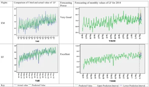
In Fig. 5 (left side) we report the comparison of the
actual and the predicted values for the load factors. From the Figure we can see that the fit of the multivar-iate trend model is found to be robust and realistic for the load factor forecast of both flights. Furthermore, in
Fig. 5 (right side) we give the plots of the monthly
forecasted LF values with upper and lower 95 % pre-diction intervals for the year 2014.
5 Conclusions and recommendations
5.1 Conclusions
This study applied advanced econometric analysis on the load factor (LF) of flights of Europe-Middle East (EM) and Far East (EF) of Association Europe-an Airlines (AEA). The econometric Europe-analysis provides the following conclusions. The mean RPK for the EM and EF flights are 1696.92 and 9671.81 million, respec-tively. Likewise, the mean ASK for the EM and EF are 2450.76 and 12,375.32 million, respectively. Therefore, both in airline transportation demand and capacity the EF flights are higher than for the EM flights. However, the average LF of the EM flights is 9.094 % higher than for the EF flights.
Table 8 The fits of multivariate trend model of the load factor of EM and EF flights
Parameter Estimates Components offi(t;βi) Estimates Std. Error t-cal Approx.
Significance
Model Std. Error
Forecasting of Load factor of 2014 (in %)
Month Expected LB UB
Rho (AR1-EM) 0.47065 0.05403 8.7109 0.00000 3.10843 Jan 68.48439 62.36979 74.59898 Time function Coefficients t 0.04047 0.00440 9.2040 0.00000 Feb 70.82609 64.7115 76.94069
Sin(ω2t) −0.89069 0.23959 −3.7176 0.00025 Mar 73.48739 67.37279 79.60199
Sin(ω3t) 1.56918 0.30565 5.1340 0.00000 Apr 75.61921 69.50461 81.7338
Sin(ω6t) −2.44483 0.41552 −5.8838 0.00000 May 71.20958 65.09498 77.32418
Cos(ω1t) 0.66278 0.12738 5.2032 0.00000 Jun 73.23854 67.12394 79.35313 Cos(ω2t) 2.19048 0.23959 9.1428 0.00000 Jul 78.23464 72.12004 84.34924
Cos(ω3t) −2.05430 0.30510 −6.7332 0.00000 Aug 82.73358 76.61898 88.84817
Cos(ω6t) −3.04910 0.41357 −7.3726 0.00000 Sep 76.83852 70.72392 82.95312 Constant of EM Flights 62.35790 0.70356 88.6320 0.00000 Oct 72.66656 66.55196 78.78115 Nov 70.39743 64.28283 76.51203 Dec 71.76413 65.64953 77.87873 Rho (AR1-EF) 0.5381 0.0507 10.603 0.0000 2.278 Jan 81.15884 76.67778 85.63989 Time function Coefficients t 0.0250 0.0074 3.3849 0.0008 Feb 84.1656 79.68454 88.64665 ln(t) 2.4256 0.5892 4.1171 0.0001 Mar 84.06061 79.57955 88.54167
Sin(ω2t) −0.8707 0.1710 −5.093 0.0000 Apr 80.45579 75.97473 84.93685
Sin(ω3t) 2.1558 0.2242 9.6166 0.0000 May 78.56003 74.07897 83.04109
Sin(ω6t) −2.4322 0.3252 −7.480 0.0000 Jun 81.36409 76.88303 85.84515
Cos(ω2t) −0.3753 0.1709 −2.196 0.0289 Jul 85.53465 81.05359 90.01571
Cos(ω3t) −2.1171 0.2235 −9.471 0.0000 Aug 87.12244 82.64139 91.6035
The LF for both EM and EF flights are significantly positive correlated with both the RPK and ASK. This generally showed that the airlines have good reaction strategy to their demand. More importantly, we found significant correlation of LF with RPK for the EM and EF flights. However, the significance of correlation of LF with ASK is weak for the EM and EF flights. This confirms that the airlines have better demand than capacity management system for both the EM and the EF flights.
The LF of both EM and EF flights has periodic (season-to-season) correlations. The smallest LF for EM flights is ob-served in November, December and January then started to grow until July, August and September, and then declining until November. The smallest LF of EF flights is observed in January then it started grow until July, and then declining until December. Furthermore, the LF of both EM and EF flights has serial (month to month) correlations. The LF of EM and EF flights have correlation order of 15 and 13 months, respectively.
Since we have no common exogenous input for the EM and EF flights, we fit multivariate trend model. Using the fitted model we have given forecasted the monthly values for the LF with upper and lower 95 % prediction intervals for 2014.
5.2 Recommendations and policy implications
This paper has applied econometric models to analyse the LF of EM and EF flights of airlines of the AEA.
Our results have important managerial policy implica-tions and may suggest the following policy recommen-dations. Fit of the LF using the multivariate time series model is found more robust and realistic. The AEA may therefore use the model for prediction of the LF for the distribution of relevant flights. Hence, it is rec-ommended that the AEA apply the model to regional flights. In the airline industry, in addition to decreasing the airlines cost, the profitability of a given airline is dependent on the joint maximization of yield and LF. In order to push up the LF and the yield simultaneous-ly, and to produce strategic decisions about the profit-ability of airlines, the AEA may extend the LF analy-sis to individual airlines. The outcome of such analyanaly-sis will give rigorous information about the LF. Conse-quently, the AEA will have quantitative input on how to restructure the yield management, network design, etc. with respect of specific flights over time. The econometric analysis have identified that the demand management of the airlines is better than the capacity management. In this regard, the AEA is recommended to keep up with the existing demand management strat-egy and improvement is needed on the stratstrat-egy of ca-pacity management. Finally, as suggested by many in-ternational industry studies, the airline industry is sea-sonal. In this paper, we find that the LF of the EM and EF flights are both seasonal and differ between flights. The result implies that the LF is far from stable and
Flights Comparison of f itted and actual value of LF Forecasting Power
Forecasting of monthly values of LF for 2014
EM
Very Good
EF
Excellent
Key Actual value Predicted Value Predicted Value Upper Prediction Interval Lower Prediction Interval
stabilizing policies by airlines has so far not been suc-cessful. The AEA may therefore continuously focus on the stabilisation and the improvement of the LF for the industry.
Acknowledgments First of all we have ultimate thank for God, who
gave us space to live and time to think. Secondly, we would like to thank all the members of the Made University College. Finally, we want to thank all the scholars referenced in the paper.
Open AccessThis article is distributed under the terms of the Creative Commons Attribution License which permits any use, distribution and reproduction in any medium, provided the original author(s) and source are credited.
References
1. Amemiya T (1985) Advanced econometrics. Harvard University Press, Cambridge
2. Baltagi BH (2008) Econometric analysis of panel data, 4th edn. John Wiley & Sons, Chichester
3. Boashash B (2003) Time-frequency signal analysis and processing: a comprehensive reference. Elsevier Science, Oxford
4. Brueckner JK, Whalen WT (2000) The price effects of international airlinealliances. Journal of Law and Economics 43:503–545 5. Chan J, Koop G, Leon-Gonzales R, Strachan R (2012) Time varying
dimension models. J Bus Econ Stat Vol 30
6. Cochran WG, Cox GM (1992) Experimental designs, 2nd edn. Wiley, New York
7. Cook RD, Weisberg S (1982) Residuals and influence in regression, Reprth edn. Chapman and Hall, New York
8. Cross RG (1997) Revenue management: hard-core tactics for market domination. Broadway Books, New York
9. Cross R, Higbie J, Cross Z (2010) Milestones in the application of analytical pricing and revenue management. J Rev Pricing Manag 10: 8–18
10. Davidson J (2000) Econometric theory. Blackwell Publishing, Oxford, UK
11. Davidson R, Mackinnon JG (1993) Estimation and inference in econometrics. Oxford University Press, Oxford
12. Davies A, Lahiri K (1995) A new framework for testing rationality and measuring aggregate shocks using panel data. Journal of Econometrics 68:205–227
13. Davison AC, Hinkley DV (1997) Bootstrap methods and their appli-cations. Cambridge University Press, Cambridge
14. Distexhe V, Perelman S (1994) Technical efficiency and productivity growth in an era of deregulation: the case of airlines. Revue Suisse d’Economie Politique 130(4):669–689
15. Doganis R (2010) Flying off course, airline economics and market-ing, 4th edn. Routledge, LonMAn and New York
16. Engelberg S (2008) Digital signal processing: an experimental ap-proach. Springer, ISBN 978-1-84800-118-3
17. Fahrmeir L, Kneib T, Lang S (2009) Regression. Model and method, 2nd edn. Springer, Heidelberg
18. Flores-Fillol R, Moner-Colonques R (2007) Strategic formation of airline alliances. Journal of Transport Economics and Policy 41(3): 427–449
19. Frees E (2004) Longitudinal and panel data: analysis and applications in the social sciences. Cambridge University Press, New York 20. Hamilton JD (1994) Time series analysis. Princeton University Press 21. ICAO (2013) Airport Economics Manual: Retrieved on 21 April 2014 at:www.icao.int/sustainability/MAcuments/MAc9562_en.pdf
22. Kahn AE (1988) Surprises of deregulation. The American Economic Review 78(2):316–322, JSTOR
23. Kammler D (2000) A first course in Fourier analysis. Prentice Hall, Upper Saddle River
24. Karagiannis E, Kovacevic M (2000) A method to calculate the jack-knife variance estimator for the Gini coefficient. Oxford Bulletin of Economics and Statistics 62:119–122
25. Kaul S (2009) Yield management: getting more out of what you already have. Ericsson Business Review, No. 2: 17–19
26. Link H (2004) PEP-a yield-management scheme for rail passenger fares in Germany. Japan Railway & Transport Review 38:54 27. Kellner L (2000) Building a global airline brand, 2000 Transport
Conference. UBS Warburg, London
28. Luc B, Lubrano M, Jean-François R (2000) Bayesian Inference in Dynamic Econometric Models Oxford Scholarship Online: October 2011
29. Lütkepohl H (2006) New introduction to multiple time series analy-sis. Springer, Berlin
30. Marriott JJ, Cross RG (2000) Room at the revenue inn. In: Krass P (ed) Book of management WisMAm: classic writings by legendary managers. Wiley, New York, pp 199–208
31. McGill J, Van Ryzin G (1999) Revenue management: research over-view and prospects. Transportation Science 33:233–256
32. Minho C, Ming Fan, Yong-Pin Z (2007) An Empirical Study of Revenue Management Practices in the Airline Industry, Michael G. Foster School of Business University of Washington
33. Netessine S, Shumsky R (2002). Introduction to the Theory and Practice of Yield Management. INFORMS Trans Educ 3:(1) 34. Prais SJ, Winsten CB (1954) Trend estimators and serial correlation.
Cowles Commission, Chicago
35. Priestley MB (1991) Spectral analysis and time series. Academic, New York
36. Stoica P, Moses R (2005) Spectral analysis of signals. Prentice Hall, Upper Saddle River, 07458
37. Talluri KT, Van Ryzin GJ (2001) Revenue management under a gen-eral discrete choice model of consumer behavior. Manag Sci 38. Talluri KT, Van Ryzin GJ (2004) The theory and practice of revenue
management. Kluwer Academic Publishers, Norwell, Massachusettes 39. Kailath T, Sayed AH, Babak H (2000) Linear Estimation.
Prentice-Hall
40. Van Dender K (2007) Determinants of fares and operating revenues at US airports. J Urban Econ 62:317–336
41. Vassilis AH (2008) Computational methods in econometrics. The New Palgrave Dictionary of Economics, 2nd Edn
42. Verbeek M (2004) A guide to modern econometrics, 2nd edn. John Wiley & Sons, Chichester
43. Weisberg S (1985) Applied linear regression, 2nd edn. Wiley, New York