https://doi.org/10.5194/ms-9-81-2018
© Author(s) 2018. This work is distributed under the Creative Commons Attribution 4.0 License.
Modelling, simulation and experiment
of the spherical flexible joint stiffness
Songyu Li1, Liquan Wang1, Shaoming Yao2, Peng Jia1, Feihong Yun1, Wenxue Jin1, and Dong Lv1
1College of Mechanical and Electronical Engineering, Harbin Engineering University, Harbin, 150001, China
2AMRC with Boeing, the University of Sheffield, Sheffield, S60 5TZ, UK
Correspondence:Liquan Wang ([email protected])
Received: 11 September 2017 – Revised: 5 January 2018 – Accepted: 1 February 2018 – Published: 19 February 2018
Abstract. The spherical flexible joint is extensively used in engineering. It is designed to provide flexibility in rotation while bearing vertical compression load. The linear rotational stiffness of the flexible joint is formulated. The rotational stiffness of the bonded rubber layer is related to inner radius, thickness and two edge angles. FEM is used to verify the analytical solution and analyze the stiffness. The Mooney–Rivlin, Neo Hooke and Yeoh constitutive models are used in the simulation. The experiment is taken to obtain the material coefficient and validate the analytical and FEM results. The Yeoh model can reflect the deformation trend more accurately, but the error in the nearly linear district is bigger than the Mooney–Rivlin model. The Mooney–Rivlin model can fit the test result very well and the analytical solution can also be used when the rubber deformation in the flexible joint is small. The increase of Poisson’s ratio of the rubber layers will enhance the vertical compression stiffness but barely have effect on the rotational stiffness.
1 Introduction
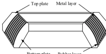
The spherical flexible joints are widely used as non-rigid connection in aerospace and offshore oil and gas industry. The flexible joint is the critical part of the flexible bearing nozzle in the solid rocket boosters (SRB). It allows nozzle to deflect in given directions for booster thrust vector control (Kumar et al., 2015). Elastomeric bearings are flexible joints used in helicopter rotor hubs. These bearings are spherical hinges to withstand centrifugal and lateral forces while toler-ating rotational, flap and lead-lag motions (Donguy, 2015). In the offshore oil and gas industry, the flex joints, also known as FlexJoints®, are used to connect TLP (tension leg plat-form) to the subsea foundation (Kumar, 2000). A typical flex-ible joint consists of alternately laminated spherical rubber and metal layers. For different application, the configuration of the metal layers may be slightly different. The metal layers of rocket solid booster flexible bearings may protrude outside the rubber layers to resist to higher temperature (Lampani et al., 2012). On the contrary, to protect the metal from sea-water corrosion, the metal layers of FlexJoints®are wrapped in the rubber layer (Gunderson et al., 1992).
Metal layer
Rubber layer Bottom plate
Top plate
Figure 1.Typical flexible joint.
strips based on two kinematic assumptions and one stress as-sumption:
a. planes parallel to the rigid surface will keep plane and parallel during or after deformation;
b. lines normal to the rigid surface will be changed to parabolic after deformation produced by the compres-sion;
c. normal stress components in three directions are equal to the mean pressure.
The rubber block in this approximation is assumed incom-pressible, which will overestimate the compression stiffness when the shape factor is high. Therefore, another method was proposed with regard of bulk compressibility (Chalhoub and Kelly, 1990, 1991; Kelly, 1993). The method applies to the rubber layers of circular, infinite-strip and square shapes with Poisson’ ratio between 0.49 and 0.5. Tsai and Pai proposed a new method for the full range of Poisson’s ratio with two kinematic assumptions to calculate the effective compression moduli of the rubber layers with infinite-strip, circular and square shapes (Tsai and Lee, 1998). Wang et al. (2017) used the same method to calculate the effective compression mod-ulus of the spherical bonded rubber layer.
The flexible joint undergoes pure shear deformation under the torsional moment. Some studies have been taken on the shear deformation of the rubber bearings with circular and square shapes (He et al., 2012; Mishra and Igarashi, 2013). Exact closed-form expressions are derived for the torsional stiffness of the spherical rubber bush mountings (Horton and Tupholme, 2005). Zhang et al. (2012) used nonlinear FEM to simulate the SRB flexible joint structural behaviour and conducted experiments to validate the analysis. But the stiff-ness was not studied. Chen and Yang (2015) proposed an an-alytical method to calculate the compression and torsional stiffness of the helicopter rotor elastomeric bearings with in-compressible assumption. An experiment was conducted to validate the analytical solution. But the calculation error is too big.
The linear vertical stiffness of the spherical bonded rubber layer has been presented in the previous work (Wang et al., 2017). A closed-form expression of the linear rotational stiff-ness of the bonded rubber layer is proposed. The influence
Metal layer
Parabolic form
Rubber layer
Figure 2.The parabolic form of rubber boundary.
factors on the rotational stiffness are studied. FEM is used to verify the analytical result and analyse the stiffness of the flexible joint. The experiment is taken to validate the simula-tion and analytical results.
2 Formulation of the linear stiffness
The sectional view of a typical flexible joint is shown in Fig. 1. It is spherical and consists of laminated rubber and metal layers. The top plate is fixed and loads are applied to the bottom plate. Generally, the spherical rubber and metal layers are equivalent to be in series and have a coincident centre. Thus the total linear stiffness,K, of the flexible joint could be calculated by the expression below:
K=
X 1
Ki
−1
, (1)
whereKi is the vertical compression stiffness (or rotational stiffness) of the rubber layeri.
Some assumptions are given to calculate the linear vertical compression stiffness and rotational stiffness of the flexible joint:
a. the metal layer is rigid;
b. planes parallel to the metal layer will remain plane and parallel during or after compression deformation;
c. lines normal to the metal layer will be changed to parabolic after the deformation produced by the com-pression loads, as shown in Fig. 2.
2.1 Vertical compression stiffness
y z
O
ti
Ri
φ1i
φ2i
Restrained surfaces
Free surfaces Median layer
x
Figure 3.A single rubber layer of the flexible joint.
Kc=
4π(R+t /2)2G(x1−x2)−
2π(R+t /2)2Gv kεc(1−2v)
x2
Z
x1
C1Pd(x)+C2Qd(x)+k(εc−δεc)dx
cos2ϕ e
t , (2)
whereGandvare respectively the initial shear modulus and Poisson’s ratio of the rubber; R andt are respectively the inner radius and thickness of the rubber layer;kis the volume modulus, εc is the effective compression strain; Pd(x) and Qd(x) are respectively Legendre function of the 1st and 2nd
kind;d=1
2
q
1+2α11−−ν2ν −1
2 is the degree of the function; δεc= −2(3tR(32R++32Rt+tt)εc2); x1=cotϕ1,x2=cotϕ2; ϕe=(ϕ1+ ϕ2)/2.
C1= C3 C4
kα
4(x21−1)(x22−1) δ−ν 1−νεc,
C2=
−C1
αPd(x1) 2 +
x1(d+1)[x1Pd(x1)−Pd+1(x1)] x12−1
+k 2
h
1−2ν
1−ν (1−δ)+2δ−1
i
εc
αQd(x1)
2 +
x1(x1+1)[x1Qd(x1)−Qd+1(x1)] x22−1
,
C3=(x22−1)
h
α(x12−1)+2x12(d+1)
i
Qd(x1) −(x12−1)hα(x22−1)+2x22(d+1)iQd(x2)
+2(d+1)h(x12−1)x2Qd+1(x2)−(x22−1)x1Qd+1(x1)
i
,
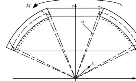
y z
O α
x M
Figure 4.The boundary conditions and loading of rotational rubber layer.
C4=
(
αQd(x1)
2 +
x1(d+1)[x1Qd(x1)−Qd+1(x1)] x21−1
)
·
(
αPd(x2)
2 +
x2(d+1)[x2Pd(x2)−Pd+1(x2)] x22−1
)
−
(
αPd(x1)
2 +
x1(d+1)[x1Pd(x1)−Pd+1(x1)] x12−1
)
·
(
αQd(x2)
2 +
x2(d+1)[x2Qd(x2)−Qd+1(x2)] x22−1
)
α=1 R(R+t) t(2R+t)ln
R+t
R −
1 2
.
2.2 Rotational stiffness
Because the rubber layer is axisymmetric aboutzaxis, the
rotational stiffness about any axes which pass through the origin inxyplane will be the same. The linear rotational stiff-ness about thex axis is calculated by semi-inverse method. As shown in Fig. 4, the bottom is fixed and a torsional mo-ment,M, is applied to the top surface. An angle,α, around x axis is produced in the rubber layer. Only shear deforma-tion occur when the thickness is much smaller than the in-ner radius, so there is no deformation alongr direction and u(r)=0. Any point in the rubber layer moves along a circle of radius (y2+z2)0.5centered on thexaxis and the
displace-ment parallel toxaxis is zero. In that case, for any point on zyplane (θ=90◦), the displacement in theϕdirection only related toranduϕ=V1(r), the displacement in theθ
the above conditions, the displacement components are as-sumed as below:
ur=0, (3)
uϕ=V(r) sinθ, uθ=V(r) cosϕcosθ,
whereV(r) is the function ofr. Because Poisson’s ratio has a low influence on the rotational stiffness, the rubber is as-sumed as completely incompressible here. Thus the volume modulus is infinite andεrr+εϕϕ+εθ θ=0.According to the displacement assumption, the strain in the rubber layer can be calculated as
εrr=εϕϕ=εθ θ =εθ ϕ=εϕθ=0,
εrϕ=εϕr = 1 2
dV(r)
dr −
V(r) r
sinθ,
εrθ =εθ r= 1 2
dV(r)
dr −
V(r) r
cosθcosϕ. (4)
According to the Hooke law, the stress is
σrr=σϕϕ=σθ θ,
σrϕ=σϕr=G
dV(r)
dr −
V(r) r
sinθ,
σrθ =σθ r=G
dV(r)
dr −
V(r) r
cosθcosϕ,
σθ ϕ=σϕθ=0. (5)
Thus the equilibrium equations of the rubber layer in spher-ical coordinate system (Landau and Lifshitz, 1986) can be expressed as
∂σϕϕ ∂r =0, ∂σϕϕ
∂θ +G
rd 2V dr2 +2
dV dr −2
V r
sinϕcosϕcosθ=0,
∂σϕϕ
∂ϕ +G
rd 2V dr2 +2
dV
dr −2 V
r
sinϕ=0. (6)
According to the first equation in Eq. (6),σϕϕ is not related tor.rd2V
dr2 +2 dV dr −2
V
r needs to be 0 if the latter two equa-tions in Eq. (6) validate for anyϕandθ. Then the latter two
equations become ∂σϕϕ/∂θ=0 and∂σϕϕ/∂ϕ=0. So, the
general solution of the equations is
σϕϕ=C1,
V(r)=C2r+C3/r2, (7)
whereC1,C2,C3are constants.
To make the results more general, define a parameter r=R+s,s∈ [0, t]. The boundary condition on the free sur-faces of the rubber layer can be approximately expressed as
σϕϕ=σθ θ=σrr=C1=0 whenϕ=ϕ1andϕ=ϕ2.
Substi-tute Eq. (7) into Eq. (5) and yield
σrϕ=σϕr= − 3GC3
(R+s)3sinθ, σrθ=σθ r= −
3GC3
(R+s)3cosθcosϕ. (8)
The torsional momentMcan be expressed by the stress inte-gration as
M= −
2π
Z
0
ϕ2
Z
ϕ1
(R+s) sinϕsinθ(−sinϕσϕr)
−(R+s) cosϕ(cosϕsinθ σϕr+cosθ σθ r)
(R+s)2sinϕdϕdθ. (9)
Substitute Eq. (8) into Eq. (9) and yield
C3= −
M
π G[(3 cosϕ1+cos3ϕ1)−(3 cosϕ2+cos3ϕ2)]
. (10)
The boundary condition on the restrained surfaces of the rub-ber layer can be expressed as
uθ=uϕ=0, s=0, (11)
(uϕcosϕsinθ+uθcosθ)
(R+t) cosϕ
D +(uϕsinϕ) (R+t) sinθsinϕ
D =αD, s=t, (12)
whereD=(R+t)psin2θsin2ϕ+cos2ϕ, which is the
dis-tance between a point on the top restrained surface and xaxis.
Substitute Eqs. (3) and (7) into Eq. (12) and yield
C2= − C3 R3 =
(R+t)3
(R+t)3−R3α. (13)
Thus the rotational stiffnessKri of the rubber layeriis
Kri= Mi
αi
=π G R 3
i(Ri+ti)3 (Ri+ti)3−R3i
(3 cosϕ1i+cos3ϕ1i)
−(3 cosϕ2i+cos3ϕ2i)
. (14)
Because the rubber thicknessti is far less than the rubber layer radiusRi, defineρi=ti/Ri andρi 0.Then Eq. (14) will be simplified as
Ki ≈π G
Ri6(1+3ρi) Ri3(3ρi)
3 cosϕ1i+cos3ϕ1i
− 3 cosϕ2i+cos3ϕ2i
=π GR3i
1
3ρi
+1 3 cosϕ1i+cos
3ϕ 1i
− 3 cosϕ2i+cos3ϕ2i
0.3 0.4 0.5 0.6 0.7 0.8 0.9 1.0 1.1 1.2 1.3 0
4 8 12 16
Edge angle (rad)
R
ot
at
io
na
l s
tif
fn
es
s
(N
m
r
ad
-1)
Variation of the inner edge angle Variation of the outter edge angle
×104
Figure 5.Rotational stiffness variation along with edge angles.
3 Rotational stiffness analyses
The vertical compression stiffness of the bonded rubber layer has been analyzed in Wang et al. (2017), here the rotational stiffness will be analyzed. According to Eqs. (5) and (7), the rubber layer bears pure shear stress in rotation and the rota-tional stiffness is proporrota-tional to the shear modulus. Besides the shear modulus, the rotational stiffness is also related to the inner radius, the thickness and two edge angles. A bonded rubber layer is modelled to analyze the rotational stiffness by individual variables. Its inner radius, R, is 100 mm; the thickness,t, is 2 mm; the edge angles of free surfaces,ϕ1and ϕ2, are, respectively, 20 and 70◦. Because the rubber
thick-ness is far less than the radius, which is the displacement assumption, the analytical result will be inaccurate when the thickness-radius ratio is rather low.
Figure 5 shows the relation between the rotational stiffness and the edge angles. When the outer edge angle is constant the rotational stiffness decreases if the inner edge angle in-creases and when the inner angle is constant it inin-creases if the outer edge angle increases. The trend is approximately linear when edge angles are between 0.3 and 1.3 rad.
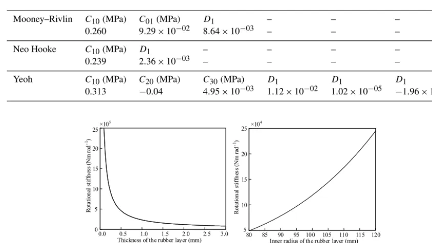
Figure 6a shows the relation between the rotational stiff-ness and the thickstiff-ness of the rubber layer. The curve is a hy-perbola. When the thickness approaches to zero, the stiffness approaches to infinite. As the thickness increases from 0 to 0.5 mm, the stiffness decreases sharply. Then the stiffness de-creases gently. Figure 6b shows the relation between the ro-tational stiffness and the inner radius of the rubber layer. It can be seen the rotational stiffness increases as the inner ra-dius increases. Comparing Fig. 6a and Fig. 6b, decreasing the thickness of the rubber layer will be more effective to increase the rotational stiffness when the overall size of the rubber layer is constant.
4 Simulation and experiment
A prototype of the flexible joint is manufactured, as shown in Fig. 7. The flexible joint consists of four rubber layers.
Table 1.Geometric parameters of rubber layers.
No. of Inner Thickness Inner Outer
rubber radius (ti)/mm edge edge
layer (i) (Ri)/mm angle angle
(ϕ1i)/◦ (ϕ2i)/◦
1 140 3 42.4 74.6
2 150 4 42.6 71.2
3 161 4 42.7 68.2
4 172 3 42.9 65.8
Three metal layers are evenly arranged and fully wrapped by the rubber. The thickness of the inner and outer rubber on the edge of the flexible joint is 3 mm. The thickness of the metal layer is 7 mm. The specific geometric parameters of every rubber layers are shown in Table 1. A static nonlinear anal-ysis is taken on the flexible joint in Abaqus/Standard. The stress of the flexible joint under compression is axisymmet-ric, so a 2-D FE model is enough for the simulation. A half 3-D joint model can be used to simulate the flexible joint
un-der torsional moment which is symmetric aboutxyplane.
The linear elastic material model is applied to the metal layers. The property coefficients of the metal layers are
Young’s modulusE=206 GPa and Poisson’s ratiov=0.3.
The rubber is modeled by the hyperelastic material model. The relation between stress and strain is derived from a strain energy density function. The Mooney–Rivlin, Neo Hooke and Yeoh constitutive models are used in this simulation.
The Nitrile rubber reinforced by carbon-black is used in the flexible joint prototype. Figure 8a shows the test data of the uniaxial tension test of the rubber. The test was per-formed on dumbbell shaped specimens prepared according to Type 1A GB/T 528-2009. The test was carried out on the tensile testing machine. The interested strain range is 0– 200 % in the rubber of the flexible joint. The rubber material is nearly incompressible, which means its bulk modulus is far larger than shear modulus and Poisson’s ratio is close to 0.5. In the simulation of the rubber with tensile and shear de-formation, Poisson’s ratio is always assumed to be 0.5 and then bulk modulus goes to infinite. But that will overestimate the compression capacity of the rubber component when it is highly constrained and compressed. Thus the measuring of the incompressible parameter D1is necessary. It equals
Table 2.Coefficients of constitutive model.
Mooney–Rivlin C10(MPa) C01(MPa) D1 – – –
0.260 9.29×10−02 8.64×10−03 – – –
Neo Hooke C10(MPa) D1 – – – –
0.239 2.36×10−03 – – – –
Yeoh C10(MPa) C20(MPa) C30(MPa) D1 D1 D1
0.313 −0.04 4.95×10−03 1.12×10−02 1.02×10−05 −1.96×10−07
80 85 90 95 100 105 110 115 120 5
10 15 20 25
R
ot
at
io
na
l s
tif
fn
es
s
(N
m
r
ad
-1)
Inner radius of the rubber layer (mm) ×104
0.0 0.5 1.0 1.5 2.0 2.5 3.0 0
5 10 15 20 25
R
ot
at
io
na
l s
tif
fn
es
s
(N
m
r
ad
-1)
Thickness of the rubber layer (mm) ×105
(a) Rotational stiffness variation along with thickness (b) Rotational stiffness variation along with inner radius
Figure 6.Rotational stiffness variation along with thickness and inner radius.
170
85
Figure 7.Detailed dimension of the flexible joint.
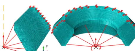
The increment is fixed as 0.1 in all steps in the simulation. The nlgeom option is on. As shown in Fig. 9, the top plate of the flexible joint is fixed. A reference point RP-1 is set at the coincident center. The reference point is coupled with the bottom plate of the flexible joint in the interaction module. A displacement of 2.5 mm iny is set on the reference point in the 2-D analysis. An angle of 0.15 rad in zaxis is set on the reference in both steps in the 3-D analysis. Meanwhile the symmetry boundary condition is also applied in the 3-D model.
The meshes of models are shown in Fig. 9. For nearly incompressible materials, hourglassing and volume locking phenomena may occur during simulation. Thus the hybrid and second-order elements are used to solve these prob-lems. The 2-D axisymmetric element, CAX8R, is used for the metal part and CAX8RH is used for the rubber part in 2-D model. The 3-D solid element, C3D20R, is used for the
metal part and C3D20RH is used for the rubber part in 3-D model.
To validate the theoretical and simulation results, a test de-vice was designed to carry out the compression and rotation test for the prototype, as shown in Fig. 10. The compression and rotation loading was provided by a 2000 kN compres-sion tester. Four 500 kN pressure sensors were used in paral-lel to measure the loading. A laser displacement sensor and an angle sensor were respectively used in compression and rotation test. In the compression test, the flexible joint was directly compressed by the pressure tester. The maximum compression loading is set as 1000 kN. The loading speed is about 40 kN min−1. In the rotation test, the loading was trans-mitted from the tester to the flexible joint by a turning stick. There are two hinges on the stick, so the pressure loading will be always perpendicular to the bottom plate of the
flex-ible joint. The maximum rotation angle was about 8◦. The
loading speed was about 3◦min−1. Both tests were repeated 5 times.
5 Results and discussions
5 10 15 20 25 30 0
2 4 6 8 10 12 14 16
T
en
si
le
l
oa
di
ng
(
N
)
Tensile displacement (mm)
(a) Uniaxial tension test data (b) Volumetric compression test data
0.90 0.91 0.92 0.93 0.94 0.95 0.96 0.97 0.98 0.99 1 0
20 40 60 80 100 120 140
P
re
ss
ur
e
(
M
pa
)
Volume ratio
Figure 8.Test data of the flexible joint rubber.
RP-1 x
y
RP-1
Figure 9.FE mesh of the flexible joint models.
trend of the flexible joint, but its error in the nearly linear dis-trict is bigger than the Mooney–Rivlin model and that error increases rapidly as the compression displacement increases. Thus the Mooney–Rivlin model is used to calculate the linear vertical compression stiffness of the flexible joint. Accord-ing to the Mooney–Rivlin material coefficient in Table.2, the initial shear modulus is 0.706 MPa and the Poisson’s ratio is 0.4985. The analytical, FEM and test results of the linear vertical compression stiffness of the flexjoint are respectively 291, 307 and 308 kN mm−1. The error of the analytical result is 5.5 % compared with the test result.
Figure 11b shows the results of the rotation simulation and test. It can be seen that the test curve is almost linear when the rotation angle is smaller than 2◦. Then the rotational stiff-ness of flexible joint decreases. The error of the Neo Hooke model is smaller than the Mooney–Rivlin model in the non-linear district, but they both can not reflect the decrease of the rotational stiffness. The error of the Yeoh model is bigger than the Mooney–Rivlin model in the nearly linear district. But it fits the test result very well in the non-linear district. The result of the Mooney–Rivlin has obvious difference with the test result. But it fits the test result well in the nearly linear district. Thus the Mooney–Rivlin model is used to calculate the linear rotational stiffness of the flexible joint. The analyt-ical, FEM and test results of the linear rotational stiffness of the flexible joint are respectively 441, 468 and 457 Nm per degree. The error of the analytical result is 3.5 % compared with the test result.
After analyzing Fig. 11, it can be considered that the Mooney–Rivlin model can fit the test result very well when
Flexjoint
Pressure sensor Compression
tester Displacement
sensor
Angle sensor
(a) Compression test (b) Rotation test
Turning stick
Figure 10.The compression and rotation test device.
the rubber deformation in the flexible joint is small. The Yeoh model can reflect the deformation trend more accu-rately, but the error in the nearly linear district is bigger than the Mooney–Rivlin model. The analytical solutions are ac-curate in the nearly linear district.
The typical unfilled rubber has Poisson’s ratio in the range of 0.4995 to 0.499995 and filled rubber has Poisson’ ratio in the range of 0.49 to 0.497 (Hibbitt et al., 2016). In order to study the effect of Poisson’s ratio on the flexible joint un-der compression or torsional moment, six FE models with different Poisson’s ratios are created. These Poisson’s ra-tios are 0.49, 0.495, 0.499, 0.4995, 0.4999 and 0.49995 re-spectively. The corresponding incompressible parameters are 0.028, 0.014, 0.0028, 0.0014, 0.00028 and 0.00014 MPa−1.
Figure 12a shows the vertical compression stiffnesses of the flexible joints with different Poisson’s ratios vs. the dis-placement. The analysis is taken in the nearly linear district, which means the maximum displacement is 1.5 mm accord-ing to Fig. 11a. The vertical compression stiffness increases by 3.45 % when Poisson’s ratio is 0.49 and by 8.92 % when Poisson’s ratio is 0.49995. It can be found that as Poisson’s ratio increases, the compression stiffness increases more con-siderably. Besides, as Poisson’s ratio increases from 0.4999 to 0.49995, the compression stiffness tends to be saturated.
anal-I. Nearly linear district
0.0 0.5 1.0 1.5 2.0 2.5
0 200 400 600 800 1000 1200 1400
V
er
tic
al
c
om
pr
es
si
on
(k
N
)
Displacement (mm) (a) Compression test and simulation
Mooney-Rivlin Yeoh Neo Hooke Test
II. Non-linear district
0 1 2 3 4 5 6 7 8
0.0 0.5 1.0 1.5 2.0 2.5 3.0 3.5 4.0
R
ot
at
io
n
m
om
en
t
(k
N
m
)
Angle (°) (b) Rotation test and simulation
Mooney-Rivlin Yeoh Neo Hooke Test
I. Nearly linear district
II. Non-linear district
Figure 11.The FEM simulation and test results.
0.0 0.3 0.6 0.9 1.2 1.5
0 100 200 300 400 500 600 700 800 900
V
er
tic
al
s
tif
fn
es
s
(k
N
m
m
-1)
Displacement (mm)
(a) Compression stiffness-displacement curve v = 0.4995 v = 0.4999 v = 0.49995 v = 0.49
v = 0.495 v = 0.499
0.0 0.5 1.0 1.5 2.0
460 462 464 466 468 470
v = 0.4995 v = 0.4999 v = 0.49995 v = 0.49
v = 0.495 v = 0.499
R
ot
at
io
na
l s
ti
ff
n
es
s
(N
m
/°
)
(b) Rotational stiffness-angle curveAngle (°)
Figure 12.Vertical/rotational stiffness variation along with vertical displacement/angle.
ysis is taken in the nearly linear district, which means the
maximum angle is 2◦according to Fig. 11b. It can be seen
that Poisson’s ratio can barely affect the rotational stiffness. The rotational stiffness also tends to be saturated as Poisson’s ratio increases from 0.4999 to 0.49995.
By comparing two figures in Fig. 12, it can be found that Poisson’s ratio has a more considerable effect on the verti-cal compression stiffness than the rotational stiffness. The vertical stiffness increases by 6.2 times as Poisson’s ratio in-creases from 0.49 to 0.49995. On the contrary, the rotational stiffness only increases by 1.47 % as Poisson’s ratio increases from 0.49 to 0.49995.
6 Conclusions
The analytical formulae of the linear rotational stiffness are derived for the flexible joint. The rotational stiffness of rub-ber layer is related to the inner radius, the thickness and two edge angles. It will decrease when the inner edge angle in-creases and increase when the outer edge angle inin-creases. The increase of the rubber thickness will reduce the rota-tional stiffness. The increase of the inner radius will enhance the rotational stiffness.
The FEM is used to verify the analytical method and ana-lyze the stiffness of the flexible joint. The Mooney–Rivlin,
Neo Hooke and Yeoh constitutive models are used in the simulation. The experiment is taken to obtain the material coefficient and validate the analytical and simulation results. The Yeoh model can reflect the deformation trend more ac-curately, but the error in the nearly linear district is bigger than the Mooney–Rivlin model. The Mooney–Rivlin model can fit the test result very well when the rubber deformation in the flexible joint is small. The error of two analytical so-lutions are respectively 5.5 and 3.5 %. That’s usable in the flexible joint design. The increase of Poisson’s ratio of the rubber layers will enhance the vertical compression stiffness but barely have effect on the rotational stiffness. The vertical stiffness increases by 6.2 times and the rotational stiffness only increases by 1.47 % as Poisson’s ratio increases from 0.49 to 0.49995.
Data availability. The data generated during this study are avail-able from the corresponding author on reasonavail-able request.
Acknowledgements. This research is supported by the National Natural Science Foundation of China (No. 51305088).
Edited by: Lotfi Romdhane
Reviewed by: two anonymous referees
References
Chalhoub, M. S. and Kelly, J. M.: Effect of bulk compressibility on the stiffness of cylindrical base isolation bearings, Int. J. Solids. Struct., 26, 743–760, 1990.
Chalhoub, M. S. and Kelly, J. M.: Analysis of infinite-strip-shaped base isolator with elastomer bulk compression, J. Eng. Mech., 117, 1791–1805, 1991.
Chen, G. S. and Yang, Y.: Stiffness design, simulation and test of laminated spherical elastomeric bearing, Hangkong Dongli Xue-bao/journal of Aerospace Power, 30, 1512–1519, 2015. Crocker, L. and Duncan, B.: Measurement Methods for Obtaining
Volumetric Coefficients for Hyperelastic Modelling of Flexible Adhesives, National Physical Laboratory, Teddington, UK, 2001. Donguy, P.: Development of a helicopter rotor hub elastomeric
bear-ing, J. Aircraft, 17, 346–350, 2015.
Gent, A. N. and Lindley, P. B.: The compression of bonded rubber blocks, P. Inst. Mech. Eng., 173, 111–122, 1959.
Gunderson, R., Stevenson, A., Harris, J., Gahagan, P., and Chilton, T.: Fatigue life of TLP flexelements, Offshore Technol-ogy Conference, 4–7 May 1992, Houston, Texas, USA, 1992. He, W. F., Liu, W. G., Yang, Q. R., and Feng, D. M.:
Non-linear rotation and shear stiffness theory and experiment re-search on rubber isolators, J. Eng. Mech., 138, 441–449, https://doi.org/10.1061/(ASCE)EM.1943-7889.0000350, 2012. Hibbitt, H., Karlsson, B., and Sorensen, P.: Abaqus analysis user’s
manual, Dassault Systèmes Simulia Corp, Providence, USA, 2016.
Horton, J. M. and Tupholme, G. E.: Stiffness of spherical bonded rubber bush mountings, Int. J. Solids. Struct., 42, 3289–3297, https://doi.org/10.1016/j.ijsolstr.2004.10.017, 2005.
Kelly, J. M.: Earthquake-Resistant Design with Rubber, Alden Press, Oxford, England, 1993.
Kumar, A.: Performance-related parameters of elastomeric bear-ings, 9 983 261, The University of Texas at Austin, Ann Arbor, 258 pp., 2000.
Kumar, A. E., Murthy, V. B., Mohan, R. C., and Prakash, D.: Study of Non-Linear Static Behavior of Flex Seal of Rocket Nozzle by Varying Number of Shims, Mater. Today-Proc., 2, 1613–1621, 2015.
Lampani, L., Angelini, F., Bernabei, M., Marocco, R., Fabrizi, M., and Gaundenzi, P.: Finite element analysis of a solid booster flex-ible bearing joint for thrust vector control, Aerotecnica & Spazio, J. Aerospace Sci. Technol. Syst., 91, 53–61, 2012.
Landau, L. D. and Lifshitz, E. M.: Theory of Elasticity, Pergamon Print, Oxford, England, 1986.
Mishra, H. K. and Igarashi, A.: Lateral deformation capacity and stability of layer-bonded scrap tire rubber pad isolators under combined compressive and shear loading, Struct. Eng. Mech., 48, 479–500, https://doi.org/10.12989/sem.2013.48.4.479, 2013. Stevenson, A. and Harris, J.: Fatigue life estimation of flexele-ments for TLP structures, in: Proceedings of the International Conference on Offshore Mechanics and Arctic Engineering, 7– 12 June 1992, Calgary, Alberta, Canada, 241–249, 1992. Tsai, H.-C.: Compression behavior of annular elastic layers bonded
between rigid plates, J. Mech., 28, 657–663, 2012.
Tsai, H.-C. and Lee, C.-C.: Compressive stiffness of elastic layers bonded between rigid plates, Int. J. Solids. Struct., 35, 3053– 3069, 1998.
Wang, L., Li, S., Yao, S., Lv, D., and Jia, P.: Study on the vertical stiffness of the spherical elastic layer bonded be-tween rigid surfaces, Arch. Appl. Mech., 87, 1243–1253, https://doi.org/10.1007/s00419-017-1246-9, 2017.
Zhang, X., Liu, Y., Ren, J., and Zhan, K.: Nonlinear
fi-nite element analysis of the SRM flexible joint, in:
53rd AIAA/ASME/ASCE/AHS/ASC Structures, Structural