Physically motivated global alignment method for electron tomography

R E S E A R C H

Open Access

Physically motivated global alignment method

for electron tomography

Toby Sanders

, Micah Prange

, Cem Akatay

and Peter Binev

Abstract

Electron tomography is widely used for nanoscale determination of 3-D structures in many areas of science. Determining the 3-D structure of a sample from electron tomography involves three major steps: acquisition of sequence of 2-D projection images of the sample with the electron microscope, alignment of the images to a common coordinate system, and 3-D reconstruction and segmentation of the sample from the aligned image data. The resolution of the 3-D reconstruction is directly influenced by the accuracy of the alignment, and therefore, it is crucial to have a robust and dependable alignment method. In this paper, we develop a new alignment method which avoids the use of markers and instead traces the computed paths of many identifiable ‘local’ center-of-mass points as the sample is rotated. Compared with traditional correlation schemes, the alignment method presented here is resistant to cumulative error observed from correlation techniques, has very rigorous mathematical

justification, and is very robust since many points and paths are used, all of which inevitably improves the quality of the reconstruction and confidence in the scientific results.

Keywords: Electron tomography; Image alignment

Background

Electron tomography has been a powerful tool in deter-mining 3-D structures and characterization of nanopar-ticles in the biological, medical, and materials sciences [1-3]. The method is carried out by acquiring a series of 2-D projection images of an object and then using these 2-D projections to reconstruct the 3-D object. Using the transmission electron microscope, these projections are collected at a number of different orientations, typically by tilting the sample about a fixed tilt axis [4], while other dual axis tilting schemes also exist [5]. A demonstration of the projection scheme is shown for a 2-D object in Figure 1. We will focus only on the case of a single fixed tilt axis in this paper, although our methods can easily be translated to dual axis schemes.

Ideally, between two consecutive projections acquired at nearby tilts of the sample, one would observe only a small rotation of the projected image. However, due to unavoid-able mechanical limitations, significant translation shifts are present. Therefore, the projections must be aligned

*Correspondence: [email protected]

1Department of Mathematics, University of South Carolina, 1523 Greene Street, 29208 Columbia, SC, USA

Full list of author information is available at the end of the article

into a common coordinate system to be properly inter-preted. Once the projections are aligned, they can then be merged to approximate the 3-D structure of the sam-ple. The alignment is a crucial part of the process, for the resolution of the reconstructed 3-D structures are lim-ited to the accuracy in the alignment. In this paper, we demonstrate a new mathematically justified method for the alignment based on the apparent motion of the center of mass of many 2-D cross-sections of the sample.

Over the years, many traditional alignment techniques have been developed by the biological sciences [6]. The most commonly practiced are correlation techniques, fea-ture tracking, and fiducial marker tracking. Correlation techniques are performed by selecting one of the projec-tions as a reference image and aligning each pair neigh-boring images by selecting the cross-correlation peak between the images for the shift [7]. This method has been proven useful but can yield poor results, as small cumu-lative errors may result in a serious drift of the sample [8]. As we will show, cross-correlation will not recover the correct alignment even for noise-free data subjected to random shifts. The current work finds a solution without this deficiency.

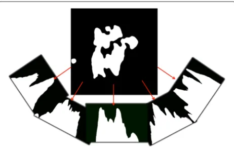
Figure 11-D projections are taken of a 2-D object.The small ball along the edge is not projected in the 0° projection straight down due to the limited projection range. However, at the higher angles, this mass is now projected, which will affect an alignment based on the center of mass of these projections.

Fiducial marker tracking is done by decorating the sam-ple with small high-density particles that create high con-trast in the projection images [9-12]. Individual markers are then identified in all projections. The alignment is determined based on tracking of the path of each marker through the projections. This method can be very accu-rate but requires a lot of manual interaction to properly locate and center the markers. The main drawback of marker tracking is that the markers will be present in the reconstruction and must be removed for accurate characterization of the sample. Since the markers are of such high density, the reconstruction of the markers will inevitably mix with the reconstruction, making the task of removal nontrivial and possibly inaccurate.

Feature tracking uses regions of high contrast or inten-sity as fiducial markers [13,14]. It requires the identifica-tion of suitable regions of high contrast that remain visible throughout the tilt series.

Others have begun to perform alignment techniques based on a refinement approach [6]. After a coarse align-ment from cross-correlation, one proceeds in computing an initial 3-D reconstruction. This 3-D reconstruction is then reprojected and compared with the original projec-tions. A new alignment arises from aligning the repro-jected reconstruction with the original projections, and this process is iterated until convergence is met. In our experience with this method, the reconstruction always satisfies the projections, even if they’re misaligned, so that insignificant refinement occurs from updating.

Most recently, Scott et al. [15] introduced a technique based on the observation that as the sample is tilted about a fixed axis, the center of mass of the sample will spin in a circle, and if the center of mass is on the tilt axis, then it remains fixed. In this way, it was suggested to shift each projection so that the center of mass in each projection is

fixed on a point and taking the line through this point par-allel to the axis of rotation as the tilt axis. We believe this is not always applicable and can yield poor results in many settings. First, it requires a tilt series in which the total projected volume is fixed for each projection. However, in most practical settings, some mass will move in and out of the projection range as the sample is tilted, which will then significantly affect the location of the center of mass within the projection along both axes of the projec-tion images. This transiprojec-tion of mass must be accounted for, as this transition will be along the edges of the projec-tions, far from the center, and will thus weigh heavily on the calculated center of mass. Figure 1 demonstrates this transition of mass, with the small ball located on the left edge of the object that has only been projected at certain angles. An additional drawback is that using only the sin-gle center of mass point in each projection removes the use of any local structure of the projections as criteria for alignment.

In this paper, we give an alignment method that makes more detailed use of the path of the projected center of mass along many cross-sections of the object, perpendic-ular to the axis of rotation. In an ideal experiment, points on the sample move in circular trajectories. We define a viable path as the projection of such a circular orbit. By simple calculation, we derive an equation which describes all such viable paths of the projected centers of mass, as opposed to the one trivial path of a single point. From here, we show how one can determine a shift for each projection so that the center of mass of all cross-sections perpendicular to the axis of rotation nearly follows a viable path. In this way, since all cross-sections are considered in our alignment method, we will be able to avoid problems involved with error in the calculated centers of mass due to transition of volume in and out of the projections, and we maintain local analysis of the projections as means for the alignment. Additionally, our model aligns the projec-tions based on the rotation about a chosen axis, so that manual interaction for determining the positioning of the tilt axis is avoided. In general, our method can be con-sidered more statistically accurate, and we will show that it provides very dependable alignment and definitively improves the resolution of the reconstruction.

Methods Notation

The 3-D density function for reconstruction will be denotedf(x,y,z)=f(x,(y z)), with(y z)a 2-D row vector. The data generated are the projections off in thez-axis, about rotations around thex-axis. A rotation off through

θ about thex-axis can be written as:

f(x,(y z)Qθ), where Qθ =

cosθ −sinθ sinθ cosθ

A projection about the rotationθ is then defined as:

Pθ(f)(x,y)=

Rf(x,(y z)Qθ)dz.

We note that for each fixed x = x0, Pθ(f)(x0,y) only

contains information fromf(x0,y,z), and therefore, many

of the alignment and reconstruction processes can be considered as 2-D rather than 3-D. Therefore, for conve-nience, we will sometimes denote:

fx(y,z)=f(x,y,z) and Pθ(fx)(y)=Pθ(f)(x,y).

In practice, we are given the unaligned data; there-fore, we will regularly refer to the misaligned projections, denoted byPθ(f). We define these projections as:

Pθ(f)(x,y)=Pθ(f)(x−xθ,y−yθ),

where the coordinates(xθ,yθ)are the shifts to be deter-mined for the alignment. Similarly, we will denote:

Pθ(fx)(y)=Pθ(fx)(y−yθ),

where in this instance the shift xθ is not included. We do not include it, for determining the shiftsxθ is a much more trivial task, so that most of our work here focuses on determiningyθafter thex-axis alignment is completed.

We will denote the total mass about a cross-sectionx byMx =

R2fx(y,z)dy dz. Then, the coordinates for the center of mass of a cross-section are denoted as:

cyx= 1 Mx

R2fx(y,z)y dy dz, c z x=

1 Mx

R2fx(y,z)z dy dz We will denote the center of mass of a projected cross-section off by:

tθ_x= 1 Mx

RPθ(fx)(y)y dy, and ˜t θ

x= 1 Mx

RPθ(fx)(y)y dy We take the conventionalLpnorm (denoted by · p) of a function, sayg, defined overRn_{to be:}

gpp=

Rn|g(x)|

p_dx.

Similarly, for a vector x ∈ Rn, we take the p norm (denoted · p) to be:

xpp= n

i=1

|xi|p.

Theoretical model

In practice, we are given the set of misaligned angular projections:

P_θi(f)(x,y), for i=1, 2,. . .,k.

Typically, the number of projections, k, can be from 50 to 200, with maximum tilts of± 70°. The domain is of course limited, but for theoretical purposes, we will assume that the domain for y is all of R. The prob-lem is then to approximate the set of shifts (xθi,yθi) for alignment, so that Pθi(f)(x,y) k_i=1 correspond to the aligned projectionsPθi(f)(x,y) k_i=1. Determining the shifts for the x-axis is much simpler, since the x-axis is the axis of rotation. We simply observe that the total mass in each cross-section should remain fixed, so that:

Mx=

R2fx(y,z)dy dz=

RPθi(fx)(y)dy. (1)

Based on this simple observation, one should be able to approximate all shiftsx_θi based on a ‘conservation of mass’ approach. We design a ‘global’ alignment method for determining these shifts, by takingxθito be the shift which minimizes the difference between the observed mass in each cross-section ofPθi(f)(x−xθi,y)and the average mass of all projections in each cross-section. More precisely, we let:

x_θi=arg min

x∗

RPθi(f)(x−x

∗_,y)dy−1

k

k

l=1

RPθl(f)(x,y)dy

₁. (2)

Of course, the averaged term, 1_kk_l=1RPθl

(f)(x,y)dy, is subject to error since the projections are not yet aligned, so the determination of each xθi is iterated a few times until there is no change. The number of iterations will depend on just how large the offset of the projections are, but we have typically observed no change in eachx_θi after just two iterations. A demonstration of this x-axis alignment is given in Figure 2.

One could also perform a similar ‘local’ method, by comparing the consecutive projections to each other instead of the average. This approach is subject to cumu-lative error in the alignment similar to cross-correlation; therefore, we avoid this approach.

From here forth, we will now assume that thex_θi have been accurately determined, and consider each cross-section. For alignment along the y-axis, we again want to make use of physical properties. It has been noted, asfx(y,z)is rotated about the origin, the center of mass

cyx,czx

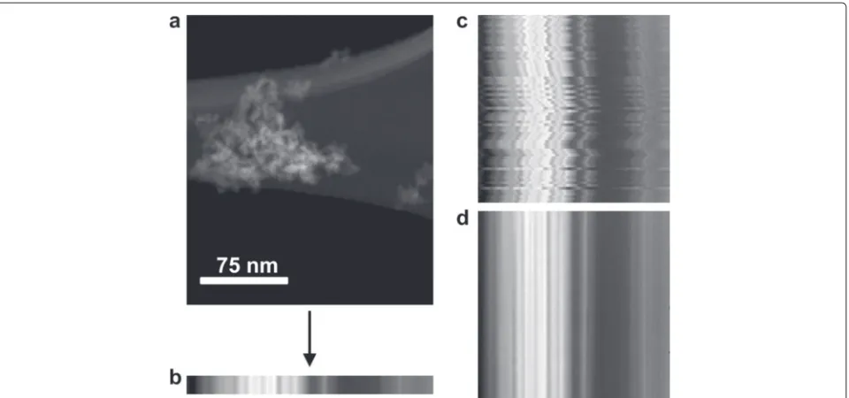
Figure 2Images demonstrating the alignment along thex-axis.(a)2-D projection image taken at a 30°tilt about thex-axis.(b)1-D projection of (a)onto thex-axis.(c)1-D projections onto thex-axis of all 2-D projections taken at different tilts about thex-axis. The misalignment is clearly shown in(c), as the 1-D projections should all be nearly the same.(d)Same 1-D projections in(c), shown after alignment is performed along thex-axis.

tθi x =

1 Mx

RPθi(fx)(y)y dy

= 1

Mx

R

Rfx((y z)Qθi)y dz dy = 1 Mx R

Rfx(α,β)(αcosθi−βsinθi)dαdβ

=cos_Mθi x

R

Rfx(α,β)αdαdβ−

sinθi

Mx

R

Rfx(α,β)βdαdβ

=cyxcosθi−czxsinθi,

where we applied the substitution(α β):=(y z)Qθi. This tells us that the center of mass of each projected cross-section should follow the path given by:

t_xθi=cyxcosθi−cxzsinθi, for i=1, 2,. . .,k. (3) This equation gives us a local relationship between the relative positioning of all of the projections to use for the alignment. As discussed earlier, in [15], it was simply noted that if the center of mass is located at the origin on the tilt axis, then it does not move under rotations about that axis. This observation can be made through similar computations where the integrand is first taken over x, and then, the center of mass is computed for the total sum of the cross-sections, that is:

tθi= 1 M

R2

P_θi(f)(x,y)dx y dy=cycosθi−czsinθi,

(4)

where cy andcz here denote the center-of-mass coordi-nates along they- and z-axes, respectively, independent ofx, andMdenotes the total mass off. Therefore, it is

suggested to shift each projection so thattθi =0 for alli, so thatcy = cz = 0. While this approach is theoretically sound in an ideal setting, summing over ximmediately removes any consideration of local behavior of the pro-jections of f. As we will show, in many settings, this simplification can be a major drawback.

Therefore, our approach is to determine a sequence of shifts so that for each cross-section there exists some deterministic center of masscyx,czx

so that Equation 3 is nearly satisfied. With this in mind, let us denote:

= ⎛ ⎜ ⎜ ⎜ ⎝

cosθ1−sinθ1

cosθ2−sinθ2

..

. ...

cosθk−sinθk

⎞ ⎟ ⎟ ⎟ ⎠, cx=

cyx cz_x

, and tx=

⎛ ⎜ ⎜ ⎜ ⎜ ⎝ ˜ tθ1

x ˜ tθ2

x .. . ˜ tθk

x ⎞ ⎟ ⎟ ⎟ ⎟ ⎠.

We note that from the acquired projection data we can compute bothandtx. Now from Equation 3, if our align-ment is good, then for each cross-sectionx, there should exist somecxso thatcx ≈tx. Therefore, in order to yield a good alignment, we would like to determine:

y=

⎛ ⎜ ⎜ ⎜ ⎝

yθ1 yθ2 .. . yθk ⎞ ⎟ ⎟ ⎟ ⎠,

so that there exist somecxsatisfying:

min

cx cx−(tx+y)

2

2≈0 for allx.

In practice, we will have some finite number of cross-sections, say xj, for j = 1, 2,. . .n. Then, we would like solve the minimization problem:

min y

⎛ ⎝n

j=1

min

c_xj cxj−(txj+y)

2 2

⎞

⎠ (5)

Now we can compute the minimization overcxdirectly. Givenandtx, the least square solutionc∗x, tocx−(tx+ y)22 :

c∗_x =arg min

cx cx−(tx+y)

2 2,

can simply be found by differentiation so that:

_∂

∂cyx

cx−(tx+y)22 cx=c∗x =0 and

∂

∂czx

cx−(tx+y)22

cx=c∗x =0.

Solving these equations, the solution can be found to be:

+(tx+y),

where + denotes the pseudo-inverse of , given by

+₌₍T₎−1_{. It should be noted that}T_{is a 2×2} matrix with entries:

(T₎

11=

k

i=1

cos2θi, (T)21=(T)12

= −

k

i=1

cosθisinθi, (T)22=

sin2θi, which is clearly invertible and without any notable com-putational cost.

Then, our minimization in Equation 5 becomes:

min y

⎛ ⎝n

j=1

+(txj+y)−(txj+y)

2 2 ⎞ ⎠ =min y ⎛ ⎝n

j=1

(+−I)(txj +y)22

⎞

⎠. (6)

If we let:

A= ⎛ ⎜ ⎜ ⎜ ⎝

+_−I

+_−I

.. .

+_−I

⎞ ⎟ ⎟ ⎟

⎠, and b= ⎛ ⎜ ⎜ ⎜ ⎝

(+_−I)t

x1

(+_−I)t

x2 .. .

(+_−I)t

xn ⎞ ⎟ ⎟ ⎟ ⎠,

then the minimization problem in Equation 6 is equivalent to solving a standard least squares problem:

min

y Ay−b

2

2. (7)

Practical implementation

The major consideration that we have ignored so far in the theoretical development but will handle in this section is that certainly the domain for yforP_θi(fx)(y) is finite, say [−m,m]. As before withx, for all practical purposes, we will now additionally consider the y-axis to be dis-crete, and for each projectionPθi(f)(x,y), the domain is given as:

D= {(x,y): x=1, 2,. . .,n, y= −m,−m+1,. . .,m}.

We chose the indexing for ysymmetrically for conve-nience in the center-of-mass computations so that the center of the projections is along the modeled axis of rotation aty=0. Computingtθix now becomes:

t_xθi= 1 Mx

m

y=−m

Pθi(x,y)y.

The first issue is thatMxmay vary through the tilt series for each cross-section; in particular, since the domain for yis limited, there may be some observable mass moving in and out of the field of view after rotation and projec-tion, as we demonstrated in Figure 1. This is again why it’s important that we choose the alignment to be considered over many projected cross-sections.

To handle this issue, we multiplyP_θi(f)(x,y)by a win-dow function,ω_θi(x,y), in the computation oftθix in order to alleviate some of this transition of mass in and out of the frame. The window function allows for the balance of the total mass within each projection. We choose our window functions to satisfy the following properties:

(i) 0≤ωθi(x,y)≤1;

(ii) M=n_x=1m_y=−mPθi(f)(x,y)ωθi(x,y), for i=1, 2,. . .,k;

(iii) ωθi(x,y)≤ωθi(x,y+1) if y<0,

ωθi(x,y)≥ωθi(x,y+1) if y≥0;

(iiii) ωθi(x,y)=ωθi(x+1,y), forx=1, 2,. . .,n−1.

cross-section of each projection. This could potentially cause bias in the alignment of the cross-sections, espe-cially ones with considerable noise, and it would require much greater computational time to determine a window for each cross-section of each projection.

After the windowing function is determined, we then compute the center of mass for each projected cross-sectiontxj, forj=1, 2,. . .,nas:

˜ t_xθi_j = 1

Mxθij

m

y=−m

P_θi(fxj)(y)ωθi(y)y and txj =

⎛ ⎜ ⎜ ⎜ ⎜ ⎝ ˜ tθ1

xj ˜ tθ2

xj .. . ˜ txθkj

⎞ ⎟ ⎟ ⎟ ⎟ ⎠,

and solve a variant of Equation 6. The variation is that we only choose to minimize only a subset of the cross-sections, say T ⊂ {1, 2,. . .,n}. This subset is chosen so that the selected cross-sections have a significant quan-tity of mass in each projection so that introduction of new mass along the edges has considerably less effect on the center of mass of this projected cross-section area. In addition, we only choose those in which the observable total mass within that cross-section varies little through-out all projections, to again avoid the cross-sections with large transition of mass.

More precisely, we pick the cross-sections in which the ratio of the average observed mass through the projec-tions to the variance of the mass in the projecprojec-tions is above some specified tolerance. This tolerance can be chosen based upon quality of the data. Finally, the minimization for determining the shifts becomes:

min y

⎛

⎝

j∈T

(+−I)(y+txj)22

⎞

⎠, (8)

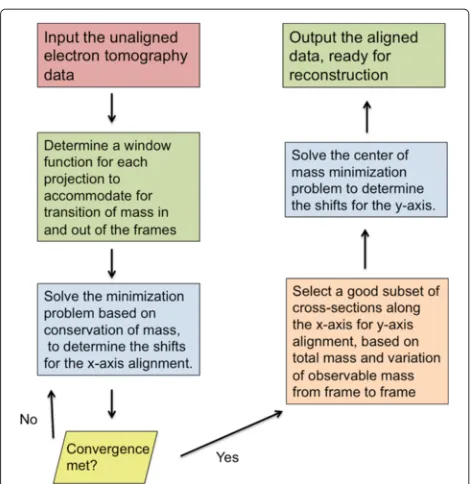
which can again be converted into a standard least squares minimization problem as done in Equation 7. We sum-marize the method with the simple schematic shown in Figure 3.

Reconstruction method

After the alignment, for the reconstruction, we use a compressed sensing approach by total variation (TV) min-imization [16]. These methods have recently been gain-ing popularity for electron tomographic reconstructions [17-19]. In order to briefly describe the method, let us denote the 3-D reconstructed approximation off byg = {gx,y,z}N_x,y,z=1, where for simplicity we now let our discrete 3-D domain be:

D=(x,y,z):x,y,z∈ {1, 2,. . .,N} .

Most reconstruction methods are then designed so that numerical reprojection of g agrees with the experimen-tal projections Pθi(f), for i = 1, 2,. . .,k. In particular,

Figure 3The general workflow of our alignment approach.

reconstruction techniques typically minimize the distance between the projections ofgand the experimental tions, sometimes called the projection error. This projec-tion error can be expressed as:

k

i=1

dist(Pθi(f),Pθi(g))

2₌

k

i=1

N

x,y=1

Pθi(f)(x,y)−Pθi(g)(x,y) 2

.

(9)

However, simple minimization of the projection error does not necessarily produce optimal results in the pres-ence of noise. Therefore, methods, such as TV minimiza-tion, additionally apply regularization conditions on the reconstruction. In the case that our sample consists of homogeneous materials and relatively smooth surfaces, compressive-sensing theory allows us to assume that the reconstruction should have a small total variation norm, given by:

gTV= N

x,y=1

N−1

z=1

|gx,y,z+1−gx,y,z|+ N

x,z=1

N−1

y=1

|gx,y+1,z−gx,y,z|

+

N

y,z=1

N−1

x=1

|gx+1,y,z−gx,y,z|.

With this in mind, we would like for Equation 9 to be relatively small, while also applying a penalty ongTVfor noise reduction, so that our method solves:

min g

gTV+λ k

i=1

Results and discussion

We will give the results for experimental and simulation data. We compare the reconstructions from alignment using cross-correlation and our center-of-mass technique, while also demonstrating the advantage of using many slices for the center-of-mass alignment, as opposed to just one center-of-mass calculation.

Experimental results

For the experimental data, we have an alumina particle sitting on a holey carbon grid. The sample was prepared by grinding the alumina spheres into powder. A suspen-sion of the powder is prepared in ethanol and sonicated for 5 min. The suspension was then added drop-wise over

the lacey carbon film supported on 200 mesh Cu TEM grids (Structure Probe, Inc., West Chester, PA, USA) and dried at room temperature. The sample is analyzed using the FEI Titan 80-300 Scanning Transmission Electron Microscope equipped with a spherical-aberration probe-corrector (CEOS GmbH, Heidelberg, Germany) operating at 200 kV. The images were collected using the high-angle annular detector with the camera length of 195 mm and at 80,000Xmagnification. The acquisition time was set to 15 s over an image area of 1024X1024 pixels resulting in a pixel size of 0.2411 nm. The tilt series is collected using linear tilt scheme continuously from -70° to +70°with tilt increments of 2°. Dynamic STEM focus function is used to compensate for change in focus across the image.

The projection of the sample at 30°degrees is shown in Figure 2, and the aligned projections are shown in a video in Additional file 1.

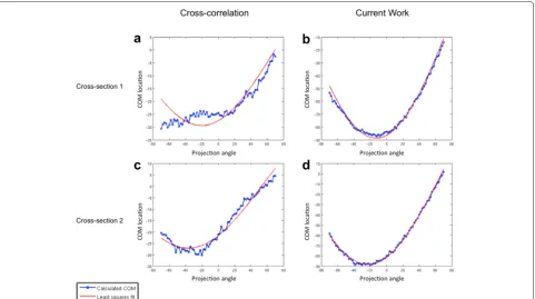
Total variation minimization is valid for this data set, as the alumina particle and the carbon grid are known to be uniform in density. In addition, regularization of the reconstruction with TV minimization is critical to the quality of the results due to the low-dose sampling con-ditions necessary for acquisition of the projections due to beam sensitivity of the material. The reconstructed images from cross-correlation and our alignment meth-ods are shown in Figure 4. While the overall particle morphologies are similar, the reconstruction resulting from our alignment displays much more uniform den-sities and clearer particle structures. This will result in more confident segmentation and characterization of the reconstructed particle, which is crucial to the interpre-tations of the experiment. In the 3-D images (visualized using tomviz software [20]), the overall structures appear similar. However, less rigid particle structure is recov-ered with the cross-correlation alignment, as the red glow around the particle demonstrates blurring from the main particle structure to a lower gray level represented by red in the colormap. In Figure 5, we plotted the cen-ters of mass, tx, for two cross-sections. Plotted together

withtx are least squares solutions of the center of mass,

(cyx,czx), based Equation 3 given the computed tx. It is evident that our method finds a nearly viable path for the motion of the center of mass, as we set out to do. On the other hand, the alignment from cross-correlation clearly fails to do so, resulting in low-resolution reconstructions.

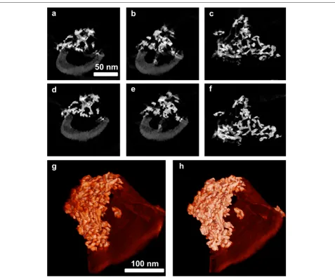
In Figure 6, additional results are given using the align-ment method described in [15]. Again the 3-D visual comparison of the reconstructions show that our align-ment has produced a more rigid structure, as there is less red glow from the main particle but less significant than the results from cross-correlation. Similarly, the images in Figure 6c,d,e,f of the 2-D cross-sections show a more rigid structure and less noisy artifacts due to misalign-ment. The plots in Figure 6 give a quantitative comparison of the alignment approaches. In Figure 6g,h, the location of the global projected center of mass along they-axis is shown for the two methods. The plot in Figure 6g shows the only consideration for the originally proposed center-of-mass alignment, as the center of mass in the projections along the y-axis is shifted to the tilt axis. With pixela-tion of the images, there is still a small negligible distance (less than half a pixel) between the center of mass in each projection and the tilt axis. The location of this center of

Figure 6Results from alignment in [15] and our approach.(a, b)Images of 3-D volume rendering of the reconstructions from the [15](a)and our method(b).(c, e)2-D cross-sections images of the 3-D reconstruction shown in(a).(d, f)Images of corresponding 2-D cross-sections of the 3-D reconstruction shown in(b).(g, h)Plots of the path of the projected global center of mass along they-axis for the two alignment methods.(i, j) Plots of the path of a center of mass along a single cross-section of the projections for the two alignment methods.

mass resulting from our approach is shown in Figure 6h and does not necessarily follow a viable path, because we choose a different minimization and allow our approach to avoid problematic cross-sections. In Figure 6i,j, the path of the projected center of mass is shown for a sin-gle cross-section for the two alignment methods, where, for this cross-section, our methods demonstrate a viable path and the approach based on the single global cen-ter of mass does not. Inevitably, our method produces better reconstruction results, demonstrating that a more sophisticated alignment approach should be taken for dependable results as we have done, taking into account not one single data point but rather all cross-sections as unique data points. The resulting segmentation of the alu-mina particle is shown in 3-D in a video in the Additional file 2.

Simulation results

Figure 7Tomographic simulations with a binary 3-D phantom.(a, b)Projection images of the phantom tilted about the axis at -50° and -32°, respectively.(c-e)2-D cross-section of the reconstructed phantom from registering the data with different alignment techniques.(c)Result from our center of alignment method.(d)Result from cross-correlation.(e)Result from originally proposed center-of-mass technique.

range. With the special example we have here, this small transition of mass will significantly affect the results of an alignment approach such as in [15]. This is very clear from the resulting blurry reconstruction in Figure 7e that does not resemble a binary reconstruction. In addition, it can be seen in Figure 7d that even in this noise-free simulation cross-correlation also produces very poor results simply because the model is not appropriate. In Figure 7c, it is seen that our center-of-mass approach still yields optimal results displaying a near binary reconstruction image that almost completely resembles the original phantom not presented in the figure. The adaptability of our method to choose only the appropriate cross-sections with little vari-ability of mass is clearly advantageous as demonstrated in these simulations.

Conclusions

Our method has a sound physical basis: the movement of the center of mass in each cross-section. By select-ing shifts for individual tilt-series images that globally lead to physically plausible motions for the centers of mass of many cross-sections, our method effectively uti-lizes the assumption that the sample object is rigid to improve the alignment and the resolution of the final reconstruction. We have shown that conventional align-ment procedures, which shift the global center of mass to the origin, may not produce physically plausible motions in other cross-sections. We have generalized these meth-ods in a computationally feasible manner that can be easily be incorporated into electron tomography work-flows. We have demonstrated the significance of such

consistency between cross-sections and the effective-ness of the presented method by improving the reso-lution of 3-D reconstructions of simulated and actual data.

Additional files

Additional file 1: Video that shows the sequence of aligned projection images of the alumina particle using the method proposed in this paper.

Additional file 2: Video that shows the reconstructed alumina particle in 3-D.

Competing interests

The authors declare that they have no competing interests.

Authors’ contributions

TS derived the alignment methods and algorithms. TS and MP analyzed the technical issues of the methods and algorithms. PB assisted in the analysis of the methods and supervised the research. CA generated the tomography data and analyzed the quality of the reconstructions. TS created the simulated tomography data. TS performed the alignment and reconstruction algorithms and performed the analysis. TS drafted the manuscript. TS and MP revised the manuscript, and all authors discussed it. All authors read and approved the final manuscript.

Acknowledgements

The authors would like to thank Dr. Ilke Arslan for her helpful discussions. This research was supported in part by NSF grant DMS 1222390. It was also funded by the Laboratory Directed Research and Development program at Pacific Northwest National Laboratory, under contract DE-AC05-76RL01830.

Author details

1_{Department of Mathematics, University of South Carolina, 1523 Greene}

Received: 25 November 2014 Accepted: 13 February 2015

References

1. Lucic, V, Forster, F, Baumeister, W: Structural studies by electron tomography: from cells to molecules. Ann. Rev. Biochem.74, 833–865 (2005)

2. Midgley, P, Weyland, M: 3D electron microscopy in the physical sciences: the development of Z-contrast and EFTEM tomography. Ultramicroscopy. 96, 413–431 (2003). International Workshop on Strategies and Advances in Atomic-Level Spectroscopy and Analysis (SALSA), GUADELOUPE, GUADELOUPE, MAY 05-09, 2002

3. Arslan, I, Yates, T, Browning, N, Midgley, P: Embedded nanostructures revealed in three dimensions. Science.309(5744), 2195–2198 (2005) 4. Crowther, RA, Amos, LA, Finch, JT, De Rosier, DJ, Klug, A: Three

dimensional reconstructions of spherical viruses by Fourier synthesis from electron micrographs. Nature.226(5244), 421–425 (1970)

5. Arslan, I, Tong, JR, Midgley, PA: Reducing the missing wedge: high-resolution dual axis tomography of inorganic materials. Ultramicroscopy. 106(11–12), 994–1000 (2006). Proceedings of the International Workshop on Enhanced Data Generated by Electrons Proceedings of the International Workshop on Enhanced Data Generated by Electrons. 6. Houben, L, Sadan, MB: Refinement procedure for the image alignment in

high-resolution electron tomography. Ultramicroscopy.111(9–10), 1512–1520 (2011)

7. Guckenberger, R: Determination of a common origin in the micrographs of tilt series in three-dimensional electron microscopy. Ultramicroscopy. 9(1–2), 167–173 (1982)

8. Saxton, W, Baumeister, W, Hahn, M: Three-dimensional reconstruction of imperfect two-dimensional crystals. Ultramicroscopy.13(1–2), 57–70 (1984)

9. Brandt, S, Heikkonen, J, Engelhardt, P: Multiphase method for automatic alignment of transmission electron microscope images using markers. J. Struct. Biol.133(1), 10–22 (2001)

10. Fung, JC, Liu, W, de Ruijter, W, Chen, H, Abbey, CK, Sedat, JW, Agard, DA: Toward fully automated high-resolution electron tomography. J. Struct. Biol.116(1), 181–189 (1996)

11. Masich, S, Östberg, T, Norlén, L, Shupliakov, O, Daneholt, B: A procedure to deposit fiducial markers on vitreous cryo-sections for cellular

tomography. J. Struct. Biol.156(3), 461–468 (2006)

12. Ress, D, Harlow, M, Schwarz, M, Marshall, R, McMahan, U: Automatic acquisition of fiducial markers and alignment of images in tilt series for electron tomography. J. Electron Microsc.48(3), 277–287 (1999)

year=1999,

13. Brandt, S, Heikkonen, J, Engelhardt, P: Automatic alignment of transmission electron microscope tilt series without fiducial markers. J. Struct. Biol.136(3), 201–213 (2001)

14. Sanchez Sorzano, CO, Messaoudi, C, Eibauer, M, Bilbao-Castro, JR, Hegerl, R, Nickell, S, Marco, S, Carazo, JM: Marker-free image registration of electron tomography tilt-series. BMC Bioinformatics.10, 124 (2009). http://biocomp.cnb.csic.es/~coss/Articulos/Sorzano2009b.pdf 15. Scott, MC, Chen, C-C, Mecklenburg, M, Zhu, C, Xu, R, Ercius, P, Dahmen, U,

Regan, BC, Miao, J: Electron tomography at 2.4-angstrom resolution. Nature.483(7390), 444–U91 (2012)

16. Li, C: Compressive sensing for 3D data processing tasksapplications, models, and algorithms. Dissertation, Rice University (2011)

17. Leary, R, Saghi, Z, Midgley, PA, Holland, DJ: Compressed sensing electron tomography. Ultramicroscopy.131, 70–91 (2013)

18. Goris, B, den Broek, WV, Batenburg, K, Mezerji, HH, Bals, S: Electron tomography based on a total variation minimization reconstruction technique. Ultramicroscopy.113, 120–130 (2012)

19. Monsegue, N, Jin, X, Echigo, T, Wang, G, Murayama, M: Three-dimensional characterization of iron oxide (alpha-Fe2O3) nanoparticles: application of a compressed sensing inspired reconstruction algorithm to electron tomography. Microscopy Microanal.18(6), 1362–1367 (2012) 20. Tomviz for tomographic visualization of 3D scientific data. http://www.

tomviz.org (2014). 15 August 2014.

Submit your manuscript to a

journal and benefi t from:

7Convenient online submission 7Rigorous peer review

7Immediate publication on acceptance 7Open access: articles freely available online 7High visibility within the fi eld

7Retaining the copyright to your article