Portfolio theory for squared returns correlated across time

and Quantitative Risk

R E S E A R C H Open Access

Portfolio theory for squared returns correlated

across time

Ernst Eberlein · Dilip B. Madan

Received: 12 January 2016 / Accepted: 10 June 2016 /

© The Author(s). 2016Open AccessThis article is distributed under the terms of the Creative Commons Attribution 4.0 International License (http://creativecommons.org/licenses/by/4.0/), which permits unrestricted use, distribution, and reproduction in any medium, provided you give appropriate credit to the original author(s) and the source, provide a link to the Creative Commons license, and indicate if changes were made.

Abstract Allowing for correlated squared returns across two consecutive periods, portfolio theory for two periods is developed. This correlation makes it necessary to work with non-Gaussian models. The two-period conic portfolio problem is formu-lated and implemented. This development leads to a mean ask price frontier, where the latter employs concave distortions. The modeling permits access to skewness via randomized drifts. Optimal portfolios maximize a conservative market value seen as a bid price for the portfolio. On the mean ask price frontier we observe a tradeoff between the deterministic and random drifts and the volatility costs of increasing the deterministic drift. From a historical perspective, we also implement a mean-variance analysis. The resulting mean-variance frontier is three-dimensional expressing the minimal variance as a function of the targeted levels for the deterministic and random drift.

Introduction

A persistent empirical observation about equity market returns is that even though they tend to be uncorrelated across two successive time periods, they are not indepen-dent, as the squared returns are highly correlated (see for example Barndorff-Nielsen and Shepard (2002) and the references cited therein) with correlation coefficients as high as seventy percent. A natural question, arising as a consequence of such intertemporal correlations, are the portfolio theoretic implications of such facts. In particular, we ask how allocations move between time periods when correlations rise

E. Eberlein ()

University of Freiburg, Freiburg im Breisgau, Germany e-mail: eberlein@stochastik.uni-freiburg.de

D.B. Madan

and do the results also dependent on other underlying market conditions. To answer such questions we consider a three date, two-period model for investment opportu-nities permitting correlation in squared returns between the periods. More dynamic models including continuous-time models could also be developed (see for example Basak and Chabakauri (2010)), but the simpler two-period model serves as a useful building block. In this regard, we build upon the single-period fundamental portfolio theory of Markowitz (1952, 1991).

For a two-period model it is natural to take the investment criterion as applying to the aggregate two-period return. Since much has been written on the portfolio the-ory for a single investment period from a mean-variance perspective, we include an analysis of the two-period problem from a similar perspective. A number of authors have considered a multi-period mean-variance formulation (see for example, among others, Acharya and Pedersen (2005), Ait-Sahalia and Brandt (2001), Bansal, et al. (2004), Brandt (2009) Campbell and Viceira (2002), Hong, et al. (2006), Jagannathan and Ma (2003)), but from the myopic perspective of optimizing the one-step ahead objective function. However, we also recognize some of the shortcomings of mean-variance theory with its use of rewards being measured in units that do not tally with those used for risk. Furthermore, the criterion is not arbitrage consistent as a posi-tive cash flow accessed at zero cost is desirable whatever its variance. We are thus led to primarily consider alternative criteria. To limit the analysis we select a single alternative.

The possibilities include expected utility theory, other risk measures like semivari-ance, value at risk, or the expected shortfall. Expected utility theory does not focus attention on the allocation problem as it seeks to determine the actual size of posi-tions. It is also difficult to accommodate losses with a dimensionless risk aversion coefficient. Some of the other risk measures may be related to special cases of the recently proposed conic portfolio theory objectives proposed in Madan (2016). The criterion of conic portfolio theory is to maximize a conservative future market value viewed as the infimum of valuations taken with respect to a number of candidate test probabilities. The result can be written as the mean less the supremum over a set of probabilities of the expectation for the negative of the centered return. The latter may be seen as a positive market ask price and serves as the embedded risk measure. Being positive, it is bounded below by zero and leads to a natural mean ask price efficiency frontier. The conservative value maximizing portfolio is then located on this frontier at a point where the slope of the frontier is unity. This is because the conservative value is just the difference between the mean and the ask price so the rate of exchange between the mean and the ask price is always unity. Greater risk aversion is accom-modated by expanding the set of probabilities with respect to which one takes the infimum in defining the conservative value or, equivalently, the supremum in defin-ing the ask price. We present an analysis of the two-period portfolio problem from the perspective of conic portfolio theory applied to the aggregate two-period return.

We build as information for the investment decision the joint law for the returns over two periods, where the law is known and has been estimated at the start of the first period. In particular, there isn’t a Markovian structure with the distribution of second-period returns responding to actual realizations in the first second-period. The realizations are seen as quite noisy with little or no impact on the prior estimated distribution for the second period. We recognize that if there was a firmly asserted joint law, then one could be Bayesian and attempt to infer the conditional second-period law to be used for the second-period decision. Such a procedure places considerable faith in the asserted two-period law and our criterion is going to take the infimum over many test probabilities as none of them are believed to be relevant with enough confidence to be used in a Bayesian construction. We therefore commit to second-period invest-ments at the start of the first period and then evaluate the aggregate portfolio return at the end of two periods.

There is an extensive literature applying such precommitment investment policies. We may cite as examples Bajeux-Besnainou and Portait (1998), Bielecki et al. (2005), Cvitanic et al. (2008), Cvitanic and Zapatero (2004), MacLean et al. (2011) and Cochrane (2014). Such precommitment solutions are also obtained in Duffie and Richardson (1991) in a continuous-time incomplete markets setting while Leippold et al. (2004) work in a discrete-time complete markets setting, whereas, Zhou and Li (2000), and Lim and Zhou (2002) approach the problem in a continuous-time complete markets setting. Basak and Chakabauri (2010) are critical of such precom-mitment policies arguing that they are not likely to be time consistent and leave incentives open for investors to deviate from the precommitment positions. They argue, in line with Strotz (1956), that rational decision making should be time con-sistent involving plans that will in fact be followed. However, this is time consistency within a model of information evolution that rational decision makers recognize, will be called into question. The incentive to deviate then remains for time consistent solu-tions as and when the information evolution models are questioned, reformulated or re-estimated. Such super-rationality is not possible for long and at best we may hope to precommit for a short period. The reasons for deviation are many and we focus attention here on just a two-period precommitment.

We recognize that, classically, portfolio problems are analysed in the context of the presence and absence of a risk-free asset. We therefore develop both approaches over two periods from both a conic and mean-variance perspective. However, if the holding period is not locked in, then fixed income securities are exposed to the risk of movements in interest rates and their return is no longer risk free. Many fixed-income investments are spread over multiple maturities with exposure to interest rate risk making them no longer risk-free and then also correlated with equity returns. The more reasonable and economically relevant perspective is then that for the absence of a risk-free asset. In fact, on recognizing that a credit default swap trades on the debt of the US Treasury leads one to conclude that the US Treasury cannot credibly promise a future dollar. In which case no one can. A risk-free asset is then a fiction that perhaps has outlived its usefulness.

portfolio optimization problem is numerically tractable. We also reduce the two-period mean-variance problem to a fixed point problem that is numerically solved.

The outline of the rest of the paper is as follows. Section “Two-period return mod-eling” takes up the two-period conic portfolio theory and the associated mean ask price frontier. Section “Two-period portfolio theory from a conic perspective” also presents the details for the construction of investment opportunity frontiers for conic portfolio theory allowing access to both correlated squared returns across time peri-ods and access to random drifts that leverage the design of skewness in portfolio construction. Section “Conservative value maximizing portfolios across two-periods with correlated squared returns” takes up the implementation of two-period conic portfolio theory. Section “Two-period mean-variance analysis” presents an analysis of the problem from the mean-variance perspective developing the two-period port-folio theory along with the two-period mean-variance frontier and the procedures for its computation. Section “Conclusion” concludes. All proofs are provided in the Appendix.

Two-period return modeling

Consider the context of an initial wealthV0invested innrisky assets. Let the

first-and second-period risky asset returns be given by rfirst-andomn-dimensional vectors of

R1, R2,respectively. If the time zero and time one dollar investments in thenassets

are given by n-dimensional vectors a0, a1, respectively, then the random wealth

accumulated at the end of the second period is

V2=V01+a₀R1 1+a₁R2.

With a view towards accomodating correlation in squared returns we model returns on the basis of time changed L´evy processes where we correlate the subordinators which are used for the time changes. We therefore write

R1 = X1(T1)+μ1 (1)

R2 = X2(T2)+μ2, (2)

whereX1(t), X2(t)are zero-mean multivariate L´evy processes which are assumed to

be independent of each other and independent of the time changesT1andT2.1, 2

denote the covariance matrices ofX1(1), X2(1). In case these variables are

one-dimensional, we shall writeσ₁2, σ₂2for their variances. To accomodate correlation in

squared returns we modelT1, T2as

T1 = G(α1)+G1(1−α1) (3)

T2 = G(α2)+G2(1−α2), (4)

for subordinatorsG, G1, G2and 0≤α1, α2≤1.These three processes are assumed

to be independent and also independent of X1, X2. For reasons of tractability of

with unit mean rate and variance rateν, ν1, ν2,respectively. To be more precise, the

characteristic function ofG(1)is

Eexp(iuG(1))=

₁

1−iuν 1

ν

.

In the special case ofν1=ν2=ν,it is easy to see that the random timesT1, T2

are themselves gamma distributed with unit mean and varianceν.

When the processesXi(t)being time changed are Brownian motion with driftθ ,

the resulting asset returns have a variance gamma distribution. Let us look at this particular specification from an empirical point of view. For this purpose, introduce two random variablesZ1, Z2as standard normal variables where to begin with we

admit a nonzero correlationρ.

In the univariate case, centered returns are then modeled as

X1 =θ (T1−1)+σ T1Z1

X2 =θ (T2−1)+σ T2Z2 E(Z1Z2) =ρ

withT1, T2 as in Eqs. (3) and (4) for ν1 = ν2 = ν andα1 = α2 = α. One may

estimateσ, ν,θ from the data on the time series of daily returns. The dependency

parametersα, ρ may then be estimated using theEMalgorithm by integrating out

the hidden variatesG, G1andG2. We estimated these dependency parameters on 96

stocks of theS&P 100 index and present in Figs. 1 and 2 the estimated values forα

andρ,respectively.

0 10 20 30 40 50 60 70 80 90 100

Company Number

0.45 0.5 0.55 0.6 0.65 0.7

t

n

e

n

o

p

m

o

C

n

o

m

m

o

C f

o

er

a

h

S

Estimates of Common Component for two successive time changes

0 20 40 60 80 100 -0.2

-0.15 -0.1 -0.05 0 0.05 0.1 0.15

Estimates of Gaussian Correlation for two successive dates

Company Number

n

oit

al

er

r

o

C

n

ai

s

s

u

a

G f

o l

e

v

e

L

Fig. 2 Estimates of correlation in the Gaussian component

We observe that the Gaussian correlation is low, but the time changes have a sig-nificant common component reflecting the correlation expected in squared returns. This leads us to work under the hypothesis thatX1, X2are independent of each other,

with covariance matrices1, 2for periods one and two, respectively.

Two-period portfolio theory from a conic perspective

Mean-variance theory is ideally suited to contexts where return distributions are defined by these moments and such a context is provided by multivariate normal return distributions. Under such a hypothesis across two periods the absence of autocorrelation renders returns between periods to be independent. The presence of autocorrelation in squared returns is then inconsistent with this implied indepen-dence. Much of the evidence, along with the considerations of correlation in squared returns, points towards non-Gaussian models for returns. What objective functions are then best suited to the task of designing portfolios? Much depends on the purpose of the portfolio design.

many practical situations such a formulation misconstrues the reality of the invest-ment activity. The periods involved are fairly short with durations of a few weeks or months at the end of which no consumption of accumulated wealth is being contem-plated. Instead, the portfolio is to be liquidated and reinvested into a new portfolio designed in the light of new circumstances and information. Hence, the focus is just on the market value of the portfolio at the future date, marked by the end of the period, and not on its utility, expected or otherwise. Potential market participants could then be primarily interested in maximizing the market value of the portfolio. Now, classi-cally, the market value of a portfolio is the sum of the value of its components and is, as a consequence, independent of how it is constructed. This linearity or additivity follows from the law of one price and the absence of arbitrage opportunities.

Conic portfolio theory is based on the pricing operators of two-price economies where the law of one price is abandoned. Such economies separate bid and ask prices. Markets are viewed as offering to buy random cash flows at prices that render the resulting cash flows less its price to be market acceptable. Acceptable cash flows include all nonnegative cash flows but more generally form a convex cone of accept-able random variaccept-ables. Every such cone may equivalently be represented as those cash flows that have a positive expectation under a set of test probability measures. As a consequence, the best bid price becomes the smallest expectation delivered by the test probabilities. The bid price being an infimum of expectations is then a concave function and the bid price for a package may well exceed the sum of the bid prices for the components. In conic portfolio theory portfolios are designed to maximize this bid price seen as a conservative market valuation.

Markets are also viewed as willing to sell random cash flows if the resulting price less the cash flow is market acceptable. Positivity of expectations under test prob-abilities renders the best ask price to be the supremum of expectations across test probabilities. The ask price is then a convex function on the space of random cash flows and, by construction, the ask exceeds the bid. It is also the case that the ask price is the negative of the bid for the negative cash flow.

Since constants come out of the infima of expectations, Madan (2016) shows that one may write the bid price as the expected value under a base probability less the ask price for the negative of the centered or demeaned cash flow. One may then also view the bid price as measuring reward by the expectation under the base probability less a risk measure given by the ask price for the negative of the centered cash flow. Since the centered negative cash flow has a zero mean by construction, and as the base probability is one of the test probabilities, the ask price is always positive and can be minimized subject to attaining a particular expectation. This naturally leads us to a mean ask price frontier and examples of such constructions may be found in Madan (2016). Here we consider the mean ask price frontier for the two-period portfolio problem.

Two additional assumptions termed comonotone additivity and law invariance simplify the evaluation of the bid price of a random cash flow. We suppose the ran-dom variables being considered are defined on a probability space(,F, P )for a

base probabilityP .In order to explain comonotone additivity, we first note that two

random variablesX, Y are said to be comonotone if, for example, one is a

direction across the set of events, or have no negative comovements or a Kendall’s tau of unity. In general, the bid price ofX+Y is larger than the sum of the bid prices for

each, reflecting some possible advantages of diversification. Comonotone additivity asserts that for comonotone risks we have strict additivity with the bid for the sum equalling the sum of the bids in this case. Put another way, there are no diversification benefits for comonotone risks.

The second assumption of law invariance asserts that the bid price be computable from information on just the probability law of the random cash flow. How the ran-dom variable correlates with other ranran-dom variables is not relevant. This is a strong assumption from the perspective of the concerns of particular agents who may well be interested in whether the cash flow being valued provides hedging benefits for other risks they are already carrying. However, the valuation attained in an abstract market, like that induced by the Walrasian auctioneer who is merely concerned with trying to clear as much risk as possible, may make correlation issues less relevant.

Under these two assumptions Kusuoka (2001) showed that the bid priceb(X)of a

random variableXwith distribution functionFX(x)is given by the expectation under

concave distortion. More specifically, there exists a concave distribution function

(u)defined on the unit interval such that

b(X)=

_∞

−∞xd (FX(x)).

The set of test probabilities under whichX −b(X)is market acceptable or has

a nonnegative expectation are shown in Madan et al. (2015) to be given by all probabilitiesQsuch that for allA∈F

Q(A)≤ (P (A)).

Cherny and Madan (2009) observed that expectation under concave distortion is also an expectation under the quantile based change of measure _{(FX(x)).Further}

requiring that _{(u)tends to infinity and zero asutends to zero or unity, respectively,}

to reflect both risk aversion and an absence of gain enticement, they introduced the distortion termedminmaxvarand defined, for a stress level parameterγ, by

γ

(u)=1−1−u1+1γ 1+γ

.

We shall use this distortion to illustrate bid price evaluations in this paper. It is shown below that we may also write

b(X) =E[X] −a(X)

X =E[X] −X

and the functionala(X)is the ask price functional defined as

a(X)=

_∞

−∞xd (1−FX(x)) .

For our two-period return in the absence of a risk-free asset we note that

R₀p_,2=1+a₀R1 1+a₁R2,

whereR1, R2are as in Eqs. (1) and (2). Furthermore, we have the constraints

a₀1 =1

a₁1 =1.

We may write

R₀p_,2=E

Rp_0,2

+Rp_0,2

whereR₀p_,2is the centered two-period return.

For the bid price we then have

b

Rp_0,2

=E

R₀p_,2

+b

R₀p_,2

=E

R₀p_,2

−−b

−−R₀p_,2

=E

R₀p_,2

−a

−R₀p_,2

.

We may write

R₀p_,2 =1+a₀(R1−μ1+μ1) 1+a1(R2−μ2+μ2) = 1+a₀μ1+a0R1 1+a1μ2+a1R2

=1+a₀μ1+a₁μ2+a₀μ1a₁μ2+1+a₀μ1a₁R2+1+a₁μ2a₀R1 +a₀R1a1R2.

We see that

R₀p_,2=1+a₀μ1a1R2+1+a1μ2a0R1+a0R1a1R2

and the mean ask price frontier requires the minimization of

a−R₀p_,2

subject to

a₀1= 1

a₁1= 1

a₀μ1+a₁μ2+a₀μ1a₁μ2 = m,

wheremis the target two-period mean return. The bid price maximizing portfolio is the one on this frontier that maximizes the value ofm−a

−R₀p_,2

.

as reward is measured in dollars and risk in squared dollars and the use of a linear trade-off between them quite inappropriate and unsatisfactory.

The solution of this maximization problem requires the specification of the joint law across many assets, sayn,for the vector of returns simultaneously across two

consecutive periods with the resulting distributional problem being one in dimension 2n,the dimension of the joint vector(a0, a1).This is quite a tall order and, with a

view to gaining some tractability on this problem, we build our way up to this prob-lem by first reporting on the simpler one-period subprobprob-lem. The two-period mean ask price frontier is taken up in the next section. Here we compare the one-period problem in our context with the classical mean-variance frontier that must be revised to accomodate time change conditional drifts differentiated from unconditional drifts.

This subproblem in our context is richer than the classical mean-variance problem by providing access to skewness via the drift of the time changed Brownian motion along with kurtosis via the volatility of the time change. The mean ask price frontier that we eventually employ takes account of all these dimensions of the problem. Even if we fix the kurtosis and consider just the minimization of variance, there are now two drifts to be addressed in the portfolio design for even a single period. They are unconditional mean and the mean conditional on the time change that we call a random drift. As a consequence, we observe that the classical mean-variance frontier for a single-period is now three-dimensional.

Fornassets over a single period let the drifts of the Brownian motions to be time changed be given by a vectorθ. The centered returns are then modeled by

R1=θ (T −1)+√T Z,

whereZis multivariate Gaussian with mean zero and covariance matrix.The time

change represents a measure of economic time and is uniform across assets. Given the law of the time change, to be specified later, we may access the return distribution of any portfolio with centered return

Rp = aR1

= d(T −1)+√T vz

d = aθ v = aa

andzis a standard normal variate. In addition, if the assets have mean returns,μ, the

portfolio return may be accessed with the knowledge of three numbersm=aμ, the

random driftdand the variancevalong with the law ofT. We recognize that these

values are related via the equations form, d, vin terms of the portfolio weightsa.

To further describe the classical minimum variance investment opportunity set for the first period, we consider the problem

v∗ =min

a a

_a

s.t. aμ =m (5)

The solution to this problem (5) may be described in terms of three distinguished portfolios

η =

−1_μ

1−1μ

δ =

−1_θ

1−1θ (6)

ζ =

−1₁

1−11;

their mean returnsρη, ρδ, ρζ;their random driftsyη, yδ, yζ;and their variances and

covariancesση2, σδ2, σζ2, σηδ, σηζ andσδζ.

The solution here may be contrasted with classical mean-variance theory as pre-sented, for example, in Skiadas (2009) Chapter 2 where only the first and the third portfolios are involved in describing the one-dimensional frontier. In the current context, three portfolios are distinguished and the frontier is two-dimensional.

Proposition 1The solution to problem (5) is given by

v∗=λ2σ_η2+κ2σ_δ2+π2σ_ζ2+2λκσηδ+2λπ σηζ +2κπ σδζ,

where

λ(ρη−ρζ)+κ

ρδ−ρζ

+ρζ = m

λyη−yζ

+κyδ−yζ

+yζ = d

1−λ−κ =π .

We suppose the asset space is rich enough to permit the availability of variances above the minimum variance givenm, dwith all levels ofm, dbeing attainable. The

investment opportunity set for the first period then consists of triplesm, d, vwith

v≥v∗(m, d).

This is a three-dimensional mean-variance frontier as the optimal variance now depends on the choice of both a deterministic driftmand a random driftd.

By way of an example we take the inputs

ρη 0.06

ρδ 0.09

ρζ 0.03

yη −0.1

yδ −0.12

yζ −0.05

ση 0.15

σδ 0.20

σζ 0.05

σηδ 0.0210

σηζ 0.0015

Figure 3 presents a graph of such a three-dimensional volatility efficiency frontier while Fig. 4 presents an associated contour plot.

This opportunity set is fully defined by specifying the mean returns, random drifts, variances, and covariances of the three distinguished portfolios. The invest-ment opportunity sets may be allowed to be different in the two periods by taking different settings for the mean returns, random drifts, variances, and covariances of the distinguished portfolios in the two periods.

In the presence of risk-free assets for both periods with interest rates ofr1, r2,

respectively, the volatility cost frontier is defined in terms of two distinguished portfolios

ξ =

−1_(μ−r1)

1−1(μ−r1)

δ =

−1_θ

1−1θ.

For the frontier one needs the excess returnsxξ =ξ(μ−r1), xδ =δ(μ−r1);

the random drift coefficientsyξ = ξθ, yδ = δθ; the variances σξ2, σδ2; and the

covarianceσξ δ.

Proposition 2In the presence of a risk-free asset, the minimum variancev∗for a deterministic drift of m and a random drift of d is given by

v∗=λ2σ_ξ2+κ2σ_δ2+2λκσξ δ

Volatility Costs of Random and Deterministic Drifts

0 0.2 0.5 1

0.1 0.15

1.5

st

s

o

C

yti

lit

al

o

V

2

Random Drift

0 0.1

2.5

Deterministic Drift 3

-0.1 0.05

-0.2 0

Volatility Cost Contour Plot as a function of the two drifts

0.02 0.04 0.06 0.08 0.1 0.12 0.14

Deterministic Drift

-0.2 -0.15 -0.1 -0.05 0 0.05 0.1 0.15 0.2

tfi

r

D

m

o

d

n

a

R

Fig. 4 Contour plot of volatility cost frontier as a function of the two drifts

where

xξ xδ

yξ yδ

λ κ

=

m

d

.

The ask price minimization problem may be implemented by specifying the joint law for the two time changes in the two periods. In this regard, we first observe that stochastic volatility models as formulated by GARCH models are not able to deliver the level of correlation in squared volatilities observed in data. These correlations can be higher than 0.75.

In a typical GARCH(1,1) specification, the squared returns are given by

Y1 = σ₁2Z₁2

Y2 = σ22Z22

σ₂2 = ω+βσ₁2+αY1.

We may compute the correlation between Y1, Y2 for Z1, Z2 being independent

standard normal variates.

Proposition 3The correlation betweenY1, Y2is bounded above by

1

β2

α2+4+2β/α

For typical values ofβ near unity andαnear zero or(1−β)this correlation is

expected to be small.

We recognise from Proposition 3 that for a given first-period volatility the only source of correlation is the randomness in first-period squared returns that typically receives a small weight in estimated models. To give the first-period volatility some volatility of its own we simulate the first-period volatility from a log-normal distri-bution with its own volatility and then compute squared return correlations. Figure 5 presents a graph of squared return correlations as a function of the volatility of the first-period return volatility.

We observe that typical levels of empirically observed squared return correlations are associated with very high levels of first-period log-normal volatility. With deter-ministic first-period volatility there is no chance for correlations in squared returns to reach empirically observed levels.

These considerations have motivated our use of correlated time changes as the source for correlation in squared returns. Volatility in such a construction is then a random variable going forward and not a number. This introduces the possibility of substantially correlating squared returns.

Figure 6 presents results on simulated squared return correlations for different levels ofν, α. The returns are generated as

X1 = −0.2(T1−1)+0.25 T1Z1

X2 = −0.3(T2−1)+0.32 T2Z2

0 1 2 3 4 5

first period log-normal volatility

0 0.1 0.2 0.3 0.4 0.5 0.6 0.7 0.8

s

nr

ut

er

d

er

a

u

qs

ni

n

oit

al

err

oc

GARCH(1,1) vol. autocorrelation vs. first-period vol.

0 0.1 0.2 0.3 0.4 0.5 0.6 0.7 0.8 0.9 1 Share of Common Component, alpha

0.2 0.3 0.4 0.5 0.6 0.7 0.8

s

nr

ut

e

R

d

er

a

u

q

S

ni

n

oit

al

er

r

o

C

Vol. autocorrelation for different nu and alpha

nu = 2

nu = 4

nu = 6

0.75

Fig. 6 Squared return correlations for a sample of time changes

T1 = G(α)+G1(1−α) T2 = G(α)+G2(1−α).

G(t), G1(t), G2(t)are independent gamma processes with mean rates unity and

variance ratesν,1,1. Z1andZ2 are standard normal variates independent of each

other andG, G1, G2.Though we deal with processes we are only interested in the

associated random variables.

With such a formulation for the correlated time changes in the two periods one may solve for the mean ask price frontier by minimizing the ask price for a given level of the two-period mean return. In the process we determine the deterministic drifts

m1, m2;the random driftsd1, d2;and the portfolio variancesv1, v2.The conservative

value maximizing or bid price maximizing portfolios may then be located on this frontier. The next section implements this program.

Conservative value maximizing portfolios across two-periods with correlated squared returns

what was estimated in data. The two frontiers with no risk-free asset were defined by the setting used for Fig. 3 for the first period. The setting for the second period was given by the following parameter choices

ρη 0.07

ρδ 0.10

ρζ 0.02

yη −0.15

yδ −0.10

yζ −0.07

ση 0.18

σδ 0.30

σζ 0.07

σηδ 0.0324

σηζ 0.0039

σδζ 0.0042.

For a stress level ofγ = 0.275 we construct the two-period mean ask price

frontier. The frontier along with the value maximizing portfolio and its details are pre-sented in Fig. 7. The six variables form1, m2, d1, d2, v1, v2were found by a nonlinear

constrained optimization with the variances constrained to lie above the minimum values corresponding to the choices form, din each period as is consistent with the

frontier for the period. The Figures report the standard deviations or the square roots of the variances.

0.04 0.06 0.08 0.1 0.12 0.14 0.16 0.18 0.2 0.22 0.24

Minimal Ask Price 0.02

0.04 0.06 0.08 0.1 0.12 0.14 0.16 0.18 0.2 0.22

nr

ut

e

R

n

a

e

M

d

oir

e

P-o

w

T

d

et

e

gr

a

T

Value Maximization on Two-Period Mean Ask Price Frontier

(0.0790,0.06) m1 = 0.0261

m2 = 0.0330

d1 = -0.0298

d2 = -0.0339

s1 = 0.0942

s2 = 0.1213

We observe in this case that the second-period deterministic drifts are higher as are the volatilities. The random drifts targeted are negative with a greater skewness in the second period. Figure 8 presents the solution for the same frontiers but for an increased share of common component of 0.3.

We observe that the targeted mean rate for the two periods is unchanged, but the first period has a higher mean return and the second a lower one. The negative skewness and volatilities also rise in the first period and fall in the second.

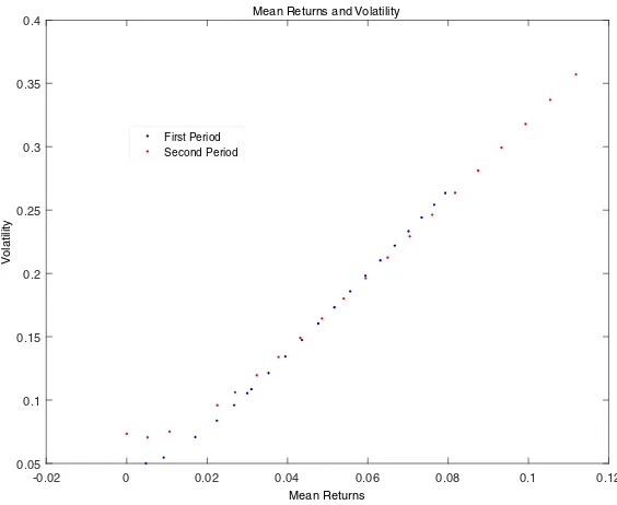
Additionally, we present in Figs. 9 and 10 the mean returns targeted in each period against the random drift and the volatility, respectively, for both periods. We observe a tradeoff between the deterministic and random drift and the volatility cost incurred for higher mean returns.

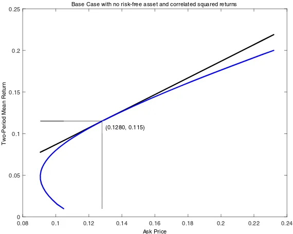
In the absence of access to skewness or whenθ equals zero for each period, the

mean ask price frontier in the absence of a riskless asset is more curved. Figure 11 presents an example of such a frontier.

Two-period mean-variance analysis

For a mean-variance analysis of two-period returns we develop the equations for the two-period mean return and its variance.

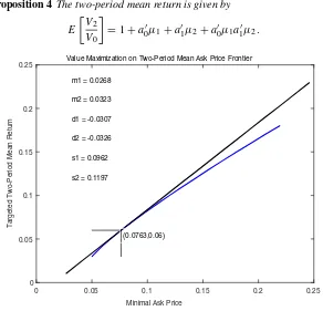
Proposition 4The two-period mean return is given by

E

V2 V0

=1+a₀μ1+a₁μ2+a₀μ1a₁μ2. (7)

0 0.05 0.1 0.15 0.2 0.25

Minimal Ask Price 0

0.05 0.1 0.15 0.2 0.25

nr

ut

e

R

n

a

e

M

d

oir

e

P-o

w

T

d

et

e

gr

a

T

Value Maximization on Two-Period Mean Ask Price Frontier

(0.0763,0.06) m1 = 0.0268

m2 = 0.0323

d1 = -0.0307

d2 = -0.0326

s1 = 0.0962

s2 = 0.1197

-0.02 0 0.02 0.04 0.06 0.08 0.1 0.12 Mean Returns

-0.12 -0.1 -0.08 -0.06 -0.04 -0.02 0

stf

ir

D

m

o

d

n

a

R

Deterministic and Random Drifts

First Period

Second Period

Fig. 9 The random drift as a function of the deterministic drift targeted in each period

-0.02 0 0.02 0.04 0.06 0.08 0.1 0.12

Mean Returns

0.05 0.1 0.15 0.2 0.25 0.3 0.35 0.4

ytil

it

al

o

V

Mean Returns and Volatility

First Period Second Period

0.08 0.1 0.12 0.14 0.16 0.18 0.2 0.22 0.24

Ask Price

0 0.05 0.1 0.15 0.2 0.25

nr

ut

e

R

n

a

e

M

d

oir

e

P-o

w

T

Base Case with no risk-free asset and correlated squared returns

(0.1280, 0.115)

Fig. 11 Mean ask price two-period frontier for correlated squared returns and no random drifts or

skewness access

The variance of the two-period return is given by

V ariance

V2 V0

= a₀1a0+a₁2a1

+a₀1a0a12a1(1+ν (α1∧α2)) (8) +2a₀1a0μ₂a1+2a₁2a1μ₁a0.

We may observe from Eq. (8) that variances over two periods rise with an increase in the share or variance rate of the component in the time change. From a mean-variance perspective one would expect portfolio adjustments to take place within periods in response to such movements in the joint distribution between periods. Let

χ=(1+ν(α1∧α2))be the parameter representing henceforth the dependency in the

time change. The two-period mean-variance optimization problem in the presence of correlated time changes may then be written, for a risk aversion coefficient ofA,as

maximizing over choices ofa0, a1,the objective utilityU,

U=a₀μ1+a1μ2+a0μ1μ2a1−A₂

a₀1a01+2μ2a1+a12a11+2μ1a0 +χ a₀1a0a12a1

(9) subject to the constraints

a₀1 =1 (10)

The impact ofχon portfolio choices in the two periods may be expressed in terms

of positions on the two mean-variance efficiency frontiers for the two single periods. For this purpose, we introduce the two frontiers defined by their distinguished span-ning portfolios (Skiadas (2009)), the minimum variance portfoliosζ1, ζ2 for each

period and two distinguished efficient portfoliosη1, η2that we shall refer to as the

market portfolios for the two periods. These portfolios are given by

ζ1 = −1

1 1

1₁−11

ζ2 = −1

2 1

1₂−11

η1 = −1 1 μ1

1₁−1μ1

η2 = −1 2 μ2

1₂−1μ2 .

In addition, we introduce the variancesσ₁2, σ₂2 and mean returnsw1, w2 on the

minimum variance portfolios as

σ₁2 = 1

1₁−11

σ₂2 = 1

1₂−11

w1 = 1 −1

1 μ1

1−₁11

w2 = 1 −1

2 μ2

1−₂11 .

The mean returnsρ1, ρ2on the market portfolios are given by

ρ1 = μ 11−1μ1

1−₁1μ1

ρ2 = μ 22−1μ2

1−₂1μ2 .

Letm1, v1 andm2, v2 be the mean and variance of two mean-variance efficient

(m1−w1)2 v1−σ12

= w1

σ₁2 (ρ1−w1) (12)

(m2−w2)2 v2−σ22

= w2

σ₂2 (ρ2−w2) . (13)

Proposition 5The solution to the two-period mean-variance optimization

prob-lem of maximizing U as given by Eq.(9)subject to the constraints(10)and(11)is given by two mean-variance efficient portfolios in the two periods satisfying Eqs.(12)

and(13), where the two variances are given by solutions to

v1 =σ₁2+w1(ρ1−w1)

σ₁2 ×

⎛ ⎜ ⎜ ⎝

1+w2+w_σ22

2 (ρ2−w2)

v2−σ₂2−Av2

A

1₊2

w2+

_w

2

σ₂2(ρ2−w2)(v2−σ

2 2)

+χ v2 ⎞ ⎟ ⎟ ⎠ 2 (14)

v2 =σ22+

w2(ρ2−w2)

σ₂2 ×

⎛ ⎜ ⎜ ⎝

1₊w1+ _w

1

σ₁2(ρ1−w1)

v1−σ₁2−Av1

A

1+2

w1+w_σ12

1(ρ1−w1)(v1−σ 2 1)

+χ v1 ⎞ ⎟ ⎟ ⎠ 2 . (15)

The Eqs. (14) and (15) may be solved simultaneously for the volatilities of the two periods with portfolio selections then on the appropriate frontiers. Consider, as an example, a stable frontier across the two periods withw1=w2=.02, σ1=σ2= .05, ρ1=ρ2=.07.

For fixed levels of dependencyχ , we let risk aversion range from 1 to 5. We

graph in Fig. 12 the frontier volatility as a function of risk aversion for two levels of dependence in variance as given byχ.

Additionally, we report the common single-period volatility as a solution to a one-period problem held in each one-period and the common two-one-period volatility (given a stable frontier) held in each period for different values ofχ and comparable risk

aversions.

A single period χ=1.25 χ=1.75

1 0.6344 0.5073 0.4818

3 0.2167 0.2057 0.2027

5 0.1360 0.1330 0.1321

1 2 3 4 5 6 7 8 9 10

Risk Aversion 0.1

0.2 0.3 0.4 0.5 0.6 0.7 0.8

Two-Period Volatility

Two-Period Volatility vs risk aversion for two levels of chi

chi = 1.1

chi = 4

Fig. 12 Frontier volatility as a function of risk aversion for two levels of covariance between random

variances for the two periods

1 1.2 1.4 1.6 1.8 2 2.2 2.4 2.6 2.8 3

Risk Aversion 0

0.1 0.2 0.3 0.4 0.5 0.6 0.7 0.8

Volatility

Common Single-Period and Two-Period Volatility for two chi levels

common single-period volatility for chi = 1.2

two-period volatility for chi = 1.2

two-period volatility for chi = 1.8

We observe a reduction in the single-period volatility exposures taken up in the context of correlation in squared returns across periods.

Apart from the solution of the utility maximization problem for the two-period mean-variance problem, one may take up the direct construction of the two-period mean-variance frontier. Here we wish to minimize the two-period varianceVsubject to attaining a given two-period mean returnm.Hence, we wish to minimize over

choicesa0, a1

V =a₀1a0+a12a1+χ a01a0a12a1+2a01a0μ2a1+2a12a1μ1a0

subject to

a₀1= 1

a₁1= 1

a₀μ1+a₁μ2+a₀μ1μ₂a1 = m.

Proposition 6The solution of the two-period mean-variance frontier lies on the

two single-period efficiency frontiers.

Recognizing that the solution lies on the two single-period frontiers, we may rewrite the problem as one of finding single-period variancesv1,v2to minimize

V =v1+v2+χ v1v2+2v1m2+2v2m1.

subject to

m1+m2+m1m2=m,

where

m1 = w1+

w1

σ₁2 (ρ1−w1)

v1−σ₁2

m2 = w2+

w2

σ₂2 (ρ2−w2)

v2−σ₂2.

Taking the Lagrange multiplierλof the two-period mean constraint as the free

variable in place ofm,we may describe the solution in terms ofλ.

Proposition 7The system of equations for single-period variances for a

v1 = σ₁2+ λ 2

4w1

σ₁2(ρ1−w1) × ⎛ ⎜ ⎜ ⎝

1+w2+ _w

2

σ₂2(ρ2−w2)

v2−σ22

w1

σ₁2(ρ1−w1)

1+2

w2+w_σ22

2 (ρ2−w2)

v2−σ₂2+χ v2 ⎞ ⎟ ⎟ ⎠ 2 (16)

v2 = σ₂2+ λ 2

4w2

σ₂2(ρ2−w2) × ⎛ ⎜ ⎜ ⎝

1₊w1+ _w

1

σ₁2(ρ1−w1)

v1−σ₁2w_σ22

2 (ρ2−w2)

1+2

w1+

_w

1

σ₁2(ρ1−w1)

v1−σ12

+χ v1 ⎞ ⎟ ⎟ ⎠ 2 . (17)

To construct the frontier and the associated solutions we solve Eqs. (16) and (17) for various values ofλand then constructm1, m2andmfrom the equations for the

single-period frontier and the constraint equation form.We may then graph against mthe values forv1, v2. Figure 14 presents a graph of the mean-variance frontiers

for the two periods at two different settings forχ. The parameters used werew1 = .02, w2=.01, σ1=.05, σ2=.03, ρ1=.07, ρ2=.06.

0 0.05 0.1 0.15 0.2 0.25 0.3

Variance 0 0.1 0.2 0.3 0.4 0.5 0.6 0.7 0.8 nr ut e R n a e M d oir e P-o w T

Two-Period Mean Variance Frontiers

var 1 chi =2

var 2 chi =2

var 1 chi =3

var 2 chi =3

In the presence of risk-free assets in the two periods with risk-free returns ofr1, r2,respectively, the two-period mean return is

E

V2 V0

=

⎛

⎝r1a₁(μ2−r21)+r2a₀ 1(μ+1r−1r+11r)2++ar₀1r(μ2+1−r11)+a₁(μ2−r21)

+a₀(μ1−r11) (μ2−r21)a1

⎞ ⎠.

The two-period variance is given by

V ar

V2 V0

=(1+r2)2a₀1a0+(1+r1)2a₁2a1+χ a₀1a0a₁2a1

+2(1+r2) a01a0a1(μ2−r21)+2(1+r1) a12a1a0(μ1−r11) +a₁r21a₀1a0a₁r21−2a₁μ2+a₀r11a₁2a1a₀r11−2a₀μ1.

The portfolios again lie on the single-period mean-variance frontiers which are now linear and described by

x1 = p1s1 x2 = p2s2,

wherexi=mi−riis the excess return on the portfolio andsiis the standard deviation

of the portfolio return. The slope coefficientspiare given by

pi =

1_i−1(μi−ri1) φi

φi = ξi(μi−ri1)

ξi =

_i−1(μi−ri1)

1−_i1(μi−ri1)

.

Conclusion

Portfolio theory for two periods is developed in a context allowing for substantial lev-els of correlation in squared returns while returns are uncorrelated. The returns must then, of necessity, be non-Gaussian making mean-variance analysis less relevant. We develop the two-period conic portfolio problem that leads to a mean ask price frontier. Ask prices are computed using concave distortions and the theory is illustrated and implemented in the context of access to skewness via randomized drifts. The result-ing mean-variance frontier is three-dimensional, expressresult-ing the minimal variance as a function of the targeted levels for the deterministic and random drift. Optimal port-folios maximize a conservative market value seen as a bid price for the portfolio. On the mean ask price frontier, examples illustrate a trade-off between the deterministic and random drifts and the volatility costs of increasing the deterministic drift.

Appendix

Proof of Proposition 1 The Lagrangian is

L=1₂aa−λaμ−m−κaθ−d−πa1−1.

The first order condition is

a=λμ+κθ+π1

with

a=λ−1μ+κ−1θ+π −11.

In terms of the distinguished portfolios (6), we may write

a=λη+κδ+π ζ.

The constraints yield

m=λρη−ρζ

+κρδ−ρζ

+ρζ

d =λyη−yζ

+κyδ−yζ

+yζ

π = 1−λ−κ.

In this case, we have that

v∗=λ2ση2+κ2σδ2+π2σζ2+2λκσηδ+2λπ σηζ +2κπ σδζ.

Proof of Proposition 2With a risk-free asset we have the Lagrangian

L=1₂aa−λa(μ−r1)−m−κaθ−d.

The first order condition is

a−λ (μ−r1)−κθ =0.

Therefore we have that

a=λ−1(μ−r1)+κ−1θ.

In terms of standardized portfolios we may write

a =λξ+κδ

ξ =

−1_(μ−r1)

1−1(μ−r1)

δ =

−1_θ

1−1θ

Hencem, dcan be written in the form

m=λxξ+κxδ

d =λyξ+κyδ,

where

xξ = ξ(μ−r1);xδ=δ(μ−r1)

yξ = ξθ;yδ =δθ.

Proof of Proposition 3The variance ofY1is

σ_Y2₁ = EY₁2−(E[Y1])2

= 3σ₁4−σ₁4

= 2σ₁4.

The variance ofY2is similarly

σY22 =E

Y₂2

−(E[Y2])2

=E

ω+βσ₁2+ασ₁2Z2₁2Z₂4

−ω+(α+β) σ₁22.

We expand the first term to get

ω+βσ₁22+2ασ₁2ω+βσ₁2Z₁2+α2σ₁4Z₁4

Z₂4.

Taking expectations we get

3ω+βσ₁22+6ασ₁2ω+βσ₁2+9α2σ₁4.

We have to subtract

ω+βσ₁2+ασ₁2 2

= ω+βσ₁22+2ω+βσ₁2ασ₁2+α2σ₁4.

Hence

σ_Y2₂ =2ω+βσ₁22+4ω+βσ₁2ασ₁2+8α2σ₁4

=2ω2+4ωβσ₁2+2β2σ₁4+4ωασ₁2+4αβσ₁4+8α2σ₁4

=ω2ω+4(α+β)σ₁2+2β2σ₁4+4ασ₁4(2α+β) .

The denominator for the correlation is then given by

Consider now the covariance computed as the expectation of the productY1Y2less

the product of expectations. The product of expectations is given by

σ₁2ω+(α+β) σ₁2

= ωσ₁2+(α+β) σ₁4.

For the expectation of the product we have

Y1Y2 =σ₁2Z₁2

ω+βσ₁2+ασ₁2Z2₁

Z2₂

=ωσ₁2Z₁2Z2₂+βσ₁4Z₁2Z₂2+ασ₁4Z₁4Z2₂.

Taking expectations we have

ωσ₁2+βσ₁4+3ασ₁4

= ωσ₁2+(α+β) σ₁4+2ασ₁4.

The covariance is then

2ασ₁4,

and the correlation is

ρ = 2ασ

4 1

2σ₁4ω2ω+4(α+β) σ₁2+2β2σ₁4+4ασ₁4(2α+β)

= α

ω2 σ₁4 +

2(α+β)ω

σ₁2 +β

2_{+2α (2α+β)}

≤ α

β2+2α (2α+β)

= 1

β2

α2+4+2β/α

.

Proof of Proposition 4For the two-period expectation we have

E[V2] = V01+a₀μ1+V0E1+a₀R1a₁R2 = V01+a₀μ1+V0a₁μ2+V0Ea₀R1a₁R2

= V01+a₀μ1+V0a₁μ2+V0Ea₀(X1(T1)+μ1) (X2(T2)+μ2)a1 = V01+a₀μ1+a₁μ2+a₀μ1a₁μ2.

For the variance ofV2/V0we have four terms for V2

V0 =1+a

0R1+a₁R2+a₀R1R₂a1.

First, we evaluate

V ara₀R1 = V ara0X1(T1) = E[T1]a₀1a0.

Second, we have

V ara₁R2=E[T2]a₁2a1.

The third variance is

V ara₀R1R₂a1 = Ea₀X1(T1)2X2(T2)a12

= a₀1a0a₁2a1E[T1T2]

= a₀1a0a12a1(1+ν (α1∧α2)) .

Note on taking for unit time,E[T1] =E[T2] =1 that

E[T1T2] = E[(G(α1)+G1(1−α1)) (G(α2)+G2(1−α2))]

= E[G(α1)G(α2)+α1(1−α2)+α2(1−α1)+(1−α1)(1−α2)]

= α1α2+ν(α1∧α2)+α1(1−α2)+α2(1−α1)+(1−α1)(1−α2) = 1+ν (α1∧α2) .

The nonzero covariances are those of

a₀R1, a0R1R2a1,

and also the covariance of

a₁R2, a0R1R2a1.

For the first, we have to consider the product of

a₀X1(T1), a₀R1R₂a1−a₀μ1μ₂a1.

So we have the product of

a₀X1(T1), a0((μ1+X1(T1))(μ2+X2(T2))a1−a0μ1μ2a1

or

a₀X1(T1)2X2(T2)a1+(a0X1(T1))2μ2a1+a0X1(T1)a0μ1X2(T2)a1.

The expectation of this term is using conditional independence ofX1, X2given T1, T2

a₀1a0μ2a1.

Similarly, we have

a₁2a1μ₁a0.

Hence, the variance ofV2/V0is given by (8).

Proof of Proposition 5The first order conditions are for Lagrange multipliersλ0, λ1

for the two constraints

μ1+μ₂a1μ1−Aa₁2a1μ1−A1+2μ₂a11a0−Aχ a₁2a11a0−λ01= 0

or

1+μ₂a1−Aa₁2a1μ1−λ01= A1+2μ₂a1+χ a₁2a11a0

1+μ₁a0−Aa₀1a0μ2−λ11= A1+2μ₁a0+χ a₀1a02a1.

In particular, premultiplying respectively bya₀, a₁

1+μ₂a1−Aa₁2a1a₀μ1−λ0 = A1+2μ₂a1+χ a₁2a1a₀1a0

1+μ₁a0−Aa₀1a0a₁μ2−λ1 = A1+2μ₁a0+χ a₀1a0a₁2a1.

So

λ0 = 1+μ₂a1−Aa₁2a1a₀μ1−A1+2μ₂a1+χ a₁2a1a₀1a0 λ1 = 1+μ₁a0−Aa₀1a0a₁μ2−A1+2μ₁a0+χ a₀1a0a₁2a1.

We may rewrite in terms of first- and second-period meansm1, m2and variances v1, v2defined as

m1 = a₀μ1; m2=a₁μ2 v1 = a01a0; v2=a12a1,

that

λ0 = (1+m2−Av2) m1−A (1+2m2+χ v2) v1 λ1 = (1+m1−Av1) m2−A (1+2m1+χ v1) v2.

Substituting back forλ0, λ1into the first order conditions we get

(1+m2−Av2) μ1+(A (1+2m2+χ v2) v1−(1+m2−Av2) m1)1 =A (1+2m2+χ v2) 1a0

(1+m1−Av1) μ2+(A (1+2m1+χ v1) v2−(1+m1−Av1) m2)1 =A (1+2m1+χ v1) 2a1,

or

a0 = 1+m2−Av2 A (1+2m2+χ v2)

−1 1 μ1+

v1−(1+m2−Av2) m1 A (1+2m2+χ v2)

₁−11

a1 = 1+m1−Av1 A (1+2m1+χ v1)

−1 2 μ2+

v2−(1+m1−Av1) m2 A (1+2m1+χ v1)

₂−11.

It follows that the positions in each period lie on the mean-variance efficient frontiers for each period.

We may then expressa0, a1in terms of standard portfolios as

a0 = (1+m2−Av2) A (1+2m2+χ v2)

w1 σ₁2η1+

v1 σ₁2−

(1+m2−Av2) A(1+2m2+χ v2)

m1 σ₁2

ζ1 (18)

a1 = (1+m1−Av1) A(1+2m1+χ v1)

w2 σ₂2η2+

v2 σ₂2 −

(1+m1−Av1) A(1+2m1+χ v1)

m2 σ₂2

On premultiplication by1we see that the portfolio weights sum to unity.

(1+m2−Av2) A (1+2m2+χ v2)

w1 σ₁2 +

v1 σ₁2 −

(1+m2−Av2) A (1+2m2+χ v2)

m1 σ₁2 = 1 (1+m1−Av1)

A (1+2m1+χ v1) w2 σ₂2 +

v2 σ₂2 −

(1+m1−Av1) A (1+2m1+χ v1)

m2 σ₂2 = 1.

Hence,

v1 = σ₁2+ (1+m2−Av2)

A (1+2m2+χ v2)(m1−w1)

v2 = σ22+

(1+m1−Av1)

A (1+2m1+χ v1)(m2−w2) .

Furthermore, deleting period subscripts, we have that the excess return on any one-period mean-variance efficient portfolio satisfies

m−w=p(ρ−w),

whereρis the mean return onη,the market portfolio given by

ρ= μ −1_μ

1−1μ,

and the mean-variance efficient portfolio in question is

pη+(1−p)ζ.

Fora0, a1the value forpis given in Eq. (18), and hence

m1−w1 = (1+m2−Av2) A (1+2m2+χ v2)

w1

σ₁2(ρ1−w1) (19)

m2−w2 = (1+m1−Av1) A (1+2m1+χ v1)

w2

σ₂2(ρ2−w2) . (20)

We next observe that for any set of mean-variance efficient portfolios we have that

(m1−w1)2

v1−σ₁2 = w1

σ₁2 (ρ1−w1)

(m2−w2)2

v2−σ₂2 = w2

σ₂2 (ρ2−w2) .

As an aside we recall, again now deleting time subscripts, that on any efficient frontier portfolio with weightsω,we have

ω=pη+(1−p)ζ,

hence the meanmofωis

m=pρ+(1−p)w,

or that

m−w=p(ρ−w),