Classification of wood surfaces according to visual appearance by multivariate analysis of wood feature data

(1)

O R I G I N A L A R T I C L E

Classification of wood surfaces according to visual appearance

by multivariate analysis of wood feature data

Lorenz Breinig•_{Rainer Leonhart}•_{Olof Broman}• Andreas Manuel•_{Franka Bru¨chert}•

Gero Becker

Received: 10 January 2014 / Accepted: 24 May 2014 / Published online: 5 December 2014 The Japan Wood Research Society 2014

Abstract Its natural aesthetics make wood an attractive material for construction and design. However, there is no detailed understanding of the relationships between human perception of the appearance and measurable features of wood surfaces that could be used for controlling sawn timber production. This study investigated whether wood surfaces can be classified according to their visual appearance on the basis of wood feature measurements. Cluster analysis was used to discover a classification based on a set of feature pattern variables in a sample of 300 softwood floorboards. A finely graded visual appearance sorting provided a reference. Discriminant analysis was applied to identify the relevant variables from the tested set and to assess predictability of the classification. The results indicated that visual appearance sorting could be approxi-mated quite well by the variable-based classification after

pregrouping according to board position in the log. Ambivalent results were obtained for group prediction within the validation sample. While for boards from some groups prediction was mostly or entirely correct, boards from other groups were largely misclassified. An effect of the available sample was one of the surmised causes, making repetition of the analysis based on a larger sample a desirable focus of further research.

Keywords Wood appearanceWood feature measurementSawn timber sorting Multivariate classification

Introduction

Wood is appreciated as a material for construction and interior design not only for its technical properties but also for its natural aesthetics. Yet so far, only a limited number of studies have investigated the aesthetic perception of wood and the relationships between people’s preference and visible wood properties (e.g. Broman [1], Bumgardner et al. [2], Donovan and Nicholls [3], Nyrud et al. [4], Høibø and Nyrud [5], Nicholls and Barber [6]). In various inter-view studies in Scandinavia, Broman [1] found that dif-fering preferences existed among people and that the most decisive characteristics of a wood surface were the pre-sence of mismatching features and the overall mixture of features. Similar to those findings, Nyrud et al. [4] con-cluded that consumers prefer wood surfaces with homog-enous visual appearance when they investigated the attributes influencing preference for residential decks made of different wood materials. Høibø and Nyrud [5] studied the relationships between preference and visual homoge-neity of wood surfaces. According to their multivariate This paper has been presented at the International IUFRO Conference

‘‘Measurement methods and Modelling approaches for predicting desirable future Wood properties’’ (MeMoWood) held in Nancy, France, 1–4 October 2013.

L. Breinig (&)F. Bru¨chert

Forest Research Institute of Baden-Wu¨rttemberg, Wonnhaldestraße 4, 79100 Freiburg, Germany e-mail: [email protected]

R. Leonhart

Institute of Psychology, University of Freiburg, Engelbergerstraße 41, 79085 Freiburg, Germany

O. Broman

Division of Wood Science and Engineering, Lulea˚ University of Technology, Forskargatan 1, 931 87 Skelleftea˚, Sweden

A. ManuelG. Becker

(2)

models, knot properties had a major influence on the per-ceived homogeneity and thus the attractiveness of a wood surface. In a study on secondary products from Alaska birch lumber, Donovan and Nicholls [3] stated that natural wood features like, e.g. knots were a desired characteristic of wooden products that was even reflected in a higher willingness to pay. By contrast to those findings indicating differentiated preference of consumers, most appearance grading standards or producer-specific rules classify sawn products solely according to the overall degree of wood features with their absence generally rated as highest quality (e.g. Anonymous [7]).

X-ray computed tomography (CT) has for some time been regarded as the most feasible method of roundwood scanning for internal properties (e.g. Taylor et al. [8], Funt and Bryant [9], Grundberg [10]) and recent development has made this technology commercially available (Giu-diceandrea et al. [11]). Various studies have shown that optimization of initial log breakdown based on knowledge of internal wood features—knots in the tested cases— could considerably improve value recovery in sawn tim-ber production (e.g. Rinnhofer et al. [12], Berglund et al. [13]).

Broman [1] noted, in an investigation on the connections between people’s preferences of wood and measurable wood features, that perceptions and preferences of knotty Scots pine (Pinus sylvestris L.) edge glued panel surfaces could to some extent be predicted from wood feature variables by partial least squares (PLS) regression models. Considering these findings and the still evolving prac-ticability of log CT scanning, it can be assumed that uti-lization of this technology to optimize log breakdown according to aesthetic visual appearance of the sawn pro-ducts might hold some potential for increased added value in the wood processing industry. Like any optimization system, such a CT-scanning based sawing optimization for aesthetic quality would require the respective rules to be applied to the detected inner log features.

Thus, the establishment of aesthetic grades expressed through a set of rules for the pattern of features detectable with CT scanning—i.e. mainly knots as this is the most frequent wood feature determining the visual appearance of a wooden piece to a high degree and usually most readily recognized by people—on a board face is a prerequisite, along with knowledge about the valuation of these aes-thetic grades by potential customers. The former in turn translated into the tasks:

1. To investigate if a board classification can be derived from feature pattern measurements on board faces that reproduces or resembles a manual board sorting according to visual appearance to a sufficient extent and

2. To identify the most relevant feature pattern variables together with limits for class distinction and to assess the predictability of the classification found.

This was the overall objective of the present work, while capturing the valuation of different aesthetic appearances was subject to complementary research.

Materials and methods

Sample material and processing

A sample of 58 Norway spruce (Picea abies [L.] Karst.) sawlogs with lengths between 3.9 and 4.2 m and top diameters ranging from 20 to 58 cm were collected from a stand in southwestern Germany. They were scanned with a MiCROTEC CT.LOGX-ray CT scanner.

The logs were then sawn into boards with a green dimension of 309130 mm2, which yielded 810 boards in total. During breakdown of the logs with a frame saw, the position of each board within the sawing pattern and the log was recorded. This was accomplished by sequentially numbering the cants and boards produced in the first and second saw, respectively, and by measuring rotational angle and offset of the sawing patterns in reference to markings applied to the logs previous to the CT scans.

After kiln-drying, the boards were processed to tongue-and-groove profiled boards with a thickness of 20 mm, an exposed face width of 101 mm and a piece width of 110 mm, and they were treated with a water-based oil finish.

All boards were then fed through an industrial-type board scanner utilizing grayscale line cameras and laser sensors on the board faces and edges and RGB line cam-eras on the board faces. The raw image data of all boards were recorded.

Visual appearance sorting and production of sample boards and images

All 810 boards were visually sorted according to their characteristic appearance. Thereby, neither any public grading standards nor producer-specific grading rules were applied. Instead, different appearance classes were estab-lished by iteratively searching for boards with character-istic visual appearance and grouping them with similar ones. If an initial appearance class was not supported by a sufficient number of similar boards or later perceived as not distinct enough from another one, it would be dismissed and the boards would be reassigned to the best matching appearance class. In this iterative sorting procedure, size, condition, shape and distribution of knots, direction of the

(3)

Fig. 1 Panels composed of sample boards from the 15 appearance classes.Each panel contains ten boards from one class. Class numbers are indicated

(4)

annual rings, i.e. flat or vertical grain, colour—which was often influenced by the presence of compression wood—as well as presence and length of visible pith sections were regarded, and all sorting decisions were made by consent of two persons (two of the authors; neither of them being trained as lumber grader). A basic sorting requirement was that the section of characteristic appearance within the board had a minimum length of two metres without any technical defect (such as a knot hole or a large resin pocket) precluding the usability of the piece as a floor or panelling board. Boards that did not have a usable section of at least 2 m length were rejected. When sorting was completed, 15 different visual appearance classes had been established. Board counts differed considerably among these appearance classes.

For each of the 15 appearance classes, 2-m sections of ten boards were selected as representative samples for further use, including studies on people’s preferences for the different visual appearances. They were physically cross-cut from the full-length boards with their exact position within the respective board being documented, and they were composed into panels. The RGB images of the faces of these 150 boards were cropped so that they cor-responded to the decking surfaces of the physical board sections. They were used as the analysis sample in the present study. In addition, another 150 images corre-sponding to 2-m sections, again ten for each of the 15 classes, were produced to use them as a validation sample. Mostly, these images were prepared from images of dif-ferent full-length boards than those used in the analysis sample. However, from 14 boards in the analysis sample, one to four sections at different longitudinal positions within the full-length board (19 sections in total) were also taken for the validation sample. In Fig.1, the samples of the 15 appearance classes, corresponding to the physical board panels, are illustrated.

Knot data acquisition and processing

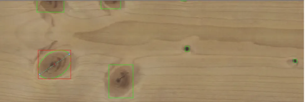
A purpose-built software application was used to obtain measurements of the position and size of knots and pith streaks from the 300 RGB images of the boards. Therefore, one image at a time was loaded and displayed by the application, and, if present on the board face, knots and pith streaks were manually marked by fitting an ellipse to their circumference. X and Y position as well as width and length of the bounding box automatically added by the application during manual marking were saved. Knot condition was assessed and entered as well and a list with all marked features was obtained from the application. Figure2 presents a screenshot of a board image displayed in the user interface.

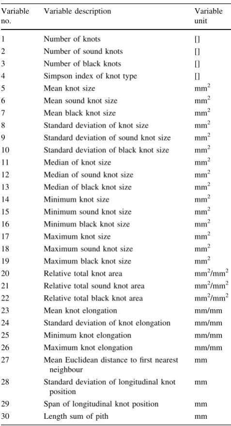
A set of 30 variables describing the knot and pith pattern on the face of each board were calculated from the position and size data of the measured knots and pith streaks. Knot features with a size below 4 mm2were filtered out prior to variable computation since their detection, as sound or black knots, was considered insecure. The variables com-prised knot counts, differentiated by knot type, statistics about knot size and shape distribution, as well as knot dispersion measures and the sum of pith streak lengths. A complete list of all variables is given in Table1.

Determination of expected annual ring pattern

The direction of annual rings on the board faces (i.e. standing annual rings, or vertical grain, versus laying annual rings, or flat grain) was found to be an important

Table 1 Variables calculated from knot and pith measurements on each sample board

Variable no.

Variable description Variable unit

1 Number of knots []

2 Number of sound knots []

3 Number of black knots []

4 Simpson index of knot type []

5 Mean knot size mm2

6 Mean sound knot size mm2

7 Mean black knot size mm2

8 Standard deviation of knot size mm2

9 Standard deviation of sound knot size mm2

10 Standard deviation of black knot size mm2

11 Median of knot size mm2

12 Median of sound knot size mm2

13 Median of black knot size mm2

14 Minimum knot size mm2

15 Minimum sound knot size mm2

16 Minimum black knot size mm2

17 Maximum knot size mm2

18 Maximum sound knot size mm2

19 Maximum black knot size mm2

20 Relative total knot area mm2_/mm2

21 Relative total sound knot area mm2/mm2

22 Relative total black knot area mm2/mm2

23 Mean knot elongation mm/mm

24 Standard deviation of knot elongation mm/mm

25 Minimum knot elongation mm/mm

26 Maximum knot elongation mm/mm

27 Mean Euclidean distance to first nearest neighbour

mm

28 Standard deviation of longitudinal knot position

mm

29 Span of longitudinal knot position mm

30 Length sum of pith mm

(5)

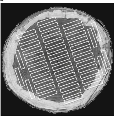
characteristic in the visual sorting, but was not reflected in the variables calculated from the feature measurements on the boards. For this reason, the boards were preclassified according to their expected annual ring pattern by assigning them to three classes, referred to as ‘‘log-sector classes’’, based on their original position in the log. This was done by utilizing the CT data of the logs. First, the actual sawing pattern and its orientation were virtually reconstructed in the CT image of each log, based on the board positions recorded at sawing. Then, for each slice of the CT image, the CT image processing software deter-mined the location of each board in one of the three sectors dividing the log cross-section. The sectors were defined with reference to the log pith and the orientation of the sawing pattern so that they approximately coincided with the different directions of annual rings on the board faces; the scheme is described in Fig.3. For each board, the software registered the sector in which its cross-sec-tion centre was situated on each CT slice and returned the sector with most counts over all slices as the final log-sector class.

Data analysis

Testing the distributions of the individual knot variables for normality revealed deviations from normal distribution in

several cases. Therefore, logarithmic transformation was applied prior to the classification procedure based on multivariate analysis. The classification was then carried out separately for each log-sector class and comprised three main steps:

1. First, an explorative cluster analysis was performed to reveal the natural classification structure within each of the log-sector classes expressed in the knot variables and to assess to which extent a derived classification would coincide with the 15 appearance classes from the visual appearance sorting. Hierarchical-agglomera-tive clustering applying Ward’s minimum variance method on squared Euclidean distances was used (Hair et al. [14]). Separate analyses were done for the boards in the analysis and validation samples. To derive the classifications for further use in the study, the results of the cluster analyses were evaluated by interpreting the dendrograms (cluster trees), i.e. their graphical repre-sentations, and by assessing if the visual appearance of board composition images generated from the single board images according to the established groups was homogeneous, distinct and resembling the original appearance classes.

2. Subsequently (multiple) discriminant analysis (Hair et al. [14]) was conducted for assessing whether any differences between the groups found in each separate

a

b

Fig. 3 aSectors defined on the log cross-section for preclassification of the sample boards according to expected direction of annual rings. The sectors are centred on the pith and aligned with the sawing pattern so that the centre line of sector is parallel to the cutting lines of the first saw. For sideboards, the 1 scheme is rotated 90. The

(6)

cluster analysis were expressed in the variables that would enable predictive classification of further boards. A stepwise estimation of the discriminant function(s) was applied with the objective to identify those variables that were most effective in discrimina-tion of the groups and thus to allow for reducing the number of variables to be used in a future implemen-tation of the classification procedure. Minimum Ma-halanobis distance (D2) and partialF value were used as criteria for variable inclusion or removal. At each step, the variable maximizing the minimum Mahalan-obis distance (D2) between the two closest groups was entered if theFvalue was above the minimum limit for inclusion of 3.84 (corresponding to a significance level

ofa =0.05), and any variable with anFvalue below 2.71 (significance level a=0.1) was removed. Step-wise inclusion was terminated when there were no more variables not already included with F values above 3.84. Each of the estimated discriminant func-tions had the form:

Zjk¼aþC1V1kþC2V2kþ þCnVnk ð1Þ where Zjk is the discriminant score of function j for

observation k, a the constant term, Vik the included

variablei for observationkandCi its coefficient. The

basis for classification was then the scores at the group centroids, i.e. the mean of the scores of the observa-tions within each group that were calculated as:

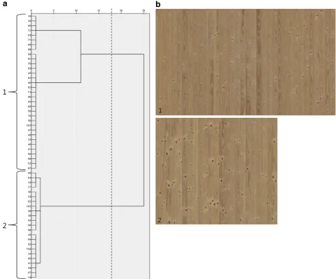
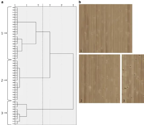
Fig. 4 aDendrogram for the boards from the analysis sample within log-sector class 1 (boards with flat grain). The horizontal scale indicates the distance coefficient, standardized to relative numbers in the interval 0–25, while thenumberson thevertical scaleindicate the

identifiers of the boards. Thedashed lineindicates the chosen cluster solution and the corresponding groups are marked and numbered.

b Compositions of single board images according to the chosen cluster solution labelled with the group numbers

(7)

ZGj ¼ PN

i¼1Zji

N ð2Þ

whereZGjis the score at the centroid of groupj,Zjiis

the score of observation i in group j and N is the number of observations in groupj. In the case of dis-crimination between two groups, a weighted cutting score (ZC) was used for group determination. It was

calculated according to: ZC¼

N1ZG2þN2ZG1 N1þN2

ð3Þ

with N1 and N2 denoting the observation counts in

group 1 and 2, respectively, andZG1and ZG2the scores

at the centroids of the respective groups. In the case when three groups were discriminated by two dis-criminant functions, calculation of a single weighted cutting score for discrimination was not applicable. Instead, for each board to be classified, the Euclidean distance to each of the three group centroid scores in the discriminant functions space had to be calculated. The group of the board would then be determined by the minimum distance. Accuracy of group prediction was evaluated by means of a classification matrix. Thereby, the classification results obtained by applying the discriminant function(s) and cutting scores (group centroid scores) estimated with the analysis sample to

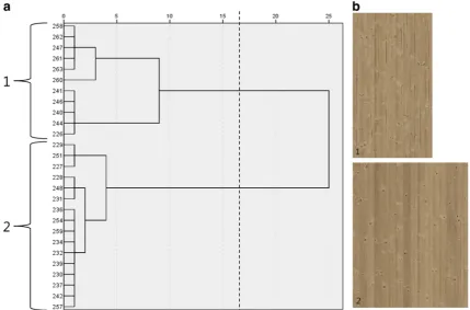
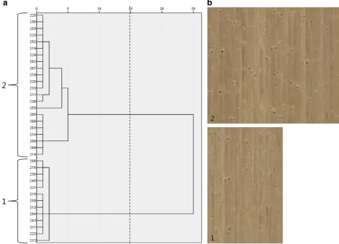
Fig. 5 aDendrogram for the boards from the analysis sample within log-sector class 2 (boards with vertical grain). Thehorizontal scale indicates the distance coefficient, standardized to relative numbers in the interval 0–25, while thenumberson thevertical scaleindicate the

(8)

the validation sample were compared with the original groups of the boards. The results of a cross-validated classification of the analysis sample were included as well. The overall classification result, i.e. the rate of correct group prediction, was assessed by checking whether it was better than proportional chance multi-plied by a factor of 125 %, as proposed by Hair et al. [14]. Press’s Q statistic with the critical value being the quantile of thev2distribution at a significance level of

a =0.01 for one degree of freedom was used for testing whether classification was significantly better than chance (Hair et al. [14]).

3. Hierarchical cluster analysis was then repeated for the analysis and validation sample using only the variables entered in the discriminant functions. It was checked if and to which extent clustering based solely on the reduced set of variables yielded a different classifica-tion compared to the initial cluster analysis.

All analyses were carried out using the SPSS software package, release 22.0.

Results

Some boards could not be considered further in the analysis as their log-sector class could not be determined due to lost data about the position of the individual board in the log. A few boards were excluded from the analysis since they were identified as outliers in the cluster analyses, when considerably larger distances to joining the next cluster compared to the other boards were observable for these boards in the dendrograms. In total, 18 of the boards originally in the analysis sample and 19 of the boards in the validation sample were lost.

Pregrouping of the remaining 132 boards in the analysis sample according to their original position on the log cross-section yielded 56 boards in log-sector class 1 (flat grain as expected annual ring pattern), 49 boards in log-sector class 2 (vertical grain) and 27 boards in log-sector class 3 (boards from the log centre, in parts with exposed pith). For the 131 boards in the validation sample counts were 48, 48 and 35 for log-sector classes 1, 2 and 3, respectively.

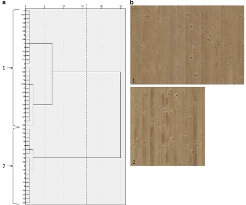
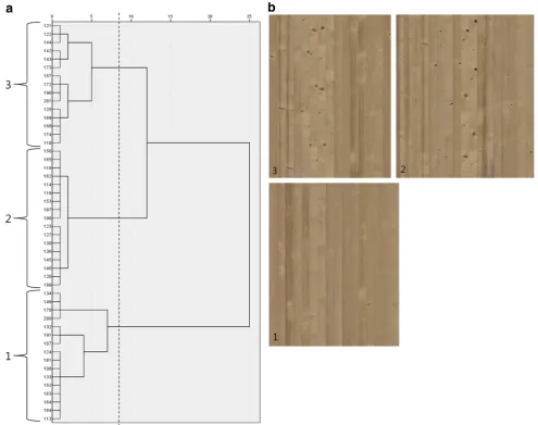
Fig. 6 aDendrogram for the boards from the analysis sample within log-sector class 3 (boards from log centre). The horizontal scale indicates the distance coefficient, standardized to relative numbers in the interval 0–25, while thenumberson thevertical scaleindicate the

(9)

Explorative classification of the pregrouped boards by cluster analysis

Analysis sample

For log-sector class 1 of the analysis sample, the result of the clustering procedure, graphically represented by the dendrogram in Fig.4a, suggested grouping the boards into two or three clusters, or groups. Since there were only comparatively few boards in the first group of the three-cluster solution, making this group less substantial and probably less reproducible, and since a lower group count was generally preferable due to the pregrouping already carried out, the two-cluster solution was chosen for further analysis. The composition images prepared according to the two-cluster solution that are presented in Fig.4b exhibited a contrast between boards with larger sound knots and boards having smaller dead knots, often in a lower number.

A less clear distinction between the meaningful levels of clustering could be observed in the dendrogram resulting from the cluster analysis of log-sector class 2. Here, solu-tions with two, three or four clusters were most distinct as can be seen in Fig.5a. The two-cluster solution obviously entailed very imbalanced board counts among the groups as well as a noticeable variation in the appearance of the

boards in the larger group—joining the boards shown in compositions 1 and 2 in Fig.5b. On the other hand, the four-cluster solution divided the boards contained in group 1 in two groups not exhibiting any important difference in visual appearance and with the problem of likely decreased reproducibility mentioned before. Thus, the three-cluster solution was taken for further analysis as the expectedly most robust classification. Notably, the ten boards com-prised in the small group 3 all belonged to the same ori-ginal appearance sorting class. This congruency together with the large distance of group 3 to the other groups suggested that the visually striking characteristic of these boards—few but large sound knots mostly cut at an angle—was also strongly expressed in the knot variables.

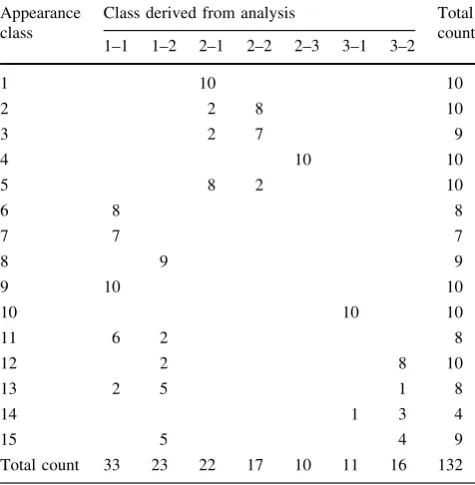
The most pronounced distinction between the groups of the selected clustering solution could be observed for the boards of log-sector class 3, i.e. the boards originating from the log centre. As indicated by the dendrogram in Fig.6a, the two-cluster solution was the obvious basis for sub-sequent investigation. Similar to the case of group 3 within log-sector class 2, all the boards apart from one merged into group 1 had also been assigned to the same class in the appearance sorting. Apparently, variables representing either only the presence of pith streaks or, additionally, some knot properties associated with direct proximity of the pith—e.g. the shape of splay knots or the clustered distri-bution of very small knots—prevailed in the clustering procedure and led to the separation of the boards with visible pith, boards that also formed their proper appearance class. Pregrouping of the boards according to expected direc-tion of annual rings combined with the groups derived from the separate cluster analyses yielded a classification of the boards from the analysis sample into seven classes in total. Thus, the number of classes was reduced by more than half, compared to the original appearance sorting. The agree-ment between these new classes and the original 15 appearance classes was examined with the aid of a cross-table (Table2). It can be noted that some of the appearance classes containing boards with laying annual rings, e.g. classes 12 and 15, were divided at pregrouping, while the boards from other original classes—both with laying and standing annual rings—were dispersed by cluster analysis, as for example classes 2, 5 or 11. Other original appearance classes, on the other hand, were entirely included in one of the new classes, such as class 9, or remained as a distinct class as it was the case with appearance class 4. Unfortu-nately, the majority of boards from appearance class 14 had to be excluded from the analysis due to unavailable or incorrect information on log-sector class, leaving only four out of ten boards in the analysis. The other twelve excluded boards, however, were rather evenly distributed among the appearance classes, so that most of the appearance classes retained at least eight of ten boards.

Table 2 Cross-table indicating coinciding board counts for the ori-ginal visual appearance classification and the classification derived from the explorative analysis for the analysis sample

Appearance class

Class derived from analysis Total count 1–1 1–2 2–1 2–2 2–3 3–1 3–2

1 10 10

2 2 8 10

3 2 7 9

4 10 10

5 8 2 10

6 8 8

7 7 7

8 9 9

9 10 10

10 10 10

11 6 2 8

12 2 8 10

13 2 5 1 8

14 1 3 4

15 5 4 9

Total count 33 23 22 17 10 11 16 132

(10)

Validation sample

The same explorative cluster analyses as for the analysis sample were performed for the validation sample. To enable using the groups from both analysis and validation sample in the subsequent discriminant analysis, numbering of the groups in the clustering solutions chosen for further analysis was synchronized with the numbering of the groups in the analysis sample. Therefore, each group of the validation sample was assigned the same number as the group of the analysis sample most similar in appearance.

When cluster analysis was performed for log-sector class 1 of the boards in the validation sample, the resulting dendrogram (see Fig.7a) indicated—similar to the case of

the boards in the analysis sample—that a two-cluster solution might provide the most meaningful classification of the boards. A three-cluster solution could be identified as producing a classification with balanced counts and little intra-cluster variability as well. However, obtaining the same number of groups, i.e. clusters, as for the boards in the analysis sample was a requirement for the assessment of predictability in the discriminant analysis. Furthermore, taking the two-cluster solution was also justified by the lack of marked visual dissimilarity of the knot patterns between the two first groups of the three-cluster solution. Thus, in the case of log-sector class 1, the hierarchical clustering showed some analogy for the analysis and val-idation samples and the two-cluster solution for the boards

Fig. 7 a Dendrogram for the boards from the validation sample within log-sector class 1 (boards with flat grain). Thehorizontal scale indicates the distance coefficient, standardized to relative numbers in the interval 0–25, while thenumberson thevertical scaleindicate the

(11)

in the validation sample also produced compositions of similar visual appearance, as can be seen in Fig.7b.

By contrast, there were considerable discrepancies between the boards in the analysis and validation samples in the case of log-sector class 2. As Fig.8a shows, a three-cluster solution was distinct for the validation sample as well and therefore deriving the same number of groups for the validation sample as for the analysis sample did not conflict with a feasible interpretation of the cluster tree. However, the visual impression of the derived board compositions markedly differed for two of the three groups. While a group comprising only clear or near knot-free boards was established for the validation sample as well, a good separation between boards with large sound knots and boards with smaller dead knots was not accomplished. As compositions 2 and 3 in Fig.8b

illustrate, boards with predominantly large sound knots and boards with black knots were mixed in those groups with some near clear boards distributed over both.

Applying cluster analysis to the boards in the validation sample in log-sector class 3, on the other hand, again produced a classification that was mostly consistent with the classification of the boards in the analysis sample. As it was the case with the analysis sample, the only feasible solution that could be identified in the dendrogram was at the two-cluster level as indicated by Fig.9a. With a higher number of boards assigned to log-sector class 3 in the validation sample, a complete separation of the boards with pith streaks visible on the face was provided here as well. While for the boards in the analysis sample only one out of eleven boards in group 1 did not belong to the appearance class of pith boards, four out of 13 boards in group 1 of the

Fig. 8 a Dendrogram for the boards from the validation sample within log-sector class 2 (boards with vertical grain). Thehorizontal scale indicates the distance coefficient, standardized to relative numbers in the interval 0–25, while thenumberson thevertical scale

(12)

validation sample were originally assigned to other appearance classes. However, all boards in this cluster actually exhibited pith streaks, albeit of only minor length in the case of one board.

Discriminant analysis of the groups from cluster analysis

Discriminant analysis was then applied to assess whether any differences between the groups found in cluster ana-lysis were expressed in the variables that would enable group prediction. Individual analyses were performed for the groups within each of the log-sector classes.

In the case of log-sector class 1, the data of 56 board images were used in the discriminant analysis and the data of 48 board images were available for validation. After seven iterations, five out of the original 30 variables were included in the discriminant function. The stepwise

procedure is summarized in Table 3, while the standard-ized and non-standardstandard-ized canonical coefficients of the included variables—i.e. the variable weights—and the constant term (intercept) of the discriminant function are listed in Table4. The absolute values of the standardized coefficients indicate the importance of the variables for group discrimination, whereas the non-standardized coef-ficients together with the constant term were used for cal-culation of the discriminant score of each observation according to the discriminant function in Eq.1. The scores at the group centroids, calculated on the basis of the ana-lysis sample, were -7.465 for group 1 and 10.711 for group 2, respectively, which resulted in a weighted cutting score of 3.246. Prediction accuracy was assessed through the classification matrix presented in Table5. While 100 % of the boards in group 2, which corresponded to the clusters comprising boards with larger sound knots, were correctly assigned to this group, only 48.3 % of the boards in group 1

Fig. 9 a Dendrogram for the boards from the validation sample within log-sector class 3 (boards from log centre). Thehorizontal scale indicates the distance coefficient, standardized to relative numbers in the interval 0–25, while thenumberson thevertical scale

indicate the identifiers of the boards. Thedashed lineindicates the chosen cluster solution and the corresponding groups aremarkedand numbered.bCompositions of single board images according to the chosen cluster solution labelled with the group numbers

(13)

were predicted as belonging to that group. With the remaining 51.7 % incorrectly assigned to group 2, the overall rate of correct classification, or hit ratio, was no higher than 68.8 % but still slightly above the applied standard (proportional chance multiplied with 125 %) which corresponded to 65.2 %. The calculated Press’s Q statistic was 6.75 and thereby a little higher than the critical value of 6.63. Despite this overall acceptable result, the poor prediction accuracy for the boards of group 1 had to be regarded as critical since it raised the question whether the discriminant model based on the analysis sample was appropriate for classification of further, yet unknown boards.

For log-sector class 2, the data of the 49 boards in the analysis sample were used for model estimation while the validation sample comprised 48 boards. In the discriminant analysis, 14 iterations were required for the inclusion of twelve variables as shown in Table6. Since cluster ana-lysis lead to three groups within log-sector class 2, the groups that each variable discriminated between are addi-tionally indicated. The canonical coefficients for each of the two discriminant functions and the constant terms are listed in Table 7, and the function values of each dis-criminant function at the group centroids are given in Table8.

As the classification matrix (Table9) shows, the pre-diction results for log-sector class 2 were ambivalent as well. With 93.8 and 94.1 % correct prediction for group 1 and 2, respectively, but all boards from group 3 misclas-sified, overall prediction accuracy was only 64.6 %. Applying the same diagnostics as in the case of the log-sector class 1, it could be noted that—despite the complete misclassification of one group—both the hit ratio was well above the postulated minimum of 41.8 %, and the Press’s Q statistic, with a value of 21.1 compared to the critical value of 6.63, indicated an overall classification signifi-cantly better than chance. However, the total misclassifi-cation of the boards from the validation sample in group 3 had the same implications as the poor prediction accuracy for group 1 of the flat-grain boards, being even more evi-dent in this case.

The likely reason for the misclassification is revealed by the scatter plot in Fig.10. It displays the distribution of the values of the two canonical discriminant functions (discriminant scores) for each board together with the location of the group centroids. As can be seen, many boards of group 3, presumably those from the validation sample, were located very far from their group cen-troid, some of them particularly close to the centroid of group 2.

The boards pregrouped into log-sector class 3 had counts of 27 and 35 boards for the analysis and validation sample, respectively. Group 1 comprised the boards with

Table 3 Variables included or removed in the stepwise discriminant analysis for log-sector class 1

Step Variables Fvalue Minimum

D2 Included Removed

1 Maximum sound knot size

– 860.412 63.482

2 Standard deviation of sound knot size

– 24.414 94.561

3 Simpson index of knot type

– 11.651 116.640

4 Number of sound knots

– 27.505 181.693

5 Relative total sound knot area

– 24.106 271.212

6 Mean sound knot size

– 12.168 339.550

7 – Maximum

sound knot size

1.347 330.357

The partialFvalue and minimumD2_{indicated for each step are the} values computed in the previous step that were the basis for variable inclusion or removal

Table 4 Standardized and non-standardized canonical coefficients of the included variables and intercept of the discriminant function for log-sector class 1

No. Variable Standardized

coefficient

Coefficient

1 Number of sound knots 2.190 4.480

2 Simpson index of knot type -0.912 -17.302

3 Mean sound knot size 2.063 2.794

-1.890 -1.389

5 Relative total sound knot area -1.417 -250.048

Intercept – 4.527

Table 5 Classification matrix for discriminant analysis of the groups resulting from the cluster analyses within log-sector class 1

Actual group Predicted

group

Total

1 2

Analysis sample Cross-validated

Count 1 33 0 33

2 0 23 23

% 1 100.0 0.0 100.0

2 0.0 100.0 100.0

Validation sample

Original Count 1 14 15 29

2 0 19 19

% 1 48.3 51.7 100.0

(14)

visible pith streaks while the remaining boards, mainly characterized by larger sound knots, made up group 2. A set of three variables was included in the discriminant model after three iterations of the stepwise procedure (see Table10for details). The length sum of pith streaks was apparently the most important variable for discrimination between the groups as can be seen from the standardized coefficients listed in Table11together with the non-stan-dardized coefficients and constant term. In this two-group case, discrimination could again be based on a weighted cutting score. With group centroids at function values of 3.968 and -2.728 for group 1 and 2, respectively, this cutting score was 1.24.

Here, group prediction for the boards in the validation sample was entirely correct, as the classification matrix in Table12 shows. Presumably, the complete separation between the boards in both groups on length sum of pith influenced this result. It was noticeable that the cross-val-idated hit ratio of the analysis sample, on the other hand, did not attain 100 %. This was in contrast to the cross-validated hit ratios of the other log-sector classes and might seem surprising given the 100 % prediction result of the validation sample. However, the number of boards pre-dicted as belonging to group 1 equalled the number of boards in the original appearance class comprising the pith boards (ten in either case) and the cross-validation proce-dure therefore actually could have led to a classification of these boards fully consistent with the visual appearance sorting.

Repetition of cluster analysis with reduced sets of variables

The repetition of cluster analysis for the boards from the analysis sample within log-sector class 1, using only the variables included in the discriminant model, modified the dendrogram in that it lead to an even more outstanding two-cluster solution. It thereby caused the reallocation of four boards from group 2 to group 1. These boards had rather small and dark knots, and therefore they were not the most representative ones for group 2. Thus, this reassign-ment could be deemed as a slight improvereassign-ment of the classification, leading to an increased homogeneity within group 2.

By contrast, clustering of the boards of the analysis sample in log-sector class 2 seemed to be adversely affected by variable reduction. The shape of the cluster tree was altered considerably, compared to clustering based on the full set of variables, making the three-cluster level less distinct. Three boards were reallocated from group 3 to group 1 that originally comprised only clear and near clear boards.

It was assumed that the influence of the length sum of pith within log-sector class 3 was already prevailing in cluster analysis based on all variables. This assumption was supported when cluster analysis based on only this and two other included variables produced a cluster tree with an even more distinct two-cluster level. Due to the realloca-tion of one board in the reiterated cluster analysis, group 1

Table 6 Variables included or removed in the stepwise discriminant analysis for log-sector class 2

The partialFvalue and minimumD2indicated for each step are the values computed in the previous step that were the basis for variable inclusion or removal. The groups that each variable separated between are given likewise, i.e. the discriminated groups were always identified in the preceding step as well

D2

Groups discriminated

Included Removed

1 Maximum knot size – 71.029 4.812 1–2

2 Number of knots – 44.332 11.205 1–2

3 Span of longitudinal knot position – 12.476 17.198 2–3

– 28.589 28.333 1–2

5 Mean Euclidean distance to first nearest neighbour

– 31.818 35.875 1–3

6 – Span of longitudinal

knot position

1.613 33.161 1–3

7 Minimum black knot size – 24.121 78.914 1–3

8 Simpson index of knot type – 8.231 82.337 1–2

9 Standard deviation of knot size – 26.453 115.155 2–3

10 Minimum sound knot size – 25.399 207.024 1–2

11 Minimum knot elongation – 4.570 232.143 1–2

12 Standard deviation of black knot size

– 5.432 263.306 1–3

13 Number of black knots – 25.457 405.287 1–2

14 Maximum black knot size – 11.632 527.664 1–2

(15)

was thereby fully congruent with the pith-board class from the visual appearance sorting, which also sustained the assumption that group prediction based on the included discriminant variables lead to a classification of the respective boards consistent with the original sorting. The cluster trees and corresponding board compositions for all three log-sector classes are presented in Figs.11,12,13.

For the boards from the validation sample in log-sector class 1—as it was the case for the analysis sample— repeated cluster analysis with the five variables included in the discriminant model caused reallocation of three boards from group 2 to group 1. Since large sound knots and small black knots were equally present on the faces of the reallocated three boards, this regrouping was neither con-sidered an improvement of the classification nor an impairment. The shape of the dendrogram was not mark-edly altered with the two-cluster level still being most distinct.

With the initial cluster analysis, a visually inhomoge-neous classification of the boards in log-sector class 2 was observed for the validation sample. When cluster analysis was rerun on the basis of the included variables, the reas-signment of nine boards at the three-cluster level indeed

produced a visually homogeneous group of vertical-grain boards with large sound knots (group 3). However, this group comprised only six boards, whereas the large cluster that the boards were allocated to (group 2) contained 26 boards with large variation in appearance. Thus, the board counts in the three groups were very unbalanced and there was only little distance between the three-cluster level and levels with more clusters in the cluster tree—a less distinct three-cluster level due to variable reduction as it could be observed for the vertical-grain boards in the analysis sample as well. On the other hand, the cluster with (near) clear boards (group 1) was not affected by variable reduction; this robustness was also reflected in a large distance to the remaining cluster at the two-cluster level.

Cluster analysis reiterated with the reduced set of vari-ables for the boards in the validation sample in log-sector class 3 did not change the allocation of the boards to the groups at the two-cluster level, when compared with the initial cluster analysis with all variables. The shape of the cluster tree indicated a maximum separation between the two groups probably due to the amplified effect of the length sum of pith after variable reduction. Figures 14,15, 16 show the dendrograms and corresponding board com-positions for all three log-sector classes.

Discussion

The tested classification procedure led to ambivalent results. On the one hand, the classes established by pre-grouping and by subsequent clustering based on all vari-ables had a distinct appearance with quite high within-class homogeneity and could thus be seen as a comparatively

Table 7 Standardized and non-standardized canonical coefficients of the included variables and intercepts of the discriminant functions for log-sector class 2

No. Variable Standardized coefficients Coefficients

Function 1 Function 2 Function 1 Function 2

1 Number of knots -6.276 0.519 -19.856 1.643

2 Number of black knots 5.388 0.817 15.134 2.295

3 Simpson index of knot type 3.944 -2.168 15.859 -8.716

4 Standard deviation of knot size 4.240 -2.305 2.652 -1.441

5 Standard deviation of sound knot size 4.064 -0.398 2.647 -0.260

6 Standard deviation of black knot size -1.018 0.335 -0.883 0.291

7 Minimum sound knot size 2.871 0.264 2.382 0.219

8 Minimum black knot size 3.982 -1.337 2.647 -0.889

9 Maximum knot size 2.430 3.284 1.720 2.324

10 Maximum black knot size -7.383 -1.159 -4.667 -0.733

11 Minimum knot elongation -2.378 0.239 -7.336 0.738

12 Mean Euclidean distance to first nearest neighbour -4.103 2.533 -2.921 1.804

Intercept – – 2.702 -7.390

Table 8 Function values of the two discriminant functions (dis-criminant scores) at the group centroids

Group Group centroids

Function 1 Function 2

1 2.657 -7.257

2 -16.910 4.776

3 22.901 7.847

(16)

good approximation of the visual appearance sorting, albeit with the exception of the boards in the validation sample in log-sector class 2. On the other hand, due to the partly insufficient classification results for log-sector classes 1

and 2 in the validation sample, it seemed questionable whether the variables and discriminant functions found for these two classes are generally applicable, i.e. would allow for a classification of boards consistent with human per-ception of board appearance.

Manual sorting of the boards according to their visual characteristics lead to a large number of classes with a fine gradation of appearance and, as mentioned, considerable differences in class counts. The latter turned out to be

Table 9 Classification matrix for discriminant analysis of the groups resulting from cluster analysis within log-sector class 2

Actual group Predicted group Total

1 2 3

Count 1 22 0 0 22

2 0 17 0 17

3 0 0 10 10

% 1 100.0 0.0 0.0 100.0

2 0.0 100.0 0.0 100.0

3 0.0 0.0 100.0 100.0

Validation sample

Original Count 1 15 0 1 16

2 1 16 0 17

3 5 10 0 15

% 1 93.8 0.0 6.3 100.0

2 5.9 94.1 0.0 100.0

3 33.3 66.7 0.0 100.0

Fig. 10 Distribution of discriminant scores of the boards from log-sector class 2 with group centroids indicated

Table 10 Variables included or removed in the stepwise discrimi-nant analysis for log-sector class 3

D2

Included Removed

1 Length sum of pith – 128.119 19.655

2 Maximum black knot size – 9.263 28.721

3 Relative total knot area – 11.383 44.832

The partialFvalue and minimumD2indicated for each step are the values computed in the previous step that were the basis for variable inclusion or removal

Table 11 Standardized and non-standardized canonical coefficients of the included variables and intercept of the discriminant function for log-sector class 3

No. Variable Standardized coefficient

Coefficient

1 Maximum black knot size -0.813 -0.637

2 Relative total knot area 0.700 131.166

3 Length sum of pith 0.921 0.766

Intercept – -1.559

Table 12 Classification table for discriminant analysis of the groups resulting from the cluster analyses within log-sector class 3

Actual group Predicted group Total

1 2

Count 1 10 1 11

2 0 16 16

% 1 90.9 9.1 100.0

2 0.0 100.0 100.0

Validation sample

Original Count 1 13 0 13

2 0 22 22

% 1 100.0 0.0 100.0

2 0.0 100.0 100.0

(17)

problematic since some appearance classes were repre-sented by only a small number of boards. Very limited choice of boards in these appearance classes made select-ing boards for the validation sample that were not as visually consistent and homogeneous as the boards in the analysis sample unavoidable. In some cases, even two or more virtual two-metre-sections had to be taken from the image of the same full-length board. While this circum-stance might largely explain the poor classification results, it also implied that some appearance classes would only be representative for very small shares of sawn timber production.

The classification results, together with the change of the dendrograms when reiterating the cluster analyses, could also indicate that the board groups derived from the initial cluster analyses were too much of an adaption to the analysis sam-ples, entailing that the discriminant models established on their basis were overfitted as well. Therefore, it should be tested on a preferably large sample whether the classifications found in the cluster analyses could be reproduced and whe-ther discriminant analysis based on this classification would result in similar discriminant models.

There were considerable differences between the sets of variables included in the discriminant models for the indi-vidual log-sector classes. While for log-sector class 1— except for one variable—only variables describing the occurrence of sound knots appeared to be relevant for group discrimination, in the case of log-sector class 2 a large set of different variables was included in the discriminant model. It contained variables related to the size distribution of knots, but also variables describing knot shape and spatial distri-bution. Two variables were included in the discriminant models for both log-sector class 1 and 2. With maximum black knot size, the discriminant model for log-sector class 3 shared one variable with that for log-sector class 2, but it was apparently mainly governed by length sum of pith.

Only those wood features relevant for the visual appear-ance that can already be detected with sufficient accuracy in a CT scan could be taken into account for the creation of the tested variables. The annual ring pattern on the board faces— the most important feature in the visual sorting together with the knot pattern—could be well predicted from the defined log sectors since it is mainly determined by the cut orientation of a board and modified to only a minor extent by the actual shape of the annual rings, i.e. their width and deviation from ideal concentric circles. Still, if reliable measurement of the annual rings was available from CT scans, e.g. for species with usually wider annual rings and strong density contrast between early and late wood, such as Douglas fir (Pseud-otsuga menziesii[Mirb.] Franco), it could be tested whether variables derived from this measurement were suitable for classification instead of pregrouping according to expected annual ring direction. Colour variation and contrast,

especially due to compression wood, on the other hand, could not be expressed in the variables at all, although it also was an important characteristic in the visual appearance sorting as it influenced the formation of two sorting classes, 5 and 7.

(18)

Conclusions

• Visual appearance sorting with a fine gradation of visual characteristics and thus a large number of dif-ferent classes could be reproduced in relatively good approximation with the tested two-stage classification procedure.

• The variables included in the discriminant models differed considerably between the log-sector classes, with no variable being present in all models.

• There might be other variables describing the feature pattern on a wood surface that could improve classification. However, the majority of these variables are not available for sawing optimization utilizing CT data of logs. • Group prediction by means of the discriminant models

did not yield satisfactory accuracy for the validation sample in all cases. This might be explained by some

heterogeneity between analysis and validation sample but could also signify overfitting.

• Due to the limited size of the available sample, any results of this investigation may be taken as indicative only.

• Therefore, further research should include both repeat-ing cluster analysis and verifyrepeat-ing the discriminant models on a preferably large data basis.

Acknowledgments This study was conducted in the framework of a research project supported by contract research ‘‘Internationale Spitzenforschung II/2’’of theBaden-Wu¨rttemberg Stiftung.

Appendix

See Figs.11,12,13,14,15,16.

Fig. 11 aDendrogram for the boards from the analysis sample in log-sector class 1 based on the variables included in the discriminant model. The horizontal scale indicates the distance coefficient, standardized to relative numbers in the interval 0–25, while the numberson thevertical scale indicate the identifiers of the boards.

The dashed line indicates the chosen cluster solution and the corresponding groups aremarkedandnumbered. Boards reallocated from group 2 to group 1 are indicated by the shaded box.

(19)

(20)

The dashed line indicates the chosen cluster solution and the corresponding groups are markedand numbered. The board reallo-cated from group 1 to group 2 is indireallo-cated by the shaded box.

(21)

Fig. 14 aDendrogram for the boards from the validation sample in log-sector class 1 based on the variables included in the discriminant model. The horizontal scale indicates the distance coefficient, standardized to relative numbers in the interval 0–25, while the numberson thevertical scale indicate the identifiers of the boards.

(22)

Fig. 15 aDendrogram for the boards from the validation sample in log-sector class 2 based on the variables included in the discriminant model. The horizontal scale indicates the distance coefficient, standardized to relative numbers in the interval 0–25, while the numberson thevertical scale indicate the identifiers of the boards.

The dashed line indicates the chosen cluster solution and the corresponding groups aremarkedandnumbered. Boards reallocated from group 3 to group 2 are indicated by the shaded boxes.

(23)

Fig. 16 Dendrogram for the boards from the validation sample in log-sector class 3 based on the variables included in the discriminant model. The horizontal scaleindicates the distance coefficient,

standardized to relative numbers in the interval 0–25, while the numberson thevertical scale indicate the identifiers of the boards. Thedashed line indicates the chosen cluster solution and the corresponding groups aremarkedand numbered. No boards have been reallocated; therefore,

presenting the board

(24)

References

1. Broman NO (2000) Means to measure the aesthetic properties of wood. Doctoral thesis 2000:26, Lulea˚ University of Technology, Lulea˚, Sweden

2. Bumgardner MS, Bush RJ, West CD (2001) Knots as incongruent product feature: a demonstration of the potential for character-marked hardwood furniture. J I Wood Sci 15:327–335

3. Donovan G, Nicholls D (2003) Consumer preferences and will-ingness to pay for character-marked cabinets from Alaska birch. Forest Prod J 53:27–32

4. Nyrud AQ, Roos A, Rødbotten M (2008) Product attributes affecting consumer preference for residential deck materials. Can J For Res 38:1385–1396

5. Høibø O, Nyrud AQ (2010) Consumer perception of wood sur-faces: the relationship between stated preferences and visual homogeneity. J Wood Sci 56:276–283

6. Nicholls DL, Barber V (2010) Character-marked red alder lumber from southeastern alaska: profiled panel product preferences by residential customers. Forest Prod J 60:315–321

7. Anonymous (2002) Sawn timber—Appearance grading of soft-woods—Part 1: European spruces, firs, pines, Douglas fir and larches (including amendment 1:2002). EN 1611-1:1999 ?

A1:2002

8. Taylor FW, Wagner FG, McMillin CW, Morgan LL, Hopkins FF (1984) Locating knots by industrial tomography—a feasibility study. Forest Prod J 34:42–46

9. Funt BV, Bryant EC (1987) Detection of internal log defects by automatic interpretation of computer tomography images. Forest Prod J 37:56–62

10. Grundberg S (1999) An X-ray LogScanner: a tool for control of the sawmill process. Doctoral thesis 1999:37, Lulea˚ University of Technology, Lulea˚, Sweden

11. Giudiceandrea F, Ursella E, Vicario E (2011) A high speed CT scanner for the sawmill industry. In: Proceedings of the 17th international non destructive testing and evaluation of wood symposium, University of West Hungary, Sopron, Hungary 12. Rinnhofer A, Petutschnigg A, Andreu JP (2003) Internal log

scanning for optimizing breakdown. Comput Electron Agr 41:7–21

13. Berglund A, Broman O, Gro¨nlund A, Fredriksson M (2013) Improved log rotation using information from a computed tomography scanner. Comput Electron Agr 90:152–158 14. Hair JF, Black CB, Babin BJ, Anderson RE (2010) Multivariate

data analysis. Pearson, New Jersey

15. Farina A (2006) Principles and methods in landscape ecology. Springer, Dordrecht