O R I G I N A L A R T I C L E
One-dimensional numerical solution of the diffusion equation
to describe wood drying: comparison with two- and
three-dimensional solutions
Wilton Pereria da Silva1 •Cleide Maria D. P. S. e Silva1•
Andre´a Fernandes Rodrigues1•Rossana Maria Feitosa de Figueireˆdo1
Received: 11 December 2014 / Accepted: 3 April 2015 / Published online: 28 April 2015 ÓThe Japan Wood Research Society 2015
Abstract This article describes drying of wood cut into parallelepiped shaped pieces. A one-dimensional numerical solution of the diffusion equation with boundary condition of the third kind was proposed to describe the process. The lumber was cut into the following dimensions: thickness
T=36 mm, heightH=100 mm and lengthL =745 mm. The convective drying experiment was carried out with forced air at temperature of 40°C, relative humidity of 40 % and velocity of 3 m s-1. An optimizer was coupled with the proposed numerical solution to determine the process parameters. Comparison of the results obtained in this article (one-dimensional) with results from the lit-erature (two- and three-dimensional) indicated good agreement between the process parameters (and also simulations). However, the optimization time for one-di-mensional model is about 15 times less than the optimiza-tion time for the two-dimensional case.
Keywords Numerical simulationVariable diffusivity
Finite volumeOptimizationLumber
List of symbols
A,B,a,b Coefficients of the discretized diffusion equation or fitting parameters
D Effective mass diffusivity (m2s-1)
H Height of the lumber (m)
L Length of the lumber (m)
M Local moisture content at the instant t
(kgwaterkg1drymatter)
M Average moisture content at instant
t(kgwaterkg1drymatter)
Np Number of experimental points (dimensionless)
N Number of control volumes (dimensionless)
R2 Coefficient of determination (dimensionless)
T Thickness of the lumber (m)
t Time (s)
Dx Thickness of a control volume (m)
ri Standard deviation of the experimental point
i(dimensionless)
v2 Chi square or objective function (dimensionless)
Introduction
In several industrial sectors, several production processes involve a stage in which water is transferred to or removed from the products during their manufacture. Among these production processes, it can be cited those referring to the industry of ceramic materials, pharmaceutical products, foodstuff and wood. For wood, the main operation of water removal is the drying process and, nowadays, the main technique is the use of hot air at given velocity. According to Dincer [1], drying is one of the most important stages in the processing of wood, having an important influence on the quality of the final product. Thus, understanding this process of water removal allows to obtain a dry product with superior quality. In this sense, a mathematical model is usually used to describe wood drying. The more accurate information can be extracted from the model used to de-scribe the process, the better model could be considered. In & Wilton Pereria da Silva
1 Federal University of Campina Grande, Campus I,
the literature, one of models used to describe drying of products is that which describes the water migration by diffusion. Diffusion models are used to describe many types of processing such as cooling [2, 3], heating [4], osmotic dehydration [5], and drying of porous materials [6]. In particular, several works are available in the lit-erature involving diffusion models in the description of wood drying [1, 7–15]. According to Silva et al. [14], an advantage of diffusion models when compared, for exam-ple, with empirical models, is the possibility to determine the moisture distribution within the wood at any instant during drying. This information is essential to identify re-gions prone to warping and cracking formation.
In the literature, several analytical solutions of the dif-fusion equation are used to describe drying processes of wood [1,11,13]. Dincer [1] used a one-dimensional ana-lytical solution for the infinite slab to describe drying of lumber cut in the radial direction all-heartwood specimen of Douglas-fir (Pseudotsuga menziessi (Poir.) Britton). According to the author, a practical experimental moisture content and time data set for a slab wood dried with hot air was used, and the results were reasonable when compared with the results predicted by his model. Ricardez et al. [11] used a two-dimensional analytical solution of the diffusion equation to describe drying of red oak (Quercus spp.) samples at vacuum pressure. The authors concluded that their model was able to reproduce the drying kinetics of wood that occurred in two stages: constant and falling rates. Silva et al. [13] used several analytical models, in-cluding a three-dimensional model to describe drying of lumber (Pinus elliottii Engelm.). The authors concluded that three-dimensional model with boundary condition of the third kind reasonably described the process. However, these authors commented that analytical models normally presuppose restrictive assumptions such as constant vol-ume and effective mass diffusivity. Thus, these authors have suggested in their conclusions that numerical solu-tions instead analytical solusolu-tions should be used to describe wood drying, to avoid those restrictions.
Olek and Weres [12] used the finite element method to solve the one-dimensional diffusion equation in Cartesian coordinates. The authors proposed a variable effective mass diffusivity as a function of the moisture content to use their numerical solution for describing drying of Scots pinewood (Pinus sylvestrisL.). The authors concluded that the best results were obtained for the effective mass dif-fusivity given by an exponential expression in which the exponent is a quadratic function of the moisture content. On the other hand, Silva et al. [14] described convective drying of lumber (Pinus elliottiiEngelm.) at low air tem-perature. Silva et al. [14] described the drying process using a three-dimensional numerical solution of the diffu-sion equation, in which was supposed variable effective
mass diffusivity. The model permitted a rigorous descrip-tion of the drying process, and it can predict the moisture content in any position within the parallelepiped that rep-resents the lumber, at any time. However, Silva et al. [15] observed that the determination of the process parameters through optimization technique, using three-dimensional model, takes a long time to perform. Because of that, these last authors used a two-dimensional numerical solution of the diffusion equation to describe same drying studied by Silva et al. [14]. In this two-dimensional study, Silva et al. [15] reported good results, and the optimization time for their model was about 20 times less than the optimization time with the typical three-dimensional solution. Naturally, in this context, a question should be answered: is the one-dimensional model a good option to describe same drying? In this sense, the aim of this article is defined in the following.
The objective of this article was to describe drying of wood cut into parallelepiped shaped pieces, considering the effective mass diffusivity as a variable property. For this purpose, a numerical solution of the one-dimensional dif-fusion equation was proposed and coupled with an opti-mizer to determine the process parameters. In addition, a second objective was to compare the results obtained herein with other found in the literature supposing the lumber with two- and three-dimensional geometry.
Materials and methods
The one-dimensional diffusion equation in Cartesian co-ordinates, used to describe water migration during drying of lumber can be written as [16]:
oM ot ¼
o ox D
oM ox
; ð1Þ
whereM is the local moisture content (kgwaterkg1drymatter);
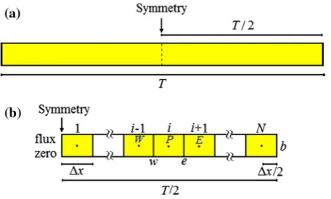
tis the time (s);xis the position (m) within the infinite slab with origin in the center; andDis the effective mass dif-fusivity (m2s-1). The following assumptions were as-sumed to numerically solve Eq. (1): (a) liquid diffusion was considered as the main mass transport mechanism inside the product; (b) the boundary condition is of the third kind; (c) the product was considered homogeneous and isotropic; (d) the diffusion process presents symmetry with respect to the midpoint of the slab.
Numerical solution
N control volumes in a symmetrical piece of the infinite slab, and each control volume has a thickness given by Dx (m). Figure1b also shows an internal control volume ‘‘i’’ with nodal point ‘‘P’’, and its neighbors to west ‘‘W’’ and east ‘‘E’’. The lowercases ‘‘w’’ and ‘‘e’’ refer to the interfaces of the control volume ‘‘P’’ to west and east, respectively.
The integration of Eq. (1) with respect to space (Dx) and time (fromt up to t?Dt), for a control volume P, gives the following result:
MPM0P
Dt Dx¼Ce oM
ox e
CwoM
ox w
ð2Þ
in which the superscript ‘‘0’’ means ‘‘former timet’’ and its absence means ‘‘current timet?Dt’’.
Internal control volumes
For an internal control volume, the following algebraic equation was obtained from the discretization of Eq. (1):
AwMWþApMPþAeME¼B ð3Þ
and the coefficients Aw, Ap, Ae and B are given in Silva et al. [5], where the diffusion equation was discretized for the boundary condition of the first kind. Naturally, for an internal control volume, Eq. (3) is independent of the boundary condition.
Control volume 1
For the control volume 1, the boundary condition was supposed to be of the second kind, with flux zero at west side due to the symmetry. Thus, the following algebraic equation was obtained:
ApMPþAeME¼B: ð4Þ
Again, the coefficientsAp,Aeand Bare given in Silva et al. [5] and, for that, they were omitted herein.
Control volume N
For the control volumeN, the derivatives of Eq. (2) were approximated by:
oM ox w
ffi MPMW
Dx ð5Þ
and
oM ox e
ffi MbMP
Dx=2 ð6Þ
whereMbis the value ofMat the east boundary. Thus, for the control volumeN, the subscript ‘‘e’’ (east) is equivalent to ‘‘b’’ (boundary). The boundary condition of the third kind to east side is expressed by
DoM ox e
¼hbðMbMeqÞ; ð7Þ
in which hbis the convective mass transfer coefficient at east boundary, andMeqis the equilibrium moisture content.
Combining Eqs. (6) and (7) to expressMb, and substituting
Mbinto Eq. (6), this new equation and also Eq. (5) can be used to rewrite Eq. (2). The following algebraic equation is obtained:
AwMWþApMP¼B; ð8Þ
where
Aw¼
1
DxDw; ð9aÞ
AP ¼ Dx
Dtþ Dw Dxþ
Db Db hbþ
Dx 2
; ð9bÞ
B¼Dx
DtM
0 Pþ
Db Db hbþ
Dx 2
Meq: ð9cÞ
In Eq. (9c), M0
P is the moisture content in the control volumePat the beginning of the time step.
Equations (3), (4) and (8) constitute a system of equa-tions in each time step, and such system was solved by the method ‘‘tri-diagonal matrix algorithm’’ [17], also called TDMA. The average value ofMat any instant, denoted by
M, was calculated by a arithmetic average of the moisture contents obtained for the control volumes, once the established grid is uniform.
Effective mass diffusivity
The expression used in this article for the effective mass diffusivity as a function of local moisture content during drying of wood at low temperature was proposed by Silva et al. [14,15], and is given by:
D¼b expða=MÞ; ð10Þ
Fig. 1 aInfinite slab;buniform grid with Ncontrol volumes in a
where ‘‘a’’ and ‘‘b’’ are parameters that fit the numerical solution to an experimental data set. For a uniform grid, on the interfaces of the internal control volumes, for example, ‘‘e’’ (see Fig.1),Dis determined through harmonic mean [16]:
De¼
2DEDP
DEþDP
; ð11Þ
where DP and DE at the nodal points ‘‘P’’ and ‘‘E’’ are calculated through Eq. (10).
As the effective mass diffusivityDis variable, the co-efficientsA in Eqs. (3), (4) and (8), as well as the coeffi-cients B, are calculated in each time step, due to the nonlinearities caused by the variation of such parameter. If the time refinement is adequate, the errors due to the nonlinearities can be discarded.
Optimization
Establishing the function given by Eq. (10) to express the effective mass diffusivity D at the nodal points, the pa-rametersa andb, as well as the convective mass transfer coefficienth, can be determined by optimization. The ex-pression of the Chi square [18,19] was chosen as objective function:
v2¼X
Np
i¼1
Mexpi Msimi
h i21
r2 i
; ð12Þ
in whichMexpi is the average moisture content measured in the experimental point i, Msimi is the correspondent simulated moisture content, Np is the number of ex-perimental points, 1=r2
i is the statistical weight referring to the pointi. According to Silva et al. [20], if the statistical weights are unknown, they can be made equal to a common value, for instance 1. In Eq. (12), it is interesting to observe that the v2 depends on Msimi , which depends on D and
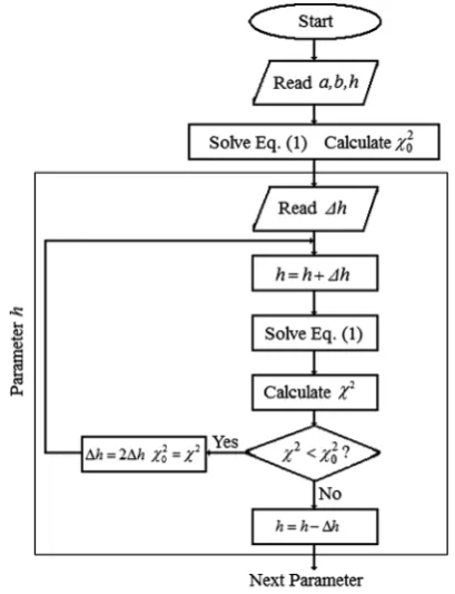
h. Thus, if the convective mass transfer coefficient can be considered constant and the effective mass diffusivity is given by Eq. (10), the parameters ‘‘h’’, ‘‘a’’ and ‘‘b’’ can be determined through the minimization of the objective function, which is accomplished in cycles involving the steps given in the following [3,20].
1. Provide the initial values for the parameters ‘‘a’’, ‘‘b’’ and ‘‘h’’. Solve the diffusion equation and determine thev2;
2. Provide the value for the correction of ‘‘h’’; 3. Correct the parameter ‘‘h’’, maintaining the
pa-rameters ‘‘a’’ and ‘‘b’’ with constant values. Solve the diffusion equation and calculate thev2;
4. Compare the latest calculated value of the v2 with the previous one. If the latest value is smaller, return
to the step 2; otherwise, decrease the last correction of the value of ‘‘h’’ and proceed to step 5;
5. Provide the value for the correction of ‘‘a’’; 6. Correct the parameter ‘‘a’’, maintaining the
pa-rameters ‘‘b’’ and ‘‘h’’ with constant values. Solve the diffusion equation and calculate thev2;
7. Compare the latest calculated value of thev2 with
the previous one. If the latest value is smaller, return to the step 5; otherwise, decrease the last correction of the value of ‘‘a’’ and proceed to step 8;
8. Provide the value for the correction of ‘‘b’’; 9. Correct the parameter ‘‘b’’, maintaining the
pa-rameters ‘‘a’’ and ‘‘h’’ with constant values. Solve the diffusion equation and calculate thev2;
10. Compare the latest calculated value of thev2 with the previous one. If the latest value is smaller, return to the step 8; otherwise, decrease the last correction of the value of ‘‘b’’ and proceed to step 11;
11. Begin a new cycle coming back to the step 2 until the stipulated convergence for the parameters ‘‘a’’, ‘‘b’’ and ‘‘h’’ is reached.
According to Silva et al. [20], in each cycle, the value of the correction of each parameter can be initially modest, compatible with the tolerance of convergence imposed to the problem. For a given cycle, in each return to the step 2, 5 or 8, the value of the new correction can be multiplied by the factor 2. If the modest correction initially informed does not minimize the objective function, in the next cycle, its value can be multiplied by the factor-1.
A simplified flowchart for the optimization algorithm is shown in Fig.2, highlighting the parameterh, referring to steps 1–4.
Da Silva et al. [3], studying the cooling kinetics of cu-cumbers, have used this optimization algorithm, and they estimated the uncertainty of the process parameters as follows. The experimental measurements were disrupted with 50 dif-ferent Gaussian error distributions with zero mean value and standard deviation given byr=2rU* (95 %) in whichrU* is
the standard deviation of the original simulation. These au-thors found that the optimization algorithm has determined the process parameters with an uncertainty less than 1 % of the average value of the correspondent parameter.
Experimental data
obtained through tangential cut, with a density of the dry matter of 405 kg m-3. To dry the product, the lumber ini-tially 23°C was placed into a chamber with forced air at temperature of 40°C, relative humidity of 40 % and ve-locity of 3 m s-1. The parallelepiped that represents the lumber is shown in Fig.3and the dimensions of the product were: thickness T=36 mm; height H=100 mm and lengthL=745 mm. Moisture content was determined by gravimetric method, in which the four lumber pieces were weighted together. The initial and equilibrium moisture content were, respectively, 1.213 and 0.070, in dry basis, kgwaterkg1drymatter. The experimental data set obtained during the drying process of the lumber is shown through Fig.4.
Results and discussion
An unreported study about the refinement of grid and time indicated that a grid with 48 control volumes and 2000 time steps are adequate to solve the diffusion equation using the numerical solution proposed in this article. Thus, the re-sults in the following were obtained.
Results
The process parameters ‘‘a’’, ‘‘b’’ and ‘‘h’’ were determined by optimization, using the experimental data set presented in Fig.4, and the obtained results are presented in Table1.
This table also presents the results available in the lit-erature for two- and three-dimensional models (2D and 3D). The symbols v2 and R2 represents the statistical indicators v2and determination coefficient, respectively.
Since the process parameters have been determined, the simulation of the drying kinetics for the one-dimensional case (1D) can be presented together with the experimental data set, as is shown in Fig.5.
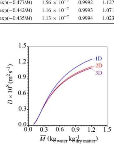
Figure6 presents the effective mass diffusivities as a function of the local moisture content for the cases one-(present work), two- [15] and three-dimensional [14].
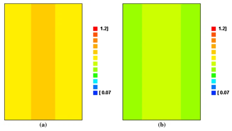
Figure7presents the moisture distributions for the one-dimensional case at instantst=19.8 h andt=31.2 h.
Discussion
According to several authors, such as Silva et al. [13], due to some heterogeneity and anisotropy, the diffusion process in a given direction can be little different from the diffusion in other directions. Thus, the values of the parameters
Fig. 2 Simplified flowchart for the optimization algorithm
highlight-ing the parameterh
Fig. 3 Parallelepiped representing a lumber with thicknessT, height
H and lengthL, highlighting the three moisture fluxes at the three visible surfaces during drying
determined by optimization should be interpreted as ef-fective values referring to the proposed model. In addition, Silva et al. [14] observe that the consideration of the liquid diffusion as the only mechanism of water transport inside the lumber is a simplification of the proposed model, jus-tified by the low value of the initial moisture content and drying temperature. Thus, the analyses in the following are performed in this context, i.e., considering the assumptions assumed for models 3D, 2D and 1D.
An inspection on the statistical indicators of Table1
enables to conclude that the drying kinetics of lumber was well described by three models used to represent the pro-cess. However, as Silva et al. [13] observed, the results of Table1indicates that the more the considered geometry is close to the real geometry, the better the results. On the other hand, an idea on the goodness-of-fit for the one-di-mensional case is given by inspection of Fig.5, in which the experimental points and the one-dimensional simula-tion are in good agreement. Similar result was obtained by Dincer [1], which used with success an analytical solution of the diffusion equation to describe drying of lumber with the following dimensions:T=40 mm, H=100 mm and
L=200 mm. Note that, in this case,HandLare 2.5 and 5 times the value of T, respectively. In the present study,
HandL are 2.8 and 20.7 times the value of T, and such dimensions are more favorable to consider the lumber as an infinite slab. In addition, Dincer [1] considered the effec-tive mass diffusivity with a constant value and in the pre-sent work, this property was considered variable. This
consideration is so significant that the statistical indicators obtained by Silva et al. [13] describing this same drying with an analytical three-dimensional solution (constant effective mass diffusivity) are worse than the statistical indicators obtained herein with a numerical one-dimen-sional solution (variable effective mass diffusivity).
As can be realized in Fig.6, the effective water diffu-sivity increases with increasing of the local moisture con-tent, and this result was also obtained by other researchers such as Silva et al. [5] studying osmotic dehydration of guava, and Olek and Weres [12] describing lumber drying. In addition, Fig.6 indicates that the effective mass diffu-sivity for model 2D is moderately greater than this property obtained with 3D model. On the other hand, the effective mass diffusivity for model 1D is significantly greater than this property for model 2D and, consequently, for model 3D. The interpretation of this result can be given with basis in Fig.3, which shows the dimensions of the lumber and the moisture fluxes at the three visible surfaces of the parallelepiped during drying. For the 3D case, the moisture flux occurs in three pairs of surfaces, involving the total area of 209840 mm2. For the 2D case, the pair of moisture fluxes at direction z was disregarded. Thus, the area in-volved in the moisture flux was 202640 mm2, representing about 97 % of the total area for the 3D case. For the 1D case, the pair of moisture fluxes at direction y was also disregarded. Consequently, with these considerations, the
Table 1 Results of the
optimization using models Model References D(m
2s-1) h(m s-1) R2
v2
1D Present work 1.87910-8exp(-0.477/M) 1.56910-7 0.9992 1.127910-3
2D Silva et al. [15] 1.61910-8exp(-0.442/M) 1.16910-7 0.9993 1.071910-3
3D Silva et al. [14] 1.57910-8exp(-0.435/M) 1.13910-7 0.9994 1.023910-3
Fig. 5 Drying kinetics of lumber using one-dimensional numerical
simulation
Fig. 6 Effective mass diffusivity as a function of the local moisture
moisture flux occurs in an area equal to 149000 mm2, which represents only about 71 % of the area for the 3D case. As it is observed, the great reduction in area when models 3D or 2D are substituted by model 1D explains the significant increasing in its effective mass diffusivity, as it can be seen in Fig.6. On the other hand, the small re-duction in area when model 3D is substituted by model 2D explains the little difference in their effective mass diffu-sivities. An inspection of Table1enables to conclude that similar results are also obtained for the convective mass transfer coefficients for the cases one-, two- and three-dimensional.
To determine the average value for the effective mass diffusivity, the following expression was used:
D¼
RM0
MeqDðMÞdM
RM0 MeqdM
ð13Þ
in which M0 and Meq are, respectively, the initial and
equilibrium moisture content. For the one-dimensional case, the average effective mass diffusivity was 8.7910-9m2s-1. This average value is compatible with the constant value obtained by several authors that use diffusion models in wood drying considering some resis-tance on the boundary, such as Dincer [1] (h=2.26910-7m s-1andD=3.24 910-9m2s-1).
An observation of Fig.7 indicates that the information on moisture distribution within the lumber is poor because the moisture distribution at direction z and, mainly, at di-rection y are not considered. Even so, if the main focus of the study is the drying kinetics, model 1D presents good results for lumber with the dimensions involved in this work. As Silva et al. [21] observed, even whether the proposed model is not completely acceptable in a given study, the one-dimensional numerical solution presented in
this article is useful because, through this solution, the obtained results serve as initial values for other optimiza-tion processes involving a model 3D (or 2D).
Finally, as observed by Silva et al. [15], the drying ki-netics of wood at low temperature was well described by models with an effective water diffusivity expressed by an exponential function, in which the exponent is proportional to the inverse of the local moisture content. However, this function was obtained for the specific dataset studied in this article, and more tests should be performed to know whe-ther good results are also obtained.
Conclusion
One-dimensional model considering variable effective mass diffusivity well describes the drying kinetics of the studied lumber. The obtained statistical indicators are comparable with those obtained for two- and three-di-mensional models.
The strong reduction in area of moisture flux of model 1D significantly overestimates the effective mass diffu-sivity and the convective mass transfer coefficient when compared with these properties obtained with model 3D (and also 2D). In addition, the moisture distribution is simplified to the one-dimensional case and, for that, such distribution is not appropriate to provide information for a subsequent study on stress and crack formation. However, the process parameters obtained in this study by mization serve, at least, as initial values for other opti-mization processes involving a model 3D.
Acknowledgments The first author would like to thank CNPq
(Conselho Nacional de Desenvolvimento Cientı´fico e Tecnolo´gico) for the support given to this research and for his research grant (Process Number 301697/2012-4).
Fig. 7 Moisture distributions
References
1. Dincer I (1998) Moisture transfer analysis during drying of slab woods. Heat Mass Transf 34:317–320
2. Da Silva WP, Silva CMDPS, Farias VSO, Silva DDPS (2010) Calculation of the convective heat transfer coefficient and cooling kinetics of an individual fig fruit. Heat Mass Transf 46:371–380 3. Da Silva WP, Silva CMDPS, Nascimento PL, Carmo JEF, Silva DDPS (2011) Influence of the geometry on the numerical simulation of the cooling kinetics of cucumbers. Spanish J Agric Res 9:242–251
4. Da Silva WP, Silva CMDPS, Lins MAA (2011) Determination of expressions for the thermal diffusivity of canned foodstuffs by the inverse method and numerical simulations of heat penetration. Int J Food Sci Technol 46:811–818
5. Silva WP, Aires JEF, Castro DS, Silva CMDPS, Gomes JP (2014) Numerical description of guava osmotic dehydration including shrinkage and variable effective mass diffusivity. LWT Food Sci Technol 59:859–866
6. Da Silva WP, Farias VSO, Neves GA, Lima AGB (2012) Modeling of water transport in roof tiles by removal of moisture at isothermal conditions. Heat Mass Transf 48:809–821 7. Baronas R, Ivanauskas F, Sapagovas M (1999) Modelling of
wood drying and an influence of lumber geometry on drying dynamics. Nonlinear Anal Model Control Vilnius IMI 4:11–22 8. Baronas R, Ivanauskas F, Juodeikiene I, Kajalavicius A (2001)
Modelling of moisture movement in wood during outdoor stor-age. Nonlinear Anal Model Control 6:3–14
9. Liu JY, Simpson WT, Verrill SP (2001) An inverse moisture diffusion algorithm for the determination of diffusion coefficient. Dry Technol 19:1555–1568
10. Kulasiri D, Woohead I (2005) On modelling the drying of porous materials: analytical solutions to coupled partial differential equations governing heat and moisture transfer. Math Probl Eng 2005:275–291
11. Ricardez AP, Sua´rez JR, Berumen LA (2005) The drying of red oak at vacuum pressure. Maderas Ciencia y Tecnologı´a 7:23–26 12. Olek W, Weres J (2007) Effects of the method of identification of the diffusion coefficient on accuracy of modeling bound water transfer in wood. Transp Porous Med 66:135–144
13. Silva WP, Silva LD, Silva CMDPS, Nascimento PL (2011) Op-timization and simulation of drying processes using diffusion models: application to wood drying using forced air at low temperature. Wood Sci Technol 45:787–800
14. Silva WP, Silva LD, Farias VSO, Silva CMDPS, Ataı´de JSP (2013) Three-dimensional numerical analysis of water transfer in wood: determination of an expression for the effective mass diffusivity. Wood Sci Technol 47:897–912
15. Silva WP, Silva CMDPS, Rodrigues AF (2014) Comparison between two- and three-dimensional diffusion models to describe wood drying at low temperature. Eur J Wood Prod 72:527–533 16. Patankar SV (1980) Numerical heat transfer and fluid flow.
Hemisphere Publishing Corporation, New York
17. Press WH, Teukolsky SA, Vetterling WT, Flannery BP (1996) Numerical recipes in fortran 77. The art of Scientific Computing, vol 2, 2nd edn. Cambridge University Press, New York, pp 1–933 18. Bevington PR, Robinson DK (1992) Data reduction and error analysis for the Physical Sciences, 2nd edn. WCB/McGraw-Hill, Boston
19. Taylor JR (1997) An introduction to error analysis, 2nd edn. University Science Books, Sausalito
20. Silva WP, Silva CMDPS, da Silva LD, Lins MAA (2012) Comparison between models with constant and variable diffu-sivity to describe water absorption by composite materials. Ma-terialwiss Werkstofftech 43:825–831