http://www.sciencepublishinggroup.com/j/cse doi: 10.11648/j.cse.20190302.11
On Delay-Range-Dependent and Delay-Rate-Dependent
Stability for Delayed Systems
Yuan He
1, Jintian Hu
1, Shuxia Wang
2, Liansheng Zhang
2, *1
Deparment of Automation, Beijing Institute of Petro-chemical Technology, Beijing, China 2
Deparment of Mathematics and Physics, Beijing Institute of Petro-chemical Technology, Beijing, China
Email address:
*
Corresponding author
To cite this article:
Yuan He, Jintian Hu, Shuxia Wang, Liansheng Zhang. On Delay-Range-Dependent and Delay-Rate-Dependent Stability for Delayed Systems. Control Science and Engineering. Vol. 3, No. 2, 2019, pp. 20-28. doi: 10.11648/j.cse.20190302.11
Received: September 27, 2019; Accepted: October 22, 2019; Published: October 28, 2019
Abstract:
It is well known that the phenomena of time delays are frequently encountered in many process and various control systems. The presence of delays can have an effect on system stability and performance, so ignoring them may lead to design flaws and incorrect analysis conclusions. Hence, the stability problem for time-delayed systems has received considerable attention in recent years. This brief focuses on the stability analysis for a class of delayed linear systems. Firstly, we construct a novel augmented Lyapunov-Krasovskii functional (LKF) which includes the lower, the upper bounds of the delay and the delay itself. Secondly, utilizing some integral inequalities and the reciprocally convex combination lemma, we obtain less conservative stability criteria formulated in form of linear matrix inequalities (LMIs). Finally, numerical examples are provided to show the effectiveness of the proposed method.Keywords:
Time Delay, Lyapunov-Krasovskii Functional (LKF), Linear Matrix Inequalities (LMIs)1. Introduction
Time delay universally emerges in various engineering systems such as networked control systems, aircraft, process control systems and long transmission lines in pneumatic systems. It is well known that time delay often leads to the oscillation, poor performance behavior even instability. Accordingly, many researchers have paid attention to the stability problems of delayed control systems over the past few decades.
To deduce stability sufficient conditions, a variety of methods were adopted, such as integral inequalities, the model transformation, the delay decomposition approach, the free-weighting matrices approach (FWMA) and the reciprocally convex lemmas (RCLs) and so on [1-32] and references therein. Recently, the FWMA, the Jensen’s or Wirtinger’s integral inequalities method and the RCLs are widely used.
In Wu et al [10], the FWMA was firstly developed to investigate the stability of delayed systems. Later, He et al. [12, 13] improved and extended this approach. Park and Ko [14] further generalized the FWMA to a new Lyapunov
functional. By contrast, the FWMA can keep a tradeoff between the conservatism and the computational complexity [12, 15-16]. However there is still some conservatism in such criteria and the criteria should be simplified.
conservatism of results based on integral inequalities and motivates our current work.
Recently, the convex combination method [17-20] and the RCLs [8, 23, 24, 27-29] have been introduced to discuss the stability of delayed systems. Shao [17] estimated the cross terms by using the convex combination rather than enlarging directly them as the lower and the upper bounds of the delay, respectively, and Ref. [18-20] followed this idea to cope with the stability of delayed systems. Park et al [23] presented a reciprocally convex combination lemma (RCCL), which can cope with the terms containing the delays just introducing a few slack matrices. Thus, the RCCL has become powerful tool to assess the integral terms with time-varying delays. Ref. [27-29] extended the RCCL, and developed some useful extended reciprocally convex matrix inequality to analyze the delayed control systems. However, there leaves some room to investigate further.
In this paper, a modified augmented LKF where more information about the delay includes is constructed. Some novel stability criteria are derived in terms of linear matrix inequalities (LMIs). At last, two examples are given to demonstrate the effectiveness of the proposed results.
Notations: Throughout the paper, the superscript “T” denotes the transpose of a matrix; n
ℝ and n m×
ℝ stand for the set of real vector with n-dimensional and real matrix of size n m× , respectively; P>0 (P≥0) symbolizes a symmetric positive definite (positive semi-definite) matrix;I
and 0 refer to the identity matrix and zero matrix with appropriate dimensions, respectively. Block diagonal matrix
is symbolized by diag{ }⋯ ;
1 2 1 2
{ , , , n} [ T, T, , T Tn]
col x x ⋯ x = x x ⋯ x . The symbol“*”denotes
the elements induced by symmetry in a symmetric matrix. In what follows, if not explicitly stated, matrices are assumed to have compatible dimensions.
2. Problem Formulation and
Preliminaries
Consider a linear delayed system:
2
( ) ( ) ( ( )), 0
( ) ( ), [ , 0]
d
x t Ax t A x t d t t
xθ ϕ θ θ h
= + − >
= ∈ −
ɺ
(1)
where ( )x t ∈ℝnis the state vector; nxn
A∈ℝ andAd∈ℝnxnare
system matrices; The initial condition
ϕ
( )t is a continuously differentiable vector-valued function;d t( )is a time-varying discrete delay and satisfies:1 2
0< ≤h d t( )≤h < +∞ (2)
( )
d tɺ ≤ < +∞µ (3)
whereh h1, 2andµare constants.
To begin with, we introduce the following lemmas which play an essential role in deriving our main results.
Lemma 1 (Jensen’s integral inequality [6]) For any real symmetric positive definite matrixM∈ n n×
ℝ , two scalars
α β
≤ and a vector-valued function ω( ) : [ , ]t α β →ℝnsuch that the following integration are well defined, then( ) β T( )t M ( )t dt β T( )t dt M β ( )t dt .
α α α
β α− ω ω ≥ ω ω
∫
∫
∫
(4)Lemma 2 (Jensen’s double integral inequality [18], [30]) For any real symmetric positive definite matrix n n
R∈ℝ × , two scalars satisfying
τ
2 > ≥τ
1 0, and a vector-valued functionω
( )t such that the following integration are well defined, then1 1 1
2 2 2
2 2
2 1 ( ) ( ) ( ) ( ) .
2
T
t t t
T
t t t
d s R s ds d s ds R d s ds
τ τ τ
τ λ τ λ τ λ
τ τ − λ ω ω − λ ω − λ ω
− + − + − +
−
≥
∫
∫
∫
∫
∫
∫
(5)3. Main Results
In this section, we are to discuss stability of system (1). For simplicity and convenience, we define
1
1 2
1 2 1 2
( )
( )
( ) { ( ), ( ( )), ( ), ( ), ( ), ( ), ( ) , ( ) , ( ) }
t t h t d t
t h t d t t h
t col x t x t d t x t h x t h x t h x t h x s ds x s ds x s ds
η
− −
− − −
= − − − − −
∫
∫
∫
ɺ ɺ
and
( 1) (9 )
[0 , , 0 ], 1, 2, ,9
T
i n i n n n i n
e = × − I × − i= ⋯ .
For system (1), we have main result as follows.
Theorem 1 For any givenh h1, 2andµ, the system (1) satisfying (2) and (3) is globally asymptotically stable if there
11 12 13 14 15
22 23 24 25
33 34 35
44 45
55 *
* * ,
* * *
* * * *
P P P P P
P P P P
P P P P
P P P
=
( 1, 2, 3, 4, 5), ( 1, 2, 3, 4)
i j
Q i= Z j= andR kk( =1, 2)such that for any matrices S1 and S2 the following LMIs hold simultaneously
2 1 2
0 *
Z S
Z
≥
,
4 2 4
0 *
Z S
Z
≥
(6)
2 2
1 1 1 3 12 4 1 2 3 2 3 2 1 3 3 4 2 4 5 5 4 5 6 5 6 7 3 7 8 4 8 8 2 9 9 4 9
3 2 2 3 2 3 2 1 2 4 2 4 2 2 4 1 1 7 1 1 1 7
( ) ( 1) ( )
( ) 2
( ) ( ) 2( ) ( ) ( ) ( )
( ) ( ) (
T T T T
T T T T T T T
T T T
T
e Q h Z h Z e e Q e e Q Q Q e
e Q e e Q Q e e Q e e Z e e Z e e S e e Z e
e e Z e e e e S e e e e Z e e
h e e R h e e h
µ
Ω + Γ ΥΓ + + + + − + − +
− + − − − − − −
− − − − − − − − −
− − − − 12 1 8 9) 2( 12 1 8 9) 0.
T
e − −e e R h e − −e e <
(7)
where
11 11 13 14 12 13 17 18 19 12 13 14 15 15 33 34 22 23 37 38 39
44 23 33 45 55 55 24 25 25 34 35 35
* 0 0 0
* *
* * *
* * * * 0 0
* * * * * 0
* * * * * * 0 0 0
* * * * * * * 0 0
* * * * * * * * 0
d
T T T T T
d d d d d
T T
P A P P
A P A P A P A P A P
P P
P P P P P
P P P
P P P
Ω Ω Ω Ω Ω Ω
Ω Ω Ω Ω Ω
Ω − − −
Ω =
11 11 11 14 14
T T
P A A P P P
Ω = + + + ,
13 15 14 12 24
T T
P P A P P
Ω = − + + ,
14 15 13 34
T T
P A P P
Ω = − + + ,
17 44 14
T
P A P
Ω = + ,
18 19 45 15
T
P A P
Ω = Ω = + ,
33 25 25 24 24
T T
P P P P
Ω = + − − ,
34 25 35 34
T T
P P P
Ω = − + − ,
37 45 44
T
P P
Ω = − ,
38 39 P55 P45
Ω = Ω = − ,
44 35 35
T
P P
Ω = − − ,
0 0 0 0 0 0 0
d
A A
Γ = ,
2 2 2 4
4 1 1 12 2 1 1 2
1
4 4
Q h Z h Z h R
γ
RΥ = + + + + ,
2 2 12 2 1, 2 1
h =h −h γ =h −h .
4
1
( )t i( )t
i
V x V x
=
=
∑
,where
1( )t
V x =ξT( )t Pξ( )t ,
1 1
1 2
2 1 2 3
( )
( )t t T( ) ( ) t h T( ) ( ) t h T( ) ( )
t h t h t d t
V x x
α
Q xα α
d − xα
Q xα α
d − xα
Q xα α
d− − −
=
∫
+∫
+∫
1
1 2
4 5
( ) ( ) ( ) ( )
t t h
T T
t hx
α
Q xα α
d t h xα
Q xα α
d−
− −
+
∫
ɺ ɺ +∫
ɺ ɺ ,1
1 2
0
3( ) 1 ( ) 1 ( ) 12 ( ) 2 ( )
t h t
T T
t
h t h t
V x d h x Z x d d h x Z x d
λ λ
λ
α
α α
−λ
α
α α
− + − +
=
∫
∫
ɺ ɺ +∫
∫
ɺ ɺ1 0
1 ( ) 3 ( )
t T
hd
θ
t θh xα
Z xα α
d− +
+
∫
∫
12
12 ( ) 4 ( )
h t T
h d
θ
t θh xα
Z xα α
d−
− +
+
∫
∫
,1
1 2
2 0 0 0
1
4( ) ( ) 1 ( ) ( ) 2 ( )
2 2
t h t
T T
t
h t h t
h
V x d d x s R x s ds d d x s R x s ds
θ α θ α
γ
θ α − θ α
− + − +
=
∫
∫
∫
ɺ ɺ +∫
∫
∫
ɺ ɺ ,with
1
1 2
1 2
( ) { ( ), ( ), ( ), ( ) , ( ) }
t t h
t h t h
t col x t x t h x t h x s ds x s ds
ξ
−− −
= − −
∫
∫
.Calculating the time derivative ofV x1( ),t V x2( ),t andV x3( )t respectively along the solution of the system (1) yields
1( ) 2 ( ) ( )
T t
V xɺ = ξ t Pξɺt =ηT( )t Ωη( )t (8)
whereΩis defined in Theorem 1.
2 1 1 2 1 3 1 2 2 2
3 4 1 5 4 1
2 5 2
( ) ( ) ( ) ( )( ) ( ) ( )( ) ( )
( 1) ( ( )) ( ( )) ( ) ( ) ( )( ) ( )
( )( ) ( )
T T T
t
T T T
T
V x x t Q x t x t h Q Q Q x t h x t h Q x t h x t d t Q x t d t x t Q x t x t h Q Q x t h x t h Q x t h
µ
≤ + − − + − + − − −
+ − − − + + − − −
+ − − −
ɺ
ɺ ɺ ɺ ɺ
ɺ ɺ
(9)
1
1 1
2 1 2
2 2 2 2
3 1 3 12 4 1 1 12 2 1 1
12 2 1 3 12 4
( ) ( )( ) ( ) ( )( ) ( ) ( ) ( )
( ) ( ) ( ) ( ) ( ) ( ) ,
t
T T T
t
t h
t h t t h
T T T
t h t h t h
V x x t h Z h Z x t x t h Z h Z x t h x Z x d
h x Z x d h x Z x d h x Z x d
−
− −
− − −
= + + + −
− − −
∫
∫
∫
∫
ɺ ɺ ɺ ɺ ɺ
ɺ ɺ
α α α
α α α α α α α α α (10)
Using Lemma 1 yields
1
1 ( ) 1 ( ) ( )(1 3) 1(1 3) ( )
t
T T T
t h
h x α Z xα αd η t e e Z e e η t
−
−
∫
ɺ ɺ ≤ − − − (11)and
1
1 ( ) 3 ( ) ( )7 3 7 ( )
t
T T T
t h
h x α Z xα αd η t e Z e η t
−
−
∫
≤ − (12)Observe that
1 1
2 2
( )
12 2 12 2 12 2
( )
( ) ( ) ( ) ( ) ( ) ( )
t h t d t t h
T T T
t h h x
α
Z xα α
d t h h xα
Z xα α
d t d t h xα
Z xα α
d− − −
− − −
Using Lemma 1 again, we have
2
( )
12 ( ) 2 ( )
t d t T
t h h x α Z xα αd
− − −
∫
ɺ ɺ 2 2 ( ) ( ) 2 1 2 2 ( ) ( ) ( ) Tt d t t d t
t h t h
h h
x d Z x d
h d t α α α α
− − − − − ≤ − −
∫
ɺ ∫
ɺ and 1 12 2 ( ) ( ) ( ) t h T t d th x α Z xα αd −
−
−
∫
ɺ ɺ 2 1 1 12 ( ) ( ) 1 ( ) ( ) ( ) T
t h t h
t d t t d t
h h
x d Z x d
d t h α α α α
− − − − − ≤ − −
∫
ɺ ∫
ɺ . Thus 1 2 2 2 1 1 12 2 ( ) ( ) 2 1 2 2 2 1 2 ( ) ( ) 1 ( ) ( ) ( ) ( ) ( ) ( ) ( ) . ( ) t h T t ht d t t d t
T
t h t h
t h t h
T
t d t t d t
h x Z x d h h
x d Z x d
h d t h h
x d Z x d
d t h
α α α α α α α α α α α − − − − − − − − − − − − ≤ − − − − −
∫
∫
∫
∫
∫
ɺ ɺ ɺ ɺ ɺ ɺFrom the reciprocally convex combination lemmas [23] and [27], there exists a matrixS1with appropriate dimension such that
2 1 2 0 * Z S Z ≥ then 1 1 2 2 1 1 2 2 ( ) ( )
2 1 2 1
2 2
( ) ( )
2 1
( ) 2 1 ( ) ( ) 2 ( ) ( ) ( ) ( ) ( ) ( ) ( ) ( ) * ( ) ( )
t d t t d t t h t h
T T
t h t h t d t t d t
T
t h t h
t d t t d t
t d t t d
t h t h
h h h h
x d Z x d x d Z x d
h d t d t h
x d x d
Z S
Z
x d x d
α α α α α α α α α α α α α α α α − − − − − − − − − − − − − − − − − − − − − − ≤ −
∫
∫
∫
∫
∫
∫
∫
ɺ ɺ ɺ ɺ ɺ ɺ ɺ ( )ɺ . t ∫
Namely 1 1 2 2 ( ) ( )2 1 2 1
2 2
( ) ( )
2 1
3 2 2 3 2 3 2 1 2 4 2 4 2 2 4
( ) ( ) ( ) ( )
( ) ( )
( )[( ) ( ) 2( ) ( ) ( ) ( ) ] ( ).
t d t t d t t h t h
T T
t h t h t d t t d t
T T T T
h h h h
x d Z x d x d Z x d
h d t d t h
t e e Z e e e e S e e e e Z e e t
α α α α α α α α η η − − − − − − − − − − − − − − ≤ − − − + − − + − −
∫
ɺ∫
ɺ∫
ɺ∫
ɺ (13)Similarly, there exists a matrixS2with appropriate dimension such that
4 2 4 0 * Z S Z ≥ , then 1 2
12 ( ) 4 ( ) ( )[ 8 4 8 28 2 9 9 4 9] ( )
t h
T T T T T
t h h x
α
Z xα α
dη
t e Z e e S e e Z eη
t− −
−
∫
≤ − + + (14)Additionally,
1
1 2
4 2 2 0
1 1
4( ) ( )( 1 2) ( ) ( ) 1 ( ) ( ) 2 ( )
4 4 2 2
t h t
T T T
t
h t h t
h h
V x x t R R x t d x s R x s ds d x s R x s ds
θ θ
γ θ γ − θ
− + − +
= + −
∫
∫
−∫
∫
ɺ ɺ ɺ ɺ ɺ ɺ ɺ (15)
1 2 0 1
1 1 1 7 1 1 1 7
( ) ( ) ( )[( ) ( ) ] ( )
2
t
T T T
h t
h
d x s R x s ds t h e e R h e e t
θ
θ η η
− +
−
∫
∫
ɺ ɺ ≤ − − − (16)and
1 2
2 12 1 8 9 2 12 1 8 9
( ) ( ) ( )[( ) ( ) ] ( ). 2
h t
T T T
h d t θx s R x s ds t h e e e R h e e e t
γ
−θ
η
η
− +
−
∫
∫
ɺ ɺ ≤ − − − − − (17)Combining with (8)-(17), one concludes
( )t T( ) ( ),
V xɺ ≤η t Ση t (18)
where
2 2
1 1 1 3 12 4 1 2 3 2 3 2 1 3 3 4 2 4 5 5 4 5 6 5 6 7 3 7 8 4 8 8 2 9 9 4 9
3 2 2 3 2 3 2 1 2 4 2 4 2 2 4 1 1 7 1 1 1 7
( ) ( 1) ( )
( ) 2
( ) ( ) 2( ) ( ) ( ) ( )
( ) ( )
T T T T
T T T T T T T
T T T
T
e Q h Z h Z e e Q e e Q Q Q e
e Q e e Q Q e e Q e e Z e e Z e e S e e Z e
e e Z e e e e S e e e e Z e e
h e e R h e e
µ
Σ = Ω + Γ ΥΓ + + + + − + − +
− + − − − − − −
− − − − − − − − −
− − − −( 12 1 8 9) 2( 12 1 8 9) .
T
h e − −e e R h e − −e e
According to the Lyapunov stability theory, if (6) and (7) hold, thenΣ <0, which ensure that system (1) is globally asymptotically stable. This completes the proof of Theorem 1.
Remark 1 In Ref. [3-4, 18], the cross term
1 2
2
( ) ( )
h t T
h d
θ
t θx s R x s ds−
− +
−
∫
∫
ɺ ɺarising in the derivative of V x( )t was enlarged directly by the Jensen’s double integral inequality. However, those
similar terms existing in the derivative of V x( )t such as
1 2
12 ( ) 4 ( )
t h T
t h h x s Z x s ds
− −
−
∫
, 12
12 ( ) 2 ( )
t h T
t h h x s Z x s ds
− −
−
∫
ɺ ɺ .For such integral terms, the authors of Ref. [3-4] and [18] firstly divided them into sum of two parts respectively. Each part was then enlarged by the Jensen’s integral inequality rather than being enlarged each term by directly the Jensen’s integral inequality. Specifically, that is
1 1
2 2
( )
12 4 12 4 12 4
( )
( ) ( ) ( ) ( ) ( ) ( )
t h t d t t h
T T T
t h t h t d t
h − x
α
Z xα α
d h − xα
Z xα α
d h − xα
Z xα α
d− − −
−
∫
= −∫
−∫
1 1
2 2
( ) ( )
12 12
4 4
( ) ( )
2 1
( ) ( ) ( ) ( )
( ) ( )
t d t t d t t h t h
T T
t h t h t d t t d t
h h
x s ds Z x s ds x s ds Z x s ds
h d t d t h
− − − −
− − − −
≤ − −
−
∫
∫
−∫
∫
not
1 1 1
2 2 2
12 ( ) 4 ( ) ( ) 4 ( )
t h t h t h
T T
t h t h t h
h − x s Z x s ds − x s Z − x s
− − −
−
∫
≤ −∫
∫
.Such approach can reduce conservatism in a way, as claimed in the literature, for example Ref. [17]. Therefore, it is unavoidable that such inconsistent tackle will lead to some conservatism. Differently from aforementioned previous literature,
we cope with the term 1
2
2
( ) ( )
h t T h t
d x s R x s ds
θ
θ
−
− +
−
∫
∫
ɺ ɺ as follows:1 1
2 2
( )
2 2 2
( )
( ) ( ) ( ) ( ) ( ) ( )
h t d t t h t
T T T
h d
θ
t θx s R x s ds h dθ
t θx s R x s ds d t dθ
t θx s R x s ds− − −
− + − + − +
−
∫
∫
ɺ ɺ = −∫
∫
ɺ ɺ −∫
∫
ɺ ɺ .Subsequently, we enlarge each part lying on the right-hand side of the above equality by Lemma 2. In short, we surmount the shortcoming iteming from such inconsistent tackle and obtain some less conservative conditions compared with those in the literature.
Remark 2 The conservatism reduction of the proposed
1 2
2
( ) ( )
t h T t h
x
α
Q xα α
d− −
∫
, 1 3( )
( ) ( )
t h T t d t
x α Q xα αd −
−
∫
, 12
12 ( ) 4 ( )
h t T h t
d h x Z x d
θ
θ
α
α α
−
− +
∫
∫
.Numerical examples are to validate such assertion further in section 4.
When the delay derivative may be unknown or does not exist, one can obtain a delay-dependent and delay-rate-independent stability criterion by setting Q3=0
in Theorem 1. That is:
Corollary 1 For givenh h1, 2, the system (1) subject to (2) is globally asymptotically stable if there exist symmetric
positive definite matrices with appropriate dimensions
5 5
[ ij] , i( 1, 2, 4, 5)
P= P × Q i= , Z ij( =1, 2, 3, 4)andR kk( =1, 2)
such that for any matricesS1andS2the following LMIs hold simultaneously
2 1 2
0 *
Z S
Z
≥
,
4 2 4
0 *
Z S
Z
≥
,
2 2
1 1 1 3 12 4 1 3 2 1 3 4 2 4 5 5 4 5 6 5 6 7 3 7 8 4 8 8 2 9 9 4 9
3 2 2 3 2 3 2 1 2 4 2 4 2 2 4 1 1 7 1 1 1 7 12 1 8 9 2 1
( ) ( )
( ) 2
( ) ( ) 2( ) ( ) ( ) ( )
( ) ( ) ( ) (
T T T T
T T T T T T
T T T
T
e Q h Z h Z e e Q Q e e Q e
e Q Q e e Q e e Z e e Z e e S e e Z e
e e Z e e e e S e e e e Z e e
h e e R h e e h e e e R h
Ω + Γ ΥΓ + + + + − −
+ − − − − − −
− − − − − − − − −
− − − − − − 2 1 8 9) 0.
T
e − −e e <
and notationsΩ Υ Γ, , are defined in Theorem 1.
4. Numerical Examples
In this section, two examples are presented to illustrate the proposed stability criteria in this paper.
Example 1. Consider the system (1) with
2.0 0.0
0.0 0.9
A=−
−
, 1
1.0 0.0
1.0 1.0
A =−
− −
.
For variousµand unknownµ, the allowable upper bound on delayh2, which ensures the globally asymptotic stability
of the system (1) for given lower boundh1are listed in Table 1 and Table 2, respectively. From Table 1, it is clear that the proposed method can give much largerh2than those in [3, 17, 18] in most of cases.
From Table 2, the proposed criterion is less conservative than those reported in [17-20] except the case whenh1=1.0.
Table 1. Allowable upper boundsh with different2 h and1 µfor Example 1. h1 Methods µ=0.30 µ=0.50 µ=0.90
2.0
[17] 2.6972 2.5048 2.5048
[18] 3.0129 2.5663 2.5663
[3] 3.0129 2.6099 2.6099
Theorem 1 3.0327 2.6137 2.6137
3.0
[17] 3.2591 3.2591 3.2591
[18] 3.3408 3.3408 3.3408
[3] 3.3891 3.3891 3.3891
Theorem 1 3.3912 3.3912 3.3912
4.0
[17] 4.0744 4.0744 4.0744
[18] 4.1690 4.1690 4.1690
[3] 4.1978 4.1978 4.1978
Theorem 1 4.1749 4.1749 4.1749
Table 2. Allowable upper boundsh with various2 h and unknown1 µfor Example 1.
Methods h1 1.0 2.0 3.0 4.0
[17] h2 1.8737 2.5049 3.2591 4.0744
[18] h2 1.9008 2.5663 3.3408 4.169
[19] h2 1.9422 2.5383 3.2749 4.0787
(N=1)
[20] h2 1.9422 2.5383 3.2749 4.0787
(N=1)
Corollary 1 h2 1.9127 2.5729 3.3517 4.1758
Example 2. Consider the system (1) with
0.0 1.0
1.0 2.0
A=
− −
, 1
0.0 0.0 1.0 1.0
A =
−
For variousµ and given lower boundh1, the allowable upper bound on delay h2, which guarantees the globally asymptotic stability of the system (1) is listed in Table 3. For
1 0
h = and variousµ, the allowable upper bound on delay
2
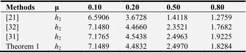
h , which ensures the globally asymptotic stability of the system (1) can be obtained in Table 4. From Tables 3 and 4, the proposed method in this paper gives largerh2 in most of cases than those in the literature.
Table 3. Allowable upper boundsh with various2 h and1 µ=0.3for Example 2.
Methods h1 0.30 0.50 0.80 1.0
[17] h2 2.2224 2.2278 2.2388 2.2474
[18] h2 2.2634 2.2858 2.3078 2.3167
Theorem 1 h2 2.2729 2.2932 2.3137 2.3228
Table 4. Allowable upper boundsh with various2 µandh1=0for Example 2. Methods µ 0.10 0.20 0.50 0.80
[21] h2 6.5906 3.6728 1.4118 1.2759
[32] h2 7.1480 4.4660 2.3521 1.7682
[31] h2 7.1765 4.5438 2.4963 1.9225
5. Conclusions
In this paper, we develop the delay-range-dependent stability criterion for delayed systems. The Jensen’s integral inequality, together with the reciprocally convex lemma, was employed and the derivative of the LKF was estimated more tightly. As a result, a novel stability criterion is derived and as by-product a delay-rate-independent criterion is also obtained. Two numerical examples are provided to substantiate the validity of the proposed method.
Although the proposed stability criteria do not remarkably have reduction in conservativeness, they are significant since there are fewer decisive variables including them and less computational complexity to test the proposed criteria.
Acknowledgements
The work is supported in part by the Science and Technology Plan of Beijing Municipal Education Commission under Grant KM201910017002.
References
[1] E. Fridman and U. Shaked. An improved stabilization method for linear time-delay systems. IEEE Transactions on Automatic Control, 2002; 47 (11): 1931-1937.
[2] J. Sun, G. P. Liu and J. Chen. Delay-dependent stability and stabilization of neutral time-delay systems. International Journal of Robust and Nonlinear Control, 2009; 19 (12): 1364-1375.
[3] O. M. Kwon, E. J. Cha. New stability criteria for linear system with interval time-varying state delay. Journal of Electrical Engineering & Technology, 2011; 6 (5): 713-722.
[4] T. Wang, A. G. Wu. Improved delay-range-dependent stability criteria for continuous linear system with time-varying delay. Proceedings of the 25th Chinese Control and Decision Conference, 2013; 182-187.
[5] J. H. Kim. Note on stability of linear systems with time-varying delay. Automatica, 2011; 47 (9): 2118-2121. [6] K. Gu, An integral inequality in the stability problem of
time-delay systems, Proceedings of 39th IEEE conference on decision and control, 2000; 2805-2810.
[7] Q. L. Han and K. Gu. Stability of linear systems with time-varying delay: a generalized discretized Lyapunov function approach. Asian Journal of Control, 2001; 13 (3): 170-180.
[8] W. Lee, P. Park. Second-order reciprocally convex approach to stability of systems with interval time-varying delays. Applied Mathematics and Computation, 2014; 229 (1): 245–253. [9] S. Xu and J. Lam. On equivalence and efficiency of certain
stability criteria for time-delay systems. IEEE Transactions on Automatic Control, 2007; 52 (1): 95-101.
[10] M. Wu, Y. He, J. H. She, and G. P. Liu. Delay-dependent criteria for robust stability of time-varying delay systems. Automatica, 2004; 40 (8): 1435-1439.
[11] P. L. Liu. Further improvement on delay-range-dependent stability results for linear systems with interval time-varying delays. ISA Trans, 2013; 52 (6): 725-729.
[12] Y. He, Q. G. Wang, L. Xie, and C. Lin. Further improvement of free-weighting matrices technique for systems with time-varying delay. IEEE Transactions on Automatic Control, 2007; 52 (2): 293-299.
[13] Y. He, Q. G. Wang, C. Lin, and M. Wu, Delay-range-dependent stability for systems with time-varying delay. Automatica, 2007; 43 (2): 371-376.
[14] P. Park and J. W. Ko. Stability and robust stability for systems with time-varying delay. Automatica, 2007; 43 (10): 1855-1858.
[15] X. Jiang and Q. L. Han. New stability criteria for linear systems with interval time-varying delay. Automatica, 2008; 44 (10): 2680-2685.
[16] X. Jiang, Q. L. Han, S. Liu, and A. Xue. A new H∞
stabilization criterion for networked control systems. IEEE Transactions on Automatic Control, 2008; 53 (4): 1025-1032. [17] H. Shao. New delay-dependent stability criteria for systems
with interval delay. Automatica, 2009; 45 (3): 744-749. [18] J. Sun, G. P. Liu, J. Chen, D. Rees. Improved
delay-range-dependent stability criteria for linear systems with time-varying delays. Automatica, 2010; 46 (2): 466-470. [19] X. L. Zhu, Y. Wang and G. H. Yang. New stability criteria for
continuous time systems with interval time-varying delay. IET Control Theory Appl., 2010; 4 (6): 1101-1107.
[20] M. Tang, Y. W. Wang and C. Y. Wen. Improved delay-range-dependent stability criteria for linear systems with interval time-varying delays. IET Control Theory Appl., 2012; 6 (6): 868-873.
[21] A. Seuret, F. Gouaisbaut. Wirtinger-based integral inequality: Application to time-delay systems. Automatica, 2013; 49 (9): 2860-2866.
[22] K. Liu, & E. Fridman, Wirtinger’s inequality and Lyapunov-based sampled-data stabilization. Automatica, 2012; 48 (1): 102-108.
[23] P. Park, W. Jeong, C. Jeong. Reciprocally convex approach to stability of systems with time-varying delays, Automatica, 2011; 47 (1): 235-238.
[24] J. An et al., A novel approach to delay-fractional-dependent stability criterion for linear systems with interval delay, ISA Trans., 2014; 53 (1): 210-219.
[25] J. H. Kim. Further improvement of Jensen inequality and application to stability of time-delayed systems. Automatica, 2016; 64 (1), 121-125.
[26] Éva Gyurkovics, A note on Wirtinger-type integral inequalities for time-delay systems, Automatica, 2015; 61 (1): 44-46. [27] A. Seuret, & F. Gouaisbaut, (2017). Delay-dependent
reciprocally convex combination lemma. http://hal.archives-ouvertes.fr/hal-01257670/.
[29] X. M. Zhang, Q. L. Han, A. Seuret, and F. Gouaisbaut, An improved reciprocally convex inequality and an augmented Lyapunov-Krasovskii functional for stability of linear systems with time-varying delay, Automatica, 2017; 84 (1): 221-226. [30] LS Zhang, L He, YD Song. New Results on Stability Analysis
of Delayed Systems Derived from Extended Wirtinger’s Integral Inequality, Neurocomputing, 2018; 283 (1): 98-106.
[31] T. H. Lee, J. H. Park, A novel Lyapunov functional for stability of time-varying delay systems via matrix-refined-function, Automatica, 2017; 80 (1): 239-247. [32] H.-B. Zeng, Y. He, M. Wu, & J. She. Free-matrix-based