University of Pennsylvania
ScholarlyCommons
Publicly Accessible Penn Dissertations
1-1-2013
Formalizing the SSA-based Compiler for Verified
Advanced Program Transformations
Jianzhou Zhao
University of Pennsylvania, [email protected]
Follow this and additional works at:
http://repository.upenn.edu/edissertations
Part of the
Computer Sciences Commons
This paper is posted at ScholarlyCommons.http://repository.upenn.edu/edissertations/825 For more information, please [email protected].
Recommended Citation
Zhao, Jianzhou, "Formalizing the SSA-based Compiler for Verified Advanced Program Transformations" (2013).Publicly Accessible Penn Dissertations. 825.
Formalizing the SSA-based Compiler for Verified Advanced Program
Transformations
Abstract
Compilers are not always correct due to the complexity of language semantics and transformation algorithms, the trade-offs between compilation speed and verifiability,etc.The bugs of compilers can undermine the source-level verification efforts (such as type systems, static analysis, and formal proofs) and produce target programs with different meaning from source programs. Researchers have used mechanized proof tools to implement verified compilers that are guaranteed to preserve program semantics and proved to be more robust than ad-hoc non-verified compilers.
The goal of the dissertation is to make a step towards verifying an industrial strength modern compiler--LLVM, which has a typed, SSA-based, and general-purpose intermediate representation, therefore allowing more advanced program transformations than existing approaches. The dissertation formally defines the sequential semantics of the LLVM intermediate representation with its type system, SSA properties, memory model, and operational semantics. To design and reason about program transformations in the LLVM IR, we provide tools for interacting with the LLVM infrastructure and metatheory for SSA properties, memory safety, dynamic semantics, and control-flow-graphs. Based on the tools and metatheory, the dissertation implements verified and extractable applications for LLVM that include an interpreter for the LLVM IR, a transformation for enforcing memory safety, translation validators for local optimizations, and verified SSA construction transformation.
This dissertation shows that formal models of SSA-based compiler intermediate representations can be used to verify low-level program transformations, thereby enabling the construction of high-assurance compiler passes.
Degree Type
Dissertation
Degree Name
Doctor of Philosophy (PhD)
Graduate Group
Computer and Information Science
First Advisor
Steve Zdancewic
Subject Categories
FORMALIZING THE SSA-BASED COMPILER FOR VERIFIED
ADVANCED PROGRAM TRANSFORMATIONS
Jianzhou Zhao
A DISSERTATION
in
Computer and Information Science
Presented to the Faculties of the University of Pennsylvania
in
Partial Fulfillment of the Requirements for the
Degree of Doctor of Philosophy
2013
Steve Zdancewic, Associate Professor of Computer and Information Science Supervisor of Dissertation
Val Tannen, Professor of Computer and Information Science Graduate Group Chairperson
Dissertation Committee
Andrew W. Appel, Eugene Higgins Professor of Computer Science
Milo M. K. Martin, Associate Professor of Computer and Information Science
Benjamin Pierce, Professor of Computer and Information Science
ABSTRACT
FORMALIZING THE SSA-BASED COMPILER FOR VERIFIED ADVANCED PROGRAM
TRANSFORMATIONS
Jianzhou Zhao
Steve Zdancewic
Compilers are not always correct due to the complexity of language semantics and
transfor-mation algorithms, the trade-offs between compilation speed and verifiability, etc. The bugs of
compilers can undermine the source-level verification efforts (such as type systems, static analysis,
and formal proofs) and produce target programs with different meaning from source programs.
Re-searchers have used mechanized proof tools to implement verified compilers that are guaranteed to
preserve program semantics and proved to be more robust than ad-hoc non-verified compilers.
The goal of the dissertation is to make a step towards verifying an industrial strength modern
compiler—LLVM, which has a typed, SSA-based, and general-purpose intermediate representation,
therefore allowing more advanced program transformations than existing approaches. The
disser-tation formally defines the sequential semantics of the LLVM intermediate represendisser-tation with its
type system, SSA properties, memory model, and operational semantics. To design and reason
about program transformations in the LLVM IR, we provide tools for interacting with the LLVM
infrastructure and metatheory for SSA properties, memory safety, dynamic semantics, and
control-flow-graphs. Based on the tools and metatheory, the dissertation implements verified and extractable
applications for LLVM that include an interpreter for the LLVM IR, a transformation for
enforc-ing memory safety, translation validators for local optimizations, and verified SSA construction
transformation.
This dissertation shows that formal models of SSA-based compiler intermediate representations
can be used to verify low-level program transformations, thereby enabling the construction of
Contents
1 Introduction 1
2 Background 5
2.1 Program Refinement . . . 5
2.2 Static Single Assignment . . . 7
2.3 LLVM . . . 9
2.4 The Simple SSA Language—Vminus . . . 10
3 Mechanized Verification of Computing Dominators 12 3.1 The Specification of Computing Dominators . . . 13
3.1.1 Dominance . . . 13
3.1.2 Specification . . . 15
3.1.3 Instantiations . . . 16
3.2 The Allen-Cocke Algorithm . . . 17
3.2.1 DFS: PO-numbering . . . 18
3.2.2 Kildall’s algorithm . . . 21
3.2.3 The AC algorithm . . . 23
3.3 Extension: the Cooper-Harvey-Kennedy Algorithm . . . 25
3.3.1 Correctness . . . 25
3.4 Constructing Dominator Trees . . . 27
3.5 Dominance Frontier . . . 28
3.6 Performance Evaluation . . . 29
4.1 Dynamic Semantics . . . 32
4.2 Dominance Analysis . . . 34
4.3 Static Semantics . . . 35
5 Proof Techniques for SSA 37 5.1 Safety of Vminus . . . 38
5.2 Generalizing Safety to Other SSA Invariants . . . 39
5.3 The Correctness of SSA-based Transformations . . . 40
6 The formalism of the LLVM IR 43 6.1 The Syntax . . . 43
6.2 The Static Semantics . . . 48
6.3 A Memory Model for the LLVM IR . . . 49
6.3.1 Rationale . . . 49
6.3.2 LLVM memory commands . . . 50
6.3.3 The byte-oriented representation . . . 52
6.3.4 The LLVM flattened values and memory accesses . . . 53
6.4 Operational Semantics . . . 54
6.4.1 Nondeterminism in the LLVM operational semantics . . . 55
6.4.2 Nondeterministic operational semantics of the SSA form . . . 58
6.4.3 Partiality, preservation, and progress . . . 58
6.4.4 Deterministic refinements . . . 60
6.5 Extracting an Interpreter . . . 62
7 Verified SoftBound 64 7.1 Formalizing SoftBound for the LLVM IR . . . 65
7.2 Extracted Verified Implementation of SoftBound . . . 70
8 Verified SSA Construction for LLVM 73 8.1 Themem2regOptimization Pass . . . 73
8.2 Thevmem2regAlgorithm . . . 79
8.3.1 Preserving promotability . . . 84
8.3.2 Preserving well-formedness . . . 85
8.3.3 Program refinement . . . 87
8.3.4 The correctness ofvmem2reg . . . 91
8.4 Extraction and Performance Evaluation . . . 91
8.5 Optimizedvmem2reg . . . 93
8.5.1 O1 Level—Pipeline fusion . . . 94
8.5.2 The Correctness ofvmem2reg-O1 . . . 98
8.5.3 O2 Level—Minimalφ-nodes Placement . . . 105
8.5.4 The Correctness ofvmem2reg-O2 . . . 107
9 The Coq Development 111 9.1 Definitions . . . 111
9.2 Proofs . . . 112
9.3 OCaml Bindings and Coq Extraction . . . 113
10 Related Work 114
11 Conclusions and Future Work 118
List of Tables
3.1 Worst-case behavior. . . 30
List of Figures
2.1 Simulation diagrams that imply program refinement. . . 7
2.2 An SSA-based optimization. . . 8
2.3 The LLVM compiler infrastructure . . . 9
2.4 Syntax of Vminus . . . 10
3.1 The specification of algorithms that find dominators. . . 15
3.2 Algorithms of computing dominators . . . 16
3.3 The postorder (left) and the DFS execution sequence (right). . . 17
3.4 The DFS algorithm. . . 18
3.5 Termination of the DFS algorithm. . . 19
3.6 Inductive principle of the DFS algorithm. . . 21
3.7 Kildall’s algorithm. . . 22
3.8 The dominator trees (left) and the execution of CHK (right). . . 26
3.9 The definition and well-formedness of dominator trees. . . 27
3.10 Analysis overhead over LLVM’s dominance analysis for our extracted analysis. . . 29
4.1 Operational Semantics of Vminus (excerpt) . . . 33
4.2 Static Semantics of Vminus (excerpt) . . . 36
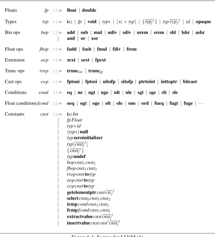
6.1 Syntax for LLVM (1). . . 44
6.2 Syntax for LLVM (2). . . 45
6.3 An example use of LLVM’s memory operations. . . 46
6.4 Vellvm’s byte-oriented memory model. . . 51
6.6 LLVMND: Small-step, nondeterministic semantics of the LLVM IR (selected rules). . . 56
7.1 SBspec: The specification semantics for SoftBound. Differences from the LLVMND rules are highlighted. . . 66
7.2 Simulation relations of the SoftBound pass . . . 69
7.3 Execution time overhead of the extracted and the C++ version of SoftBound . . . 71
8.1 The tool chain of the LLVM compiler . . . 74
8.2 Normalized execution time improvement of the LLVM’s mem2reg, LLVM’s O1, and LLVM’s O3 optimizations over the LLVM baseline with optimizations disabled. For comparison, GCC-O3’s speedup over the same baseline is also shown. . . 75
8.3 The algorithm ofmem2reg . . . 76
8.4 The SSA construction by themem2regpass . . . 77
8.5 The SSA construction by thevmem2regpass . . . 80
8.6 Basic structure ofvmem2reg_fn . . . 81
8.7 The algorithm ofvmem2reg . . . 82
8.8 The simulation relation for the correctness ofφ-node placement . . . 88
8.9 The simulation relation forDSEandDAE . . . 90
8.10 Execution speedup over LLVM-O0for both the extractedvmem2regand the original mem2reg. . . 92
8.11 Compilation overhead over LLVM’s originalmem2reg. . . 93
8.12 Basic structure ofvmem2reg-O1 . . . 94
8.13 eliminate stldofvmem2reg-O1 . . . 95
8.14 The operations for elimination actions . . . 96
8.15 Basic structure ofvmem2reg-O2 . . . 97
8.16 eliminate stldofvmem2reg-O2 . . . 106
8.17 The algorithm of insertingφ-nodes . . . 107
11.1 The effectiveness of GVN . . . 119
List of Abbreviations
AC Allen-Cocke.
ADCE Aggressive dead code elimination.
AH Aycock and Horspool.
CFG Control-flow graph.
CHK Cooper-Harvey-Kennedy.
DAE Dead alloca elimination.
DFS Depth first search.
DSE Dead store elimination.
GVN Global value numbering.
IR Intermediate representation.
LAA Load after alloca.
LAS Load after store.
LICM Loop invariant code motion.
LT Lengauer-Tarjan.
PO Postorder.
PRE Partial redundancy elimination.
SAS Store after store.
SCCP Sparse conditional constant propagation.
Chapter 1
Introduction
Compiler bugs can manifest as crashes during compilation or even result in the silent generation of
incorrect program binaries. Such mis-compilations can introduce subtle errors that are difficult to
diagnose and generally puzzling to the software developers. A recent study [73] used random
test-case generation to expose serious bugs in mainstream compilers including GCC [2], LLVM [38],
and commercial tools. Whereas few bugs were found in the front end of the compiler, various
optimization phases of the compiler that aim to make the generated program faster was a prominent
source of bugs.
Improving the correctness of compilers is a worthy goal. Large-scale source-code verification
efforts (such as the seL4 OS kernel [36] and Airbus’s verification of fly-by-wire software [61]),
gram invariants checked by sophisticated type systems (such as Haskell and OCaml), and sound
pro-gram synthesis (for example, Matlab/Simulink parallelizes high-level languages into C to achieve
high performance [3]) can be undermined by an incorrect compiler. The need for correct compilers
is amplified when compilers are parts of the trusted computing base in modern computer systems
that include mission-critical financial servers, life-critical pacemaker firmware, and operating
sys-tems.
Verified Compilers are tackling the problem of compiler bugs by giving a rigorous proof that a
compiler preserves the behavior of programs. The CompCert project [42, 68, 69, 70] first
imple-mented a realistic and mechanically verified compiler that is programmed andmechanically verified
in the Coq proof assistant [25] and generates compact and efficient assembly code for a large
Whereas the study uncovered many bugs in other compilers, the only bugs found in CompCert were
in those parts of the compiler not formally verified:
“The apparent unbreakability of CompCert supports a strong argument that developing compiler optimizations within a proof framework, where safety checks are explicit and machine-checked, has tangible benefits for compiler users.”
Despite CompCert’s groundbreaking compiler-verification efforts, there still remain many
chal-lenges in applying its technology to industrial-strength compilers. In particular, the original
Comp-Cert development and the bulk of the subsequent work—with the notable exception of CompComp-Cert-
CompCert-SSA [14] (which is concurrent with our work)—did not use astatic single assignment (SSA)[28]
intermediate representation (IR), as Leroy [42] explains:
“Since the beginning of CompCert we have been considering using SSA-based inter-mediate languages, but were held off by two difficulties. First, the dynamic semantics for SSA is not obvious to formalize. Second, the SSA property is global to the code of a whole function and not straightforward to exploit locally within proofs.”
In SSA, each variable is assigned statically only once and each variable definition must
dom-inate all of its uses in the control-flow graph. These SSA properties simplify or enable many
compiler optimizations [49, 71] including: sparse conditional constant propagation (SCCP),
ag-gressive dead code elimination (ADCE), global value numbering (GVN), common subexpression
elimination (CSE), global code motion, partial redundancy elimination (PRE), inductive variable
analysis (indvars) andetc.Consequently, open-source and commercial compilers such as GCC [2],
LLVM [38], Java HotSpot JIT [57], Soot framework [58], and Intel CC [59] use SSA-based IRs.
Despite their importance, there are few mechanized formalizations of the correctness properties
of SSA transformations. This dissertation tackles this problem by developing formal semantics
and proof techniques suitable for mechanically verifying the correctness of SSA-based compilers.
We do so in the context of our Vellvm framework, which formalizes the operational semantics of
programs expressed in LLVM’s SSA-based IR [43] and provides Coq [25] infrastructure to facilitate
mechanized proofs of properties about transformations on the LLVM IR. Moreover, because the
LLVM IR is expressive to represent arbitrary program constructors, maintain properties from
high-level programs, and hide details about target platforms, we define Vellvm’s memory model to
encode data along with high-level type information and to support arbitrary bit-width integers,
The Vellvm infrastructure, along with Coq’s facility for extracting executable code from
con-structive proofs, enables Vellvm users to manipulate LLVM IR code with high confidence in the
results. For example, using this framework, we can extract verified LLVM transformations that
plug directly into the LLVM compiler. In summary,
Thesis statement:Formal models of SSA-based compiler intermediate representations can be used to verify low-level program transformations, thereby enabling the construction of high-assurance compiler passes.
Contributions The specific contributions of the dissertation include:
• The dissertation formally defines the sequential semantics of the industrial strength
mod-ern compiler intermediate representation—the LLVM IR that includes its type system, SSA
properties, memory model, and operational semantics.
• To design and reason about program transformations in the IR, the dissertation designs tools
for interacting with the LLVM infrastructure, and metatheory for SSA properties, memory
safety, dynamic semantics, and control-flow-graphs.
• Based on the tools and metatheory, we implement verified and extractable applications for
LLVM that include the interpreter of the LLVM IR, a transformation for enforcing memory
safety, translation validators for local optimizations, and SSA construction.
The dissertation is based on our published work [75, 76, 77]. The rest of the dissertation is
organized as follows: Chapter 2 presents the background and preliminaries used in the dissertation.
To streamline the formalization of the SSA-based transformations, Chapter 2 also describes
Vmi-nus, a simpler subset of our full LLVM formalization—Vellvm [75], but one that still captures the
essence of SSA. Chapter 3 formalizes one crucial component of SSA-based compilers—computing
dominators [77]. Chapter 4 shows the dynamic and static semantics of Vminus. Chapter 5 describes
the proof techniques we have developed for formalizing properties of SSA-style intermediate
repre-sentations in the context of Vminus [76]. To demonstrate that our proof techniques can be used for
practical compiler optimizations, Chapter 6 shows the syntax of the full LLVM IR—Vellvm. Then,
Chapter 6 formalizes the semantics of Vellvm. Chapter 7 presents an application of Vellvm—a
veri-fied program transformation that hardens C programs against spatial memory safety violations (e.g.,
our proof techniques developed in Chapter 5 can be used for practical compiler optimizations in
Vel-lvm: verifying the most performance-critical optimization pass in LLVM’s compilation strategy—
themem2regpass [76]. Chapter 9 summarizes our Coq development. Finally, Chapter 10 discusses
Chapter 2
Background
This chapter presents the background and preliminaries used in the dissertation.
2.1
Program Refinement
In this dissertation, we prove the correctness of a compiler by showing that its output programP0
preserves the semantics of its original programP: informally,P0cannot do more than whatPdoes, although P0 can have fewer behaviors thanP. With this correctness, a compiler ensures that the analysis and verification results for source programs still hold after compilation.
Formally, we use program refinement to formalize semantic preservation. Following the
Comp-Cert project [42], we define program refinement in terms of programs’ external behaviors (which
include program traces of input-output events, whether a program terminates, and the returned value
if a program terminates): a transformed programrefinesthe original if the behaviors of the original
program include all the behaviors of the transformed program. We define the operational semantics
using traces of a labeled transition system.
Events e : := v=fid(vjj)
Finite traces t : := ε | e,t
Finite or infinite traces T : := ε | e,T (coinductive)
We denote one small-step of evaluation asconfig`S−→t S0: in program environmentconfig, pro-gram stateStransitions to the stateS0, recording eventseof the transition in the tracet. An evente
the reflexive, transitive closure of the small-step evaluation with a finite tracet. config`S−→T ∞
denotes a diverging evaluation starting fromSwith a finite or infinite traceT. Program refinement
is given by the following definition.
Definition 1(Program refinement).
1. init(prog,fid,vjj,S)means S is the initial program state of the program prog with the main
entry fid and inputs vj.
2. final(S,v)means S is the final state with the return value v.
3. ⇐(prog,fid,vjj,t,v)means∃S S0.init(prog,fid,vjj,S), config`S t ∗
−→S0andfinal(S0,v). 4. ⇒(prog,fid,vjj,T)means∃S.init(prog,fid,vjj,S)and config`S
T −→∞.
5. 6⇐(prog,fid,vjj,t)means∃S S0.init(prog,fid,vjj,S), config`S t ∗
−→S0and S0is stuck.
6. defined(prog,fid,vjj)means∀t,¬ 6⇐(prog,fid,vjj,t)
7. prog2refinesprogram prog1, written prog1⊇prog2, if
(a) defined(prog1,fid,vjj)
(b) ⇐(prog2,fid,vjj,t,v) ⇒ ⇐(prog1,fid,vjj,t,v)
(c) ⇒(prog2,fid,vjj,T) ⇒ ⇒(prog1,fid,vjj,T)
(d) 6⇐(prog2,fid,vjj,t) ⇒ 6⇐(prog1,fid,vjj,t)
Note that refinement requires only that a transformed program preserves the semantics of a
well-defined original program, but does not constrain the transformation of undefined programs.
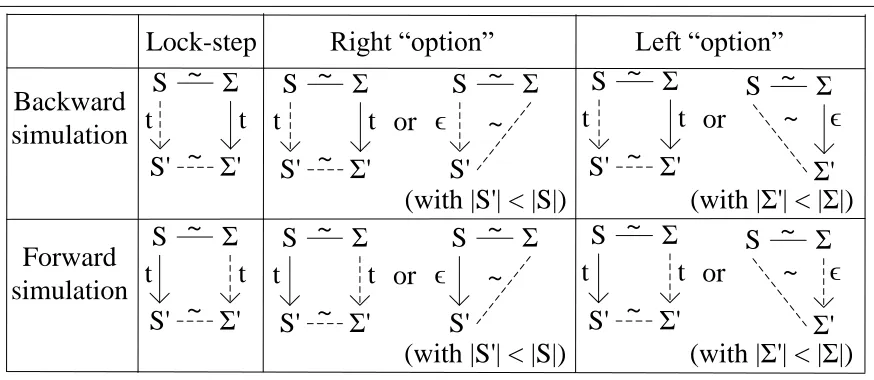
We use the simulation diagrams in Figure 2.1 to prove that a program transformation satisfies
the refinement property. Note that in Figure 2.1, we use S to denote program states of a source
program and useΣto denote program states of a target program. The backward simulation diagrams
imply program refinement for both deterministic and non-deterministic semantics. The forward
simulation diagrams (which are similar to the diagrams the CompCert project [42] uses) imply
program refinement for deterministic semantics. In each diagram, the program states of original
and compiled programs are on the left and right respectively. A line denotes a relation∼between
Σ
Lock-step
S
Σ'
S'
t
t
~
~
Σ
S
Σ'
ϵ
~
~
Σ
S
S'
ϵ
~
~
Σ
S
Σ'
S'
t
t
~
~
Right “option”
or
Σ
S
Σ'
S'
t
t
~
~
Left “option”
or
(with |S'| < |S|)
(with |Σ'| < |Σ|)
Σ
S
Σ'
S'
t
t
~
~
Σ
S
Σ'
ϵ
~
~
Σ
S
S'
ϵ
~
~
Σ
S
Σ'
S'
t
t
~
~
or
Σ
S
Σ'
S'
t
t
~
~
or
(with |S'| < |S|)
(with |Σ'| < |Σ|)
Backward
simulation
Forward
simulation
Figure 2.1: Simulation diagrams that imply program refinement.
At a high-level, we first need to find a relation∼between program states and their transformed
counterparts. The relation must hold initially, imply equivalent returned values finally, and imply
that stuck states are related. Then, depending on the transformation, we prove that a specific
diagram holds: lock-step simulation is for variable substitution, right “option” simulation is for
instruction removal, and left “option” simulation is for instruction insertion. Because the existence
of a diagram implies that the source and target programs share traces, we can prove the equivalence
of program traces by decomposing program transitions into matched diagrams. To ensure that an
original program terminates iff the transformed program terminates, the “option” simulations are
parameterized by a measure of program states|S|that must decrease to prevent “infinite stuttering”
problems.
2.2
Static Single Assignment
One of the crucial analysis in compiler design is determining values of temporary variables
stati-cally. With the analysis, compilers can reason about equivalence among variables and expressions,
and then eliminate redundant computation to reduce the runtime overhead. However, the analysis
for an ordinary imperative language is not trivial: a temporary variable can be defined more than
once; therefore, at runtime its value introduced at one definition is alive only by the next definition
of the variable. Moreover, because program transformations can add or remove temporary variables,
Original Transformed
l1:· · · · · · brr0l2l3
l2:r3=phi int[0,l1][r5,l2]
r4:=r1∗r2
r5:=r3+r4
r6:=r5 ≥100
brr6l2l3
l3:r7=phi int[0,l1][r5,l2]
r8:=r1∗r2
r9:=r8+r7
l1:· · ·
r4:=r1∗r2 brr0l2l3
l2:r3=phi int[0,l1][r5,l2]
r5:=r3+r4
r6:=r5 ≥100
brr6l2l3
l3:r7=phi int[0,l1][r5,l2]
r9:=r4+r7
In the original program (left),r1∗r2 is a partial common expression for the definitions of r4 and
r8, because there is no domination relation betweenr4andr8. Therefore, eliminating the common expression directly is not correct. For example, we cannot simply replacer8:=r1∗r2 byr8:=r4 sincer4 is not available at the definition ofr8 if the blockl2 does not execute before l3 runs. To transform this program, we might first move the instructionr4:=r1∗r2 from the block l2 to the blockl1 because the definitions ofr1andr2 must dominatel1, andl1 dominatesl2. Then we can safely replace all the uses ofr8byr4, because the definition ofr4inl1 dominatesl3and therefore dominates all the uses ofr8. Finally,r8is removed, because there are no uses ofr8.
Figure 2.2: An SSA-based optimization.
To address the issue, Static Single Assignment (SSA) form [28]1 was proposed to enforce
referential transparency syntactically [9], therefore simplifying program analysis for compilers.
Informally, SSA form is an intermediate representation distinguished by its treatment of temporary
variables—each such variable may be defined only once, statically, and each use of the variable must
be dominated by its definition with respect to the control-flow graph of the containing function.
Informally, the variable definition dominates a use if all possible execution paths to the use go
through the definition first.
To maintain these invariants in the presence of branches and loops, SSA form uses φ
-instructions, which act like control-flow dependent move operations. Suchφ-instructions appear
only at the start of a basic block and, crucially, they are handled specially in the dominance relation
to “cut” apparently cyclic data dependencies.
1In the literature, there are different variants of SSA forms [16]. We use the LLVM SSA form: for example, memory
C, C++, Haskell,
ObjC, ObjC++,
Scheme, Scala...
Alpha, ARM,
PowerPC, Sparc,
X86, Mips,
…
Code
Generator/
JIT
LLVM IR
Optimizations/
Transformations
Program analysis
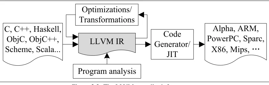
Figure 2.3: The LLVM compiler infrastructure
The left part of Figure 2.2 shows an example program in SSA form, written using the
stripped-down notation of Vminus (defined more formally in Section 2.4). The temporaryr3at the beginning
of the block labeledl2 is defined by aφ-instruction: if control enters the blockl2by jumping from
basic blockl1,r3will get the value 0; if control enters from blockl2(via the back edge of the branch
at the end of the block), thenr3will get the value ofr5.
The SSA form is good for implementing optimizations because it identifies variable names with
the program points at which they are defined. Maintaining the SSA invariants thus makes definition
and use information of each variable more explicit. Also, because each variable is defined only
once, there is less mutable state to be considered (for purposes of aliasing,etc.) in SSA form, which
makes certain code transformations easier to implement.
Program transformations like the one in Figure 2.2 are correct if the transformed program refines
the original program (in the sense described above) and the result is well-formed SSA. Proving
that such code transformations are correct is nontrivial because they involve non-local reasoning
about the program. Chapter 5 describes how such optimizations can be formally proven correct by
breaking them into micro transformations, each of which can be shown to preserve the semantics of
the program and maintain the SSA invariants.
2.3
LLVM
LLVM [43] (Low-Level Virtual Machine) is a robust, industrial-strength, and open-source
compi-lation framework. LLVM uses a typed, platform-independent SSA-based IR originally developed
Types typ : := int Constants cnst : := Int
Values val : := r | cnst
Binops bop : := + | ∗ | && |=| ≥ | ≤ | · · · Right-hand-sides rhs : := val1bop val2
Commands c : := r:=rhs
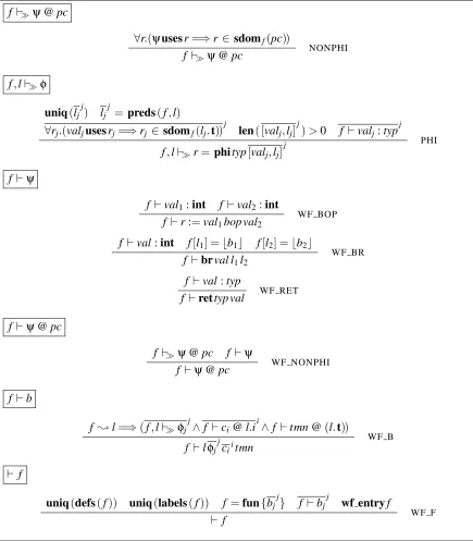
Terminators tmn : := brval l1l2 | rettyp val Phi Nodes φ : := r= phityp[valj,lj]
j
Instructions insn : := φ | c | tmn
Non-φs ψ : := c | tmn
Blocks b : := lφctmn
Functions f : := fun{b}
Figure 2.4: Syntax of Vminus
that competes with GCC in terms of compilation speed and performance of the generated code [38].
As a consequence, it has been widely used in both academia and industry2.
An LLVM-based compiler is structured as a translation from a high-level source language to the
LLVM IR (see Figure 2.3). The LLVM tools provide a suite of IR to IR translations, which provide
optimizations, program transformations, and static analyses. The resulting LLVM IR code can then
be lowered to a variety of target architectures, including x86, PowerPC, and ARM (either by static
compilation or dynamic JIT-compilation). The LLVM project focuses on C and C++ front-ends, but
many source languages, including Haskell, Scheme, Scala, Objective C and others have been ported
to target the LLVM IR.
2.4
The Simple SSA Language—Vminus
To streamline the formalization of the SSA-based transformations, we describe the properties
and proof techniques of SSA in the context of Vminus, a simpler subset of our full LLVM
formalization—Vellvm [75], but one that still captures the essence of SSA.
Figure 2.4 gives the syntax of Vminus. Every Vminus expression is of type integer. Operations
in Vminus compute with valuesval, which are either identifiersrnaming temporaries or constants
cnstthat must be integer values. We useRto range over sets of identifiers.
All code in Vminus resides in a top-level function, whose body is composed of blocksb. Here,
bdenotes a list of blocks; we also use similar notation for other lists. As is standard, a basic block
consists of a labeled entry pointl, a series of φ nodes, a list of commands cs, and a terminator
instructiontmn. In the following, we also use the labellof a block to denote the block itself.
Because SSA ensures the uniqueness of variables in a function, we use r to identify
instruc-tions that assign temporaries. For instrucinstruc-tions that do not update temporaries, such as terminators,
we introduce “ghost” identifiers to identify them—r: brval l1l2. Ghost identifiers satisfy
unique-ness statically but do not have dynamic semantics, and are not shown when we do not distinguish
instructions.
The set of blocks making up the top-level function constitutes a control-flow graph with a
well-defined entry point that cannot be reached from other blocks. We write f[l] =bbcif there is a block
bwith labellin function f. Here, theb c(pronounced “some”) indicates that the function is partial
(might return “none” instead).
As usual in SSA, the φ nodes join together values from a list of predecessor blocks of the
control-flow graph—eachφnode takes a list of (value, label) pairs that indicates the value chosen
when control transfers from a predecessor block with the associated label. The commandscinclude
the usual suite of binary arithmetic or comparison operations (bop—e.g.,addition+, multiplication
∗, and &&, equivalence =, greater than or equal≥, less than or equal≤, etc.). We denote the
right-hand-sides of commands byrhs. Block terminators (brandret) branch to another block or
return a value from the function. We also use metavariableinsnto range overφ-nodes, commands
Chapter 3
Mechanized Verification of Computing
Dominators
One crucial component of SSA-based compilers is computing dominators—on a
control-follow-graph, a nodel1dominates a nodel2if all paths from the entry tol2must go throughl1[8].
Domi-nance analysis allows compilers to represent programs in the SSA form [28] (which enables many
advanced SSA-based optimizations), optimize loops, analyze memory dependency, and parallelize
code automatically,etc. Therefore, one prerequisite to the formal verification of SSA-based
com-pilers is formalizing computing dominators.
In this chapter, we present the formalization of dominance analysis used in the Vellvm project.
To the best of our knowledge, this is the first mechanized verification of dominator computation for
LLVM. Although the CompCertSSA project [14] also formalized dominance analysis to prove the
correctness of a global value numbering optimization, as we explain in Chapter 10, our results are
more general: beyond soundness, we establish completeness and related metatheory results that can
be used in other applications. Because different styles of formalization may also affect the cost of
proof engineering, we also discuss some tradeoffs in the choices of formalization.
To simplify the formal development, we describe the work in the context of Vminus in this
section. The following sections describe how to extend the work for the full Vellvm. Following
LLVM, we distinguish dominators at the block level and at the instruction level. Given the former
one, we can easily compute the latter one. Therefore, we will focus on the block-level analysis.
analysis to design a type checker for the SSA form, and Chapter 5 describes how to verify
SSA-based optimizations by the metatheory of the dominance analysis.
Concretely, we present the following specific contributions:
1. Section 3.1 gives an abstract and succinct specification of computing dominators at the block
level.
2. We instantiate the specification by two algorithms. Section 3.2 shows the standard dominance
analysis [7] (AC). Section 3.3 presents an extension of the standard algorithm [24] (CHK) that
is easy to implement and verify, but still fast. We verify the correctness of both algorithms.
In the meanwhile, we provide a verified depth first search algorithm (Section 3.2.1).
3. Then, Section 3.4 constructs dominator trees that compilers traverse to transform programs.
4. Section 3.6 evaluates performance of the algorithms, and shows that in practice CHK runs
nearly as fast as the sophisticated algorithm used in LLVM.
5. We formalize all the claims of the paper for Vminus and the full Vellvm in Coq (available at
http://www.cis.upenn.edu/~stevez/vellvm/).
Note that in this chapter we present definitions and proofs in Coq; the later chapters use
mathe-matical notations.
3.1
The Specification of Computing Dominators
This section first defines dominators in term of the syntax of Vminus, then gives an abstract and
succinct specification of algorithms that compute dominators.
3.1.1 Dominance
The set of blocks making up the top-level function f constitutes a control-flow graph (CFG)G=
(e,succs) where e is the entry point (the first block) of f; succs maps each label to a list of its
successors. On a CFG, we useG|=l1→∗l2to denote a pathρfroml1 tol2, andl∈ ρto denote thatlis in the pathρ. Bywf f(which Section 4.3 formally defines), we require that a well-formed
only branch to blocks within f, and that all labels in f are unique. In this section, we only consider
well-formed functions to streamline the presentation.
Definition 2(Domination (Block-level)). Given G with an entry e,
• A block l isreachable, written G→∗l, if there exists a path G|=e→∗l.
• A block l1dominatesa block l2, written G|=l1=l2, if for every pathρfrom e to l2, l1 ∈ρ.
• A block l1strictly dominatesa block l2, written G|=l1l2, if for every pathρfrom e to l2,
l16=l2∧l1 ∈ ρ.
Because the dominance relations of a function at the block level and in its CFG are equivalent,
in the following we do not distinguish f andG. The following consequence of the definitions are
useful to define the specification of computing dominators. First of all, we can convertand=:
Lemma 1.
• If G|=l1l2, then G|=l1=l2.
• If G|=l1=l2∧l16=l2, then G|=l1l2.
For all labels inG,=andare transitive.
Lemma 2(Transitivity).
• If G|=l1=l2and G|=l2=l3, then G|=l1=l3.
• If G|=l1l2and G|=l2l3, then G|=l1l3.
However, because there is no path from the entry to unreachable labels,=andrelate every
label to any unreachable labels.
Lemma 3. If¬(G→∗l2), then G|=l1=l2and G|=l1l2. If we only consider the reachable labels inV,is acyclic.
Lemma 4(is acyclic). If G→∗l, then¬G|=ll.
Moreover, all labels that strictly dominate a reachable label are ordered.
Lemma 5(is ordered). If G→∗l3, l16=l2, G|=l1l3and G|=l2l3, then G|=l1l2∨G|=
Module Type ALGDOM.
Parameter sdom: f -> l -> set l.
Definition dom f l1 := l1 {+} sdom f l1.
Axiom entry_sound: forall f e, entry f = Some e -> sdom f e = {}. Axiom successors_sound: forall f l1 l2,
In l1 ((succs f) !!! l2) -> sdom f l1 {<=} dom f l2. Axiom complete: forall f l1 l2,
wf f -> f |= l1 >> l2 -> l1 ‘in‘ (sdom f l2). End ALGDOM.
Module AlgDom_Properties(AD: ALGDOM). Lemma sound: forall f l1 l2,
wf f -> l1 ‘in‘ (AD.sdom f l2) -> f |= l1 >> l2.
(**********************************************************************) (* Properties: conversion, transitivity, acyclicity, ordering and ... *) (**********************************************************************)
End AlgDom_Properties.
Figure 3.1: The specification of algorithms that find dominators.
3.1.2 Specification
Coq Notations. We use{} to denote an empty set; use{+}, {<=}, ‘in‘,{\/} and{/\}to
denote set addition, inclusion, membership, union and intersection respectively. Our developments
reuse the basic tree and map data structures implemented in the CompCert project [42]: ATree.t
andPTree.tare trees with keys of typelandpositiverespectively;PMap.tis a map with keys
of typepositive. We use! and!! to denote tree and map lookup respectively. A tree lookup
is partial, while a map lookup returns a default value when the key to search does not exist. succs
are defined by trees. !!! is a special tree lookup for succs, and it returns an empty list when a
searched-for key does not exist.[x]is a list with one elementx.
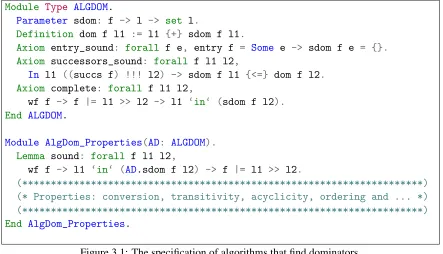
Figure 3.1 gives an abstract specification of algorithms that compute dominators using a Coq
module interfaceALGDOM. First of all,sdomdefines the signature of a dominance analysis algorithm:
given a function f and a labell1, (sdom f l1) returns the set of strict dominators ofl1 in f; dom
defines the set of dominators ofl1by addingl1intol1’s strict dominators.
To make the interface simple, ALGDOMrequires only basic properties that ensure thatsdom is
correct: it must be bothsoundandcompletein terms of the declarative definitions (Definition 2).
Efficiency
Lengauer-Tarjan (LT, in LLVM and GCC) Based on graph theory
O(E x log(N)) Cooper-Harvey-Kennedy (CHK)
Extended from AC
Nearly as fast as LT in common cases
Verifiability
Allen-Cocke (AC)Based on Kildall’s algorithm A large asymptotic complexity
Figure 3.2: Algorithms of computing dominators
transitivity, acyclicity, ordering, etc.) from the declarative definitions to the implementations of
sdomanddom. Section 3.4, Section 3.5, Section 4.3 and Chapter 8 show how clients ofALGDOMuse
the properties proven inAlgDom_Propertiesby examples.
ALGDOM requires completeness of the algorithm directly. Soundness of the algorithm can be
proven by two more basic properties:entry_soundrequires that the entry has no strict dominators;
successors_soundrequires that ifl1 is a successor ofl2, then l2’s dominators must includel1’s
strict dominators. Given an algorithm that establishes the two properties, AlgDom_Properties
proves that the algorithm is sound by induction over any path from the entry tol2.
3.1.3 Instantiations
In the literature, there is a long history of algorithms that find dominators (See Figure 3.2), each
making different trade-offs between efficiency and simplicity. Most of the industrial compilers,
such as LLVM and GCC, use the classic Lengauer-Tarjan algorithm [40] (LT) that has a complexity
ofO(E∗log(N))whereNandEare the number of nodes and edges respectively, but is complicated
to implement and reason about because it is base on complicated graph theory. The Allen-Cocke
algorithm [7] (AC) based on iteration is easier to design, but suffers from a large asymptotic
com-plexity of O(N3). Moreover, LT explictly creates dominator trees that provide convenient data
structures for compilers whereas AC needs an additional tree construction algorithm with more
en-entry {e,5}
{a,4}
{d,2} {b,3}
{c,1}
{z,_}
{y,_}
stk visited PO_l2p po
e[a d] e
e[d]; a[b] e a e[d]; a[]; b[c d] e a b
e[d]; a[]; b[d]; c[] e a b c (c,1) e[d]; a[]; b[]; d[b] e a b c d (c,1) e[d]; a[]; b[]; d[] e a b c d (c,1); (d,2) e[d]; a[]; b[]; e a b c d (c,1); (d,2); (b,3) e[d]; a[]; e a b c d (c,1); (d,2); (b,3); (a,4) e[] e a b c d (c,1); (d,2); (b,3); (a,4); (e,5)
Figure 3.3: The postorder (left) and the DFS execution sequence (right).
gineering and runs nearly as fast as LT in common cases [24, 31], but is still simple to implement
and reason about. Moreover, CHK generates dominator trees implicitly, and provides a faster tree
construction algorithm.
Because CHK gives a relatively good trade-off between verifiability and efficency, we present
CHK as an instance ofALGDOM. In the following sections, we first review the AC algorithm, and
then study its extension CHK.
3.2
The Allen-Cocke Algorithm
The Allen-Cocke algorithm (AC) is an instance of the forward worklist-based Kildall’s
al-gorithm [35] that computes program fixpoints by iteration. The number of iterations that a
worklist-based algorithm takes to meet a fixpoint depends on the order in which nodes are
processed: in particular, forward algorithms can converge relatively faster when visiting nodes in
reverse postorder (PO) [33].
At the high-level, our Coq implementation of AC works in three steps: 1) calculate the PO of a
CFG by depth-first-search (DFS); 2) compute strict dominators for PO-numbered nodes in Kildall;
3) finally relate the analysis results to the original nodes. We omit the 3rd step’s proofs here.
This section first presents a verified DFS algorithm that computes PO, then reviews Kildall’s
algorithm as implemented in the CompCert project [42], and finally it studies the implementation
Record PostOrder := mkPO { PO_cnt: positive; PO_l2p: LTree.t positive }.
Record Frame := mkFr { Fr_name: l; Fr_scs: list l }.
Definition dfs_F_type : Type := forall (succs: LTree.t (list l))
(visited: LTree.t unit) (po:PostOrder) (stk: list Frame), PostOrder.
Definition dfs_F (f: dfs_F_type) (succs: LTree.t (list l))
(visited: LTree.t unit) (po:PostOrder) (stk: list Frame): PostOrder := match find_next succs visited po stk with
| inr po’ => po’
| inl (next, visited’, po’, stk’) => f succs visited’ po’ stk’
end.
Figure 3.4: The DFS algorithm.
3.2.1 DFS: PO-numbering
DFS starts at the entry, visits nodes as deep as possible along each path, and backtracks when all
deep nodes are visited. DFS generates PO by numbering a node after all its children are numbered.
Figure 3.3 gives a PO-numbered CFG. In the CFG, we represent the depth-first-search (DFS) tree
edges by solid arrows, and non-tree edges by dotted arrows. We draw the entry node in a box, and
other nodes in circles. Each node is labeled by a pair with its original label name on the left, and its
PO number on the right. Because DFS only visits reachable nodes, the PO numbers of unreachable
nodes are represented by ‘ ’.
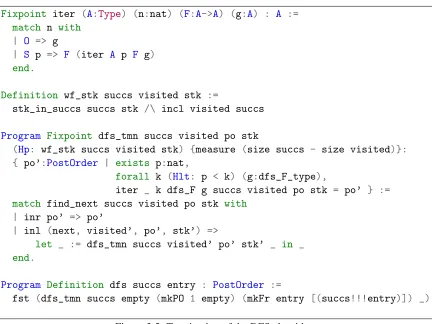
Figure 3.4 shows the data structures and auxiliary functions used by a typical DFS algorithm
that maintains four components to compute PO.PostOrdertakes the next available PO number and
a map from nodes to their PO numbers with typepositive. The map from a node to its successors
is represented bysuccs. To facilitate reasoning about DFS, we represent the recursive information
of DFS explicitly by a list ofFramerecords that each contains a nodeFr_nameand its unprocessed
successorsFr_scs. To prevent the search from revisiting nodes, the DFS algorithm usesvisited
to record visited nodes.dfs_Fdefines one recursive step of DFS.
Figure 3.3 (on the right) gives a DFS execution sequence (by runningdfs_Funtil all nodes are
visited) of the CFG in Figure 3.3 (on the left) . We usel[l1· · ·ln]to denote a frame with the nodel
and its unprocessed successorsl1toln;(l,p)to denote a nodeland its POp. Initially the DFS adds
Fixpoint iter (A:Type) (n:nat) (F:A->A) (g:A) : A := match n with
| O => g
| S p => F (iter A p F g) end.
Definition wf_stk succs visited stk :=
stk_in_succs succs stk /\ incl visited succs
Program Fixpoint dfs_tmn succs visited po stk
(Hp: wf_stk succs visited stk) {measure (size succs - size visited)}: { po’:PostOrder | exists p:nat,
forall k (Hlt: p < k) (g:dfs_F_type),
iter _ k dfs_F g succs visited po stk = po’ } := match find_next succs visited po stk with
| inr po’ => po’
| inl (next, visited’, po’, stk’) =>
let _ := dfs_tmn succs visited’ po’ stk’ _ in _ end.
Program Definition dfs succs entry : PostOrder :=
fst (dfs_tmn succs empty (mkPO 1 empty) (mkFr entry [(succs!!!entry)]) _).
Figure 3.5: Termination of the DFS algorithm.
node that is the unvisited node in theFr_scsof the latest nodel0of the stack. If the next available node exists, the DFS pushes the node with its successors to the stack, and makes the node to be
visited. find_nextpops all nodes in front ofl0, and gives them PO numbers. Iffind_nextfails to find available nodes, the DFS stops.
We can see that the straightforward algorithm is not a structural recursion. To implement
the algorithm in Coq, we must show that it terminates. Although in Coq we can implement the
algorithm by well-founded recursion, such designs are hard to reason about [17]. One of possible
alternatives is implementing DFS with a ‘strong’ dependent type to specify the properties that we
need to reason about DFS. However, this design is not modular because when the type of DFS
is not strong enough—for example, if we need a new lemma about DFS—we must extend or
redesign its implementation by adding new invariants. Instead, following the ideas in Coq’Art [17],
we implement DFS by iteration and prove its termination and inductive principle separately. By
Figure 3.5 presents our design. Similar to bounded iteration, the top-level entry isiter, which
needs a bounded stepn, a fixpointFand a default valueg. iteronly callsgwhennreaches zero,
and otherwise recursively calls one more iteration ofF. IfFis terminating, we can prove that there
must exist a final value and a boundn, such that for any boundkthat is greater than or equal ton,
iteralways stops and generates the same final value. In other words,Fmust reach a fixpoint with
less thannsteps. In fact, the proof of the existence of nis erasable; the computation part of the
proof provides a terminating algorithm for free, not requiring the bound step at runtime.
Figure 3.5 proves that the DFS must terminate, as shown bydfs_tmn, which is implemented
by well-founded recursion over the number of unvisited nodes. Intuitively, this follows because
after each iteration, the DFS visits more nodes. The invariant that the number of unvisited nodes
decreases holds only for well-formed recursion states (wf_stk), which requires that all visited nodes
and unprocessed nodes in frames must be in the CFG. We implementeddfs_tmnby Coq’sProgram
Fixpoint, which allows programmers to leaveholesfor whichProgram Fixpointautomatically
generates obligations to solve. Usingdfs_tmn,dfsdefines the final definition of DFS.
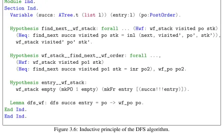
To reason aboutdfs, Figure 3.6 shows a well-founded inductive principle fordfs. InModule
Ind, to prove that the final result has the propertywf_poand the propertywf_stackholds for all its
intermediate states, we need to show that the initial state satisfieswf_stack, and thatfind_next
preserveswf_stackwhen it can find a new available node, and produces a well-formed final result
when no available nodes exist. With the inductive principle, we proved the following properties of
DFS that are useful to establish the correctness of AC and CHK.
Variable (succs: ATree.t (list l)) (entry:l) (po:PostOrder).
Hypothesis Hdfs: dfs succs entry = po.
First of all, a non-entry node must have at least one predecessor that has a greater PO number than
the node’s. This is because 1) DFS must visit at least one predecessor of a node before visiting the
node; 2) PO gives greater numbers to the nodes visited earlier:
Lemma dfs_order: forall l1 p1, l1 <> entry -> (PO_l2p po)!l1 = Some p1,
exists l2, exists p2,
In l2 ((make_preds succs)!!!l1) /\ (PO_l2p po)!l2 = Some p2 /\ p2 > p1. (* Given succs, (make_preds succs) computes predecessors of each node. *)
Second, a node is PO-numbered iff the node is reachable:
Module Ind. Section Ind.
Variable (succs: ATree.t (list l)) (entry:l) (po:PostOrder).
Hypothesis find_next__wf_stack: forall ... (Hwf: wf_stack visited po stk) (Heq: find_next succs visited po stk = inl (next, visited’, po’, stk’)),
wf_stack visited’ po’ stk’.
Hypothesis wf_stack__find_next__wf_order: forall ..., (Hwf: wf_stack visited po1 stk)
(Heq: find_next succs visited po1 stk = inr po2), wf_po po2.
Hypothesis entry__wf_stack:
wf_stack empty (mkPO 1 empty) (mkFr entry [(succs!!!entry)]).
Lemma dfs_wf: dfs succs entry = po -> wf_po po. End Ind.
End Ind.
Figure 3.6: Inductive principle of the DFS algorithm.
Moreover, different nodes do not have the same PO number.
Lemma dfs_inj: forall l1 l2 p,
(PO_l2p po)!l2 = Some p -> (PO_l2p po)!l1 = Some p -> l1 = l2.
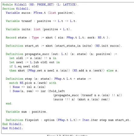
3.2.2 Kildall’s algorithm
Figure 3.7 summarizes the Kildall module used in the CompCert project. The module is
param-eterized by the following components: NSthat provides the order to process nodes, and a latticeL
that definestop,bot, equality (eq), least upper bound (lub) and order (ge) of the abstract domain
of an analysis;succsthat is a tree that maps a node to their successors;transfthat is the transfer
function of Kildall analysis;initsthat initializes the analysis. Given the inputs,staterecords the
iteration states that includesinthat records analysis states of each node, and a work listswrkhat
contains nodes to process.
fixpointimplements iterations byIter.iter—bounded recursion with a maximal step
num-ber (num) [17].Iter.iteris partial if an analysis does not stop after the maximal number of steps.
A monotone analysis must reach its fixpoint after a fixed number of steps. Therefore, we can alway
Module Kildall (NS: PNODE_SET) (L: LATTICE). Section Kildall.
Variable succs: PTree.t (list positive).
Variable transf : positive -> L.t -> L.t.
Variable inits: list (positive * L.t).
Record state : Type := mkst { sin: PMap.t L.t; swrk: NS.t }.
Definition start_st := mkst (start_state_in inits) (NS.init succs).
Definition propagate_succ (out: L.t) (s: state) (n: positive) := let oldl := s.(sin) !! n in
let newl := L.lub oldl out in if L.eq newl oldl
then mkst (PMap.set n newl s.(sin)) (NS.add n s.(swrk)) else s.
Definition step (s: state): PMap.t L.t + state := match NS.pick s.(swrk) with
| None => inl s.(sin)
| Some(n, rem) => inr (fold_left
(propagate_succ (transf n s.(sin) !! n)) (succs !!! n) (mkst s.(sin) rem))
end.
Variable num : positive.
Definition fixpoint : option (PMap.t L.t):= Iter.iter step num start_st. End Kildall.
End Kildall.
Figure 3.7: Kildall’s algorithm.
Initially Kildall’s algorithm callsstart_stto initialize iteration states. Nodes not ininitsare
initialized to be the bottom ofL. Thenstart_stadds all nodes into the worklist and starts the loop.
stepdefines the loop body. Atstep, Kildall’s algorithm checks if there are still unprocessed nodes
in the worklist. If the worklist is empty, the algorithm stops. Otherwise,step picks a node from
the worklist in term of the order provided byNS, and then propagates its information (computed by
a successor isL.lubof its old value and the propagated value from its predecessor. The algorithm
only adds a successor into the worklist when its value is changed.
Kildall’s algorithm satisfies the following properties:
Variable res: PMap.t L.t.
Hypothesis Hfix: fixpoint = Some res.
First of all, the worklist contains nodes that have unstable successors in the current state. Formally,
each statestpreserves the following invariant:
forall n, NS.In n st.(swrk) \/
(forall s, In s (succs!!!n) -> L.ge st.(sin)!!s (transf n st.(sin)!!n)).
Each iteration may only remove the picked node nfrom the worklist. If none ofn’s successors’
values are changed, no matter whethernbelongs to its successors, nwon’t be added back to the
worklist. Therefore, the above invariant holds. This invariant implies that when the analysis stops,
all nodes hold the in-equations:
Lemma fixpoint_solution: forall s,
In s (succs!!!n) -> L.ge res!!s (transf n res!!n).
The second property of Kildall’s algorithm ismonotonicity. At each iteration, the value of a
suc-cessor of the picked node can only be updated fromoldltonewl. Becausenewlis the least upper
bound ofoldlandout,newlis greater than or equal tooldl. Therefore, iteration states are always
monotonic:
Lemma fixpoint_mono: incr (start_state_in inits) res.
whereincris a pointwise lift ofL.gefor corresponding nodes. In particular, the final states must
be greater than or equal to the initial states. When an iteration does not change states, no nodes
will be added back to the worklist, but the size of worklist must decrease. Therefore, a monotonic
analysis must reach its fixpoint with less thanN2∗H steps whereN is the number of nodes;H is
the height of the lattice of the analysis [33].
3.2.3 The AC algorithm
AC instantiatesKildall withPN that picks nodes in reverse PO (by picking the maximal nodes
from the worklist), andLDoms that defines the lattice of AC. Dominance analysis computes a set
topand botof LDomsare Some nil andNone respectively. The least upper bound, order and
equality ofLDomsare lifted from set intersection, set inclusion, and set equality tooption:Noneis
smaller thanSome xfor anyx. This design leads to better performance by providing shortcuts for
operations onNone. Note that usingNoneasbotdoes not make the height ofLDomsto be infinite,
because any non-botelement can only contain nodes in the CFG, and the height ofLDomsisN.
AC uses the following transfer function and initialization:
Definition transf l1 input := l1 {+} input.
Definition inits := [(e, LDoms.top)].
Initially AC sets the strict dominators of the entry to be empty, and other nodes’ strict dominators
to be all labels in the function. The algorithm will iteratively remove non-strict-dominators
from the sets until the conditions below hold (by Lemma fixpoint_mono and Lemma
fixpoint_solution):
(forall s, In s (succs!!!n) ->
L.ge (st.(sin))!!s (n{+}(st.(sin))!!n)) /\ (st.(sin))!!e = {}.
which proves that AC satisfiesentry_soundandsuccessors_sound.
To show that the algorithm is complete, it is sufficient to show that each iteration state st
preserves the following invariant:
forall n1 n2, ~ n1 ‘in‘ st.(sin)!!n2 -> ~ (e, succs) |= n1 >> n2.
In other words, AC only removes non-strict dominators. Initially, AC sets the entry’s strict
dom-inators to be empty. Because in a well-formed CFG, the entry has no predecessors, the invariant
holds at the very beginning. At each iteration, suppose that we pick a nodenand update one of its
successorss. Consider a node n’not inLDoms.lub st.(sin)!!s (n {+} st.(sin)!!n). If
n’is not inLDoms.lub st.(sin)!!s, thenn’does not strictly dominatesbecausestholds the
invariant. Ifn’is not in(n {+} st.(sin)!!n), thenn’does not strictly dominatenbecausest
holds the invariant. Appending the path from the entry tonthat bypassesn’with the edge fromn
tosleads to a path from the entry tosthat bypassesn’. Therefore,n’does not strictly dominate
3.3
Extension: the Cooper-Harvey-Kennedy Algorithm
The CHK algorithm is based on the following observation: when AC processes nodes in a reversed
post-order (PO), if we represent the set of strict dominators in a list, and always add a newly
discovered strict dominator at the head of the list (on the left in Figure 3.8), the list must be sorted
by PO. Figure 3.8 (on the right) shows the execution of the algorithm for the CFG in Figure 3.3.
Because lists of strict dominators are always sorted, we can implement the set intersection (lub)
and the set comparison (eq) of two sorted lists by traversing the two lists only once. Moreover, the
algorithm only callseqafterlub. Therefore, we can grouplubandeqintoLDoms.lubtogether.
The following defines a merge function used byLDoms.lub that intersects two sorted lists and
returns whether the final result equals to the left one:
Program Fixpoint merge (l1 l2: list positive) (acc:list positive * bool) {measure (length l1 + length l2)}: (list positive * bool) :=
let ’(rl, changed) := acc in match l1, l2 with
| p1::l1’, p2::l2’ =>
match (Pcompare p1 p2 Eq) with
| Eq => merge l1’ l2’ (p1::rl, changed)
| Lt => merge l1’ l2 (rl, true)
| Gt => merge l1 l2’ (rl, changed)
end
| nil, _ => acc
| _::_, nil => (rl, true)
end.
(* (Pcompare p1 p2 Eq) returns whether p1 = p2, p1 < p2 or p1 > p2. *)
3.3.1 Correctness
To show that CHK is still correct, it is sufficient to show that all lists are well-sorted at each iteration,
which ensures that the abovemergecorrectly implements intersection and comparison. First, if a
node with numbernstill maps tobot, the worklist must contain one of its predecessors that has a
entry {e,5}
{a,4}
{b,3}
{d,2} {c,1}
Nodes sin
5 [] [] [] [] [] [] [] [] []
4 · [5] [5] [5] [5] [5] [5] [5] [5]
3 · · [45] [45] [45] [5] [5] [5] [5]
2 · · · [345] [345] [345] [35] [35] [35]
1 · [5] [5] [5] [5] [5] [5] [5] [5]
swrk [54321] [4321] [321] [21] [1] [3] [21] [1] []
Figure 3.8: The dominator trees (left) and the execution of CHK (right).
forall n, in_cfg n succs -> (st.(sin))!!n = None ->
exists p, In p ((make_preds succs)!!!n) /\ p > n /\ PN.In p st.(st_wrk). (* in_cfg checks if a node is in CFG. *)
This invariant holds in the beginning because all nodes are in the worklist. At each iteration, the
invariant implies that the picked node n with the maximal number inst.(st_wrk)is not bot.
Suppose it isbot, there cannot be any node with greater number in the worklist. This property
ensures that after each iteration, the successors ofncannot bebot, and that the new nodes added
into the worklist cannot bebot, because they must be those successors. Therefore, the predecessors
of the remainingbotnodes still in the worklist cannot ben. Since onlynis removed, the rest of the
botnodes still hold the above invariant.
In the algorithm, a node’s value is changed from bot to non-bot when one of its non-bot
predecessors is processed. With the above invariant, we know that the predecessor must be of larger
number. Once a node turns to be non-bot, no new elements will be added in its set. Therefore,
this implies that, at each iteration, if the value of a node is notbot, then all its candidate strict
dominators must be larger than the node:
forall n sdms, (st.(sin))!!n = Some sdms -> Forall (Plt n) sdms. (* Plt is the less-than of positive. *)
Moreover, a nodenis considered as a candidate of strict dominators originally bytranfthat
always consnat the head of (st.(sin))!!n. Therefore, we proved that the non-botvalue of a
node is always sorted:
Inductive DTree : Set :=
| DT_node : l -> DTrees -> DTree
with DTrees : Set :=
| DT_nil : DTrees
| DT_cons : l -> DTrees -> DTrees. Variable (f: function) (entry:l).
Inductive wf_dtree : DTree -> Prop :=
| Wf_DT_node : forall l0 dts (Hrd: f |= entry ->* l0)
(Hnotin: ~ l0 ‘in‘ (dtrees_dom dts)) (Hdisj: disjoint_dtrees dts) (Hidom: forall_children idom l0 dts) (Hwfdts: wf_dtrees dts),
wf_dtree (DT_node l0 dts)
(* (dtrees_dom dts) returns all labels in dts. *) (* (disjoint_dtrees dts) ensures that labels of dts are disjointed. *) (* (forall_children idom l0 dts)) checks that l0 immediate-dominates all *)
(* roots of dts. *)
with wf_dtrees : DTrees -> Prop :=
| Wf_DT_nil : wf_dtrees DT_nil
| Wf_DT_cons : forall dt dts (Hwfdt: wf_dtree dt) (Hwfdts: wf_dtrees dts),
wf_dtrees (DT_cons dt dts).
Figure 3.9: The definition and well-formedness of dominator trees.
3.4
Constructing Dominator Trees
In practice, compilers construct dominator trees from dominators, and analyze or optimize
programs by recursion on dominator trees.
Definition 3.
• A block l1is animmediate dominatorof a block l2, written G|=l1≫l2, if G|=l1l2and
(∀G|=l3l2,G|=l3=l1).
• A tree is called adominator treeof G if the tree has an edge from l to l0iff G|=l≫l0.
Figure 3.8 shows the dominator tree of the CFG in Figure 3.3. In Figure 3.8, solid edges
represent tree edges, and dotted edges represent non-tree but CFG edges.
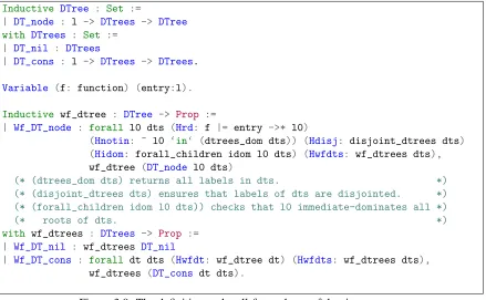
Formally, we define dominator trees in Figure 3.9 that has the inductive well-formed
(wf_dtree) property with which we can reason about recursion on dominator trees: given a tree
nodel, 1)lis reachable; 2)lis different from all labels inl’s descendants; 3) labels ofl’s subtrees
Consider the final analysis results of CHK in Figure 3.8, we can see that for each node, its list
of strict dominators exactly presents a path from root to the node on the dominator tree. Therefore,
we can construct a dominator tree by merging the paths. We proved that the algorithm correctly
constructs a well-formed dominator tree (See our code). For the sake of space, we only present
that each tree edge represents≫ by showing that for any nodelin the final state, the list ofl’s
dominators must be sorted by≫.
We first show that the list is sorted by . Consider two adjacent nodes in the list, l1 and
l2, such that l1 <l2. Because of soundness, G|=l1 =l and G|=l2 =l. By Lemma 5,
G|=l2 l1∨G|=l1 l2. Suppose G|=l1 l2, by completeness, l1 must be in the strict
dominators computed forl2, and therefore, be greater than l2. This is a contradiction. Then, we
prove that the list is sorted by≫. SupposeG|=l3l1. By Lemma 1 and Lemma 2,G|=l3l.
By completeness,l3must be in the list. We have two cases:
1. l3≥l2: Because the list is sorted by,G|=l3=l2.
2. l3≤l1: Similarly,G|=l1=l3. This is a contradiction by Lemma 4.
3.5
Dominance Frontier
Another application of computing dominators is the calculation of dominance frontiers that has
applications to SSA construction algorithms, computing control dependence, andetc.
Cytronet al.define the dominance frontier of a node,b, as:
... the set of all CFG nodes,y, such thatbdominates a predecessor ofybut does not strictly dominatey[28].
They propose finding the dominance frontier set for each node in a two step manner. They begin
by walking over the dominator tree in a bottom-up traversal. At each node, b, they add to b’s
dominance-frontier set any CFG successors not dominated byb. They then traverse the
dominance-frontier sets ofb’s dominator-tree children each member of these frontiers that is not dominated by
bis copied intob’s dominance frontier.
We follow an algorithm designed by Cooper, Harvey and Kennedy [24] that approaches the
problem from the opposite direction, and tends to run faster than Cytronet al.’s algorithm in
0% 50% 100% 150% 200% 250%
Overhead over LLVM
CHK-tree CHK AC-tree AC
go
compress ijpeg gzip vpr mesa artammpequake256.bzip2parser twolf401.bzip2 gcc mcfhmmerlibquantum lbm milc sjengh264refGeo. mean
Figure 3.10: Analysis overhead over LLVM’s dominance analysis for our extracted analysis.
join points in the graph, nodes into which control flows from multiple predecessors. Second, the
predecessors of any join point, j, must have j in their respective dominance-frontier sets, unless
the predecessor dominates j. This is a direct result of the definition of dominance frontiers, above.
Finally, the dominators of j’s predecessors must themselves have jin their dominance-frontier sets
unless they also dominate j.
These observations lead to a simple algorithm. First, we identify each join point, j—any node
with more than one incoming edge is a join point. We then examine each predecessor, p, of j
and walk up the dominator tree starting at p. We stop the walk when we reach j’s immediate
dominator—jis in the dominance frontier of each of the nodes in the walk, except forj’s immediate
dominator. Intuitively, all of the rest of j’s dominators are shared by j’s predecessors as well. Since
they dominate j, they will not have jin their dominance frontiers.
As shown previously [24], this approach tends to run faster than Cytronet al..’s algorithm in
practice, almost certainly for two reasons. First, the iterative algorithm has already built the
domina-tor tree. Second, the algorithm uses no more comparisons than are strictly necessary. Section 8.5.3
will revisit the implementation of the algorithm.
3.6
Performance Evaluation
As we discussed, computing dominators is crucial in SSA-based compilers. Therefore, we use the
Instance Analysis Times (s)
Name Vertices Edges LT CHK CHK-tree AC AC-tree idfsquad 6002 10000 0.08 10.54 24.87
ibfsquad 4001 6001 0.14 11.38 13.16 12.43 30.00 itworst 2553 5095 0.14 8.47 11.22 19.16 69.72 sncaworst 3998 3096 0.19 17.03 32.08 205.07 740.53
Table 3.1: Worst-case behavior.
of the resultant code on a 1.73 GHz Intel Core i7 processor with 8 GB memory running benchmarks
selected from the SPEC CPU benchmark suite that consist of over 873k lines of C source code.
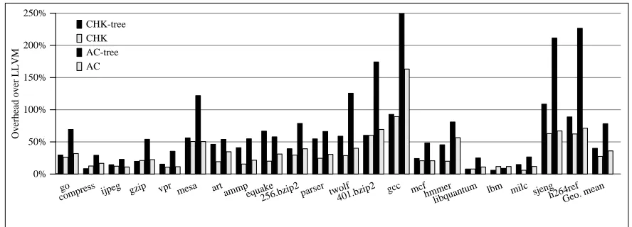
Figure 3.10 reports the analysis time overhead (smaller is better) over the C++ version of LLVM
dominance analysis (which uses LT) baseline. LT only generates dominator trees. Given a
domina-tor tree, the strict dominadomina-tors of a tree node are all the node’s ancesdomina-tors. The second left bar of each
group shows the overhead of CHK, which provides an average overhead of 27%. The right-most
bar of each group is the overhead of AC, which provides 36% on average.
To study the asymptotic complexity, Table 3.1 shows the result of graphs that elicit the
worst-case behavior used previously [31]. On average, CHK is 86 times slower than LT. The ‘ ’ indicates
that the running time is too long to collect. For the testcases on which AC stops, AC is 226 times
slower than LT.
The results of CHK match earlier experiments [24, 31]: in common cases, CHK runs nearly
as fast as LT. For programs with reducible CFGs, a forward iteration analysis in reverse PO will
halt in no more than size passes [33], and most CFGs of the common benchmarks are reducible.
The worst-case tests contain huge irreducible CFGs. Different from these experiments, AC does
not provide large overhead, because we useNoneto representbot, which provides shortcuts for set
operations.
As shown in Section 3.4, CHK computes dominator trees implicitly, while AC needs additional
costs to create dominator trees. Figure 3.10 and Table 3.1 also report the performance of the
dominator tree construction. CHK-tree stands for the algorithm that first computes dominators
by CHK and then runs the tree construction defined in Section 3.4. AC-tree stands for the algorithm
that first computes dominators by AC, sorts strict dominators for each node, and then runs the same
tree construction. For common programs, on average, CHK-tree provides an overhead 40% over