OPTIMAL NODE PLACEMENT IN
WIRELESS SENSOR NETWORKS
G.Pradeep Reddy1
Asst. Professor, Lovely Honours School of Technology (ECE) Lovely Professional University, Jalandhar, Punjab, Pin: 144402, India.
Gerardine Immaculate Mary2
Asst. Prof. (Sr.), School of E lectronic s Engine eri ng VIT Uni versit y, Vellore, Pi n: 632014, India.
Abstract:
Judicious deployment of fixed anchors (node with known positions) is to be considered in sensor networks which are used for monitoring and detecting a possible hazardous event in underground mines (such as fire, flammable, explosive, toxic gas); UWB is selected owing to its asset in ranging accuracy, pre-eminently in cluttered environments compared to other technology, and their ability to penetrate obstacles. It is therefore the signal of choice for many indoor ranging. This paper proposes a low complexity parameter to determine the optimal placement of sensor nodes, measurement results using ZigBeeTM specification are shown as proof of concept that precise channel profiles between different LOS and NLOS conditions can be identified with this combined strategy.
Keywords: UWB channel profile identification; optimal sensor node placemen; IEEE 802.15.4a Channel Model.
I. Introduction
Sensor networks have been proposed for various applications due its ability for monitoring and detecting a possible hazardous event in underground mines such as fire, flammable, explosive, toxic gas; where judicious deployment of fixed anchors (node with known positions) is to be considered. In emergencies wireless communication may become vital for survival, for example, during a disaster such as a fire, rock falls, the conventional wired communication system may become unreliable, necessitating a wireless radio system. A wireless sensor network is composed of sensors which are deployed across a geographical area. Each sensor can be thought of as having two important modules. The first is the sensing module depending on the mission at hand (i.e., seismic, chemical, temperature, etc.). The second is the wireless communication module, which is used to communicate with the other sensors in ad-hoc fashion.
One of the most promising applications for UWB is sensor networks, where a large number of sensor nodes communicate among each other, and with central nodes, with high reliability. The data rates for those applications are typically low (1Mbit/s), and the good ranging and geolocation capabilities of UWB are particularly useful. Recognizing these developments, the IEEE has established the standardization group 802.15.4a, which is currently in the process of developing a standard for these applications.
Intuitively, to find the best receiver position in indoor environments where the sensors get the optimum signal to be detected, the following may be considered, either the position where best signal is received or average of all multipath signals received at a point or alternatively SNR may be used.
Table1: Optimum receiver position using other measures like best signal strength and average value.
Position 1 Position 2
50 50
25 40
35 40
30 10
10 10
Average = 50 Average =50
If the best signal received is considered, best signals may be got at different positions of the receiver, and the better of the two cannot be identified.
If average value of received signals is considered to find the best receiver position, the predicament is same, as shown in the table, where the average values of received signals at two receiver positions 1 and 2 are equal.
If the SNR is considered to find the best receiver positions, the following are the limitations, first, it is difficult to estimate the SNR, secondly using only SNR of the received signal doesn’t account for the individual channel realizations.
Thus the above methods will not give the optimised receiver position. The best receiver positions can be determined by using the kurtosis index. The kurtosis index captures both the statistics of individual channel realizations and SNR of the received signal. Thus receiver can be placed where the kurtosis index is maximum. In the above example, the two positions shown have different kurtosis indices, at position 1, κ =2.22 and at position 2, κ =1.27, so position 1 can besuggested as the best receiver position. The example can be extended to many such receiver positions and can be noted that in the case of considering only best signal strength or only best SNR measures, we may get many similar values to decide from, whereas using kurtosis index as the parameter, less number of similar values occur, making the decision of optimum receiver position easier.
II. Related Work
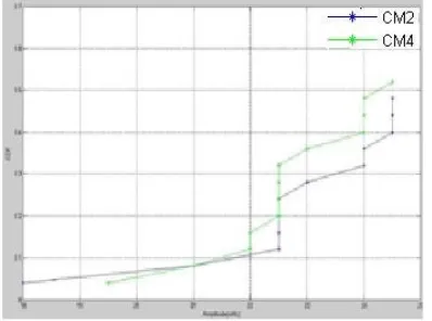
Earlier, CDF (cumulative distribution function) was used to identify the indoor channels profiles, between LOS and NLOS. The CDF of the variable X is defined as the probability that X assumes any value smaller then x, i.e. P(X<x) = F(x). But the CDF can differentiate only LOS and NLOS paths and not between different LOS and NLOS paths, more over it needs estimation algorithm to estimate the channels and the CDF of the rooms looks closer, where we can’t differentiate the channels precisely as shown in results(Fig.3).
Kurtosis index is proposed as the appropriate parameter to differentiate the indoor channels effectively and thereby identify the best receiver position in indoor environments.
III. Kurtosis Index
Kurtosis Index κ is a low complexity parameter [6] able to precisely discriminate channels. More over the parameter κdoes not need any application of estimation algorithms on the received signal because it is calculated directly by the received signal sample.
It is defined as “A statistical parameter that indicates the fourth order moment of the received signal amplitude”
κ (x)=
∑ ̅
(1)
where is received signal N is number of samples
is variance and = ∑ ̅ ̅ is the mean
As the variance parameter is in denominator of the kurtosis index, it is possible to differentiate the channels precisely, for the low variance values also.
IV. Standard UWB Indoor Channel Models
communications are best suited for short-range communications: sensor networks and personal area networks (PANs).
The multipath model of the standard is based on the large number of the measurement campaigns. This UWB channel model is calculated based on the modified Saleh-Valenzuela model [4]. The standard recommends using a log normal distribution rather than Rayleigh distribution. The discrete time –impulse response can be written as
ℎ= ∑ ∑ ,δ(t−− , ) (2)
Where
• , is the multipath gain coefficients of the !"path, within the #!"cluster in the $!"realization.
• , is the delay of the #!"cluster in the $!"realization.
• , is the delay of the !"multipath component relative to the #!"cluster arrival time . • Represents the log-normal shadowing, and i refer to the i threalization.
The following environments have a high importance for sensor network applications and are those ones for which the model is parameterized
1) Indoor residential: These environments are critical for “home networking,” linking different appliances, as
well as safety (fire, smoke) sensors over a relatively small area. The building structures of residential environments are characterized by small units, with indoor walls of reasonable thickness.
2) Indoor office: Some of the rooms are comparable in size to residential, but other rooms (especially cubicle areas, laboratories, etc.) are considerably larger. Areas with many small offices are typically linked by long corridors. Each of the offices typically contains furniture, bookshelves on the walls, etc., which adds to the attenuation given by the (often thin) office partitioning.
3) Outdoor: While a large number of different outdoor scenarios exist, the current model covers only a suburban-like microcell scenario, with a rather small range.
4) Industrial environments: Characterized by larger enclosures (factory halls), filled with a large number of metallic reflectors. This is anticipated to lead to severe multipath.
5) Agricultural areas/farms:For those areas, few propagation obstacles (silos, animal pens), with large distances in between, are present. The delay spread can thus be anticipated to be smaller than in other environments.
V. UWB Signal Modelling
The most common pulse shapes for Impulse-UWB work are the Gaussian pulse and its derivatives, since they are easy to describe and work with. The Gaussian pulse is described by
% =√Π' )
*+,-.
(3)
Where is the variance parameter. The pulse width is given by the expression, /=2Πσ.
Another pulse model is the first derivative of the Gaussian pulse. This is used as a model since a UWB antenna may have the effect on the signal to be equivalent to differentiating the pulse with respect to the time variable. Letting the mean value be zero, the first derivative is given by,
%(t)= − 0√Π'! 12)* +,
-. (4)
The third model is based on the second derivative of the Gaussian pulse and given by,
%(t)= A0 !
√Π3−√Π 12)
*+,-.
(5)
VI. Simulation
VII. Experimental Setup
ZigBeeTM transmitting module is in a fixed position throughout the experiment and the receiving module is positioned in four different rooms as per the channel model-specific distance criteria [4]. The received signal strengths are measured, from which kurtosis indices are obtained. In each room 25 grid locations are used for different receiver positions, within one square meter area and the distance between each grid is 25cm. The results are shown in Fig.2.
VIII. Simulation Results
The UWB signal is modelled as Gaussian and simulated as shown in Fig.1.
Fig.1 UWB signal at the channel input
IX. Experimental Results
Fig.2 Kurtosis indices and their mean values calculated over 25 grid locations by real measurements.
These results using kurtosis index as the parameter proved better channel profile identification when compared to the results obtained using CDF (Fig.3) for the same purpose. By using CDF as the parameter to identify two NLOS channel models (CM2 and CM4), it found that the two channel models are not easily distinguishable.
Fig. 3 Cumulative Distribution functions of best paths for CM2 and CM4 by real measurements.
X. Conclusions
In this paper a low complexity parameter, kurtosis index is proposed to identify the best node placement in wireless sensor network environments. The Indoor channel models (CM1, CM2, CM3, and CM4) are effectively identified between different LOS and NLOS conditions.
XI. Acknowledgments
We are thankful to the Mr. Gaurav Sethi, COD, LSHT-ECE, Lovely Professional University for the support during this work.
XII. References
[1] C. Falsi, D. Dardari, L. Mucchi, M. Z. Win, “Time of arrival estimation for UWB localizers in realistic environments," EURASIP J. Applied Signal Processing, Special Issue on Wireless Location Technologies Applications, vol. 2006 , article ID 32082,
[2] D. Cassioli, M. Z. Win, and A. F. Molisch, “The ultra-wide bandwidth Indoor channel: from statistical model to simulations," IEEE J. Select Areas Commun., vol. 20, no. 6, pp. 1247-1257, Aug. 2002.
[4] A. F. Molisch et al., “A comprehensive standardized model for ultrawideband propagation channels," IEEE Trans. Antennas Propag., vol. 54, no. 11, part 1, pp. 3151-3166, Nov. 2006.
[5] Sami Vahamaa, “Skewness and Kurtosis Adjusted Black-Scholes Model: Hedging Performance”, University of Vaasa, Finland. [6] Lorenzo Mucchi and Patrizio Marcocci,“A New Parameter for UWB Indoor Channel Profile Identification”, IEEE Transactions on
Wireless Communications, Vol. 8, no. 4, April 2009.
Biography of Authors:
G.Pradeep Reddy received his M.Tech degree with specialization in Communication Engineering in Vellore Institute of Technology (VIT), Vellore. He is currently working as Assistant Professor in Lovely Professional University (LPU), Jalandhar, Punjab.