The Scalability Metric based on Cost-Effectiveness in
Distributed Systems
Emmanuel Kwabena
Gyasi
Department of Computer Science
KNUST, Ghana
Dominic Asamoah
Department of Computer Science
KNUST, Ghana
Emmanuel Ofori
Oppong
Department of Computer Science
KNUST, Ghana
Stephen Opoku
Oppong
Faculty of Computing and Information Systems
GTUC, Ghana
ABSTRACT
Today’s computer systems are more complex, more rapidly evolving, and more essential to the conduct of business than those of recent past. The complexity becomes more rigid in the case of distributed systems. As businesses grow, the systems that support their functions also need to grow to support more users, process more data, or both. As they grow, it is important to maintain their performance in terms of responsiveness or throughput. Despite its importance, scalability is poorly understood and few organizations understand how to quantitatively evaluate an application’s scalability. The derived scalability metric of this paper is based on cost effectiveness, in which the effectiveness is a function of the system's throughput and its QoS. It is a strategy based scalability metric that generalizes the well-known metrics for scalability of parallel computations to describe heterogeneous distributed systems. Scalability is measured by the range of scale factors that gives a satisfactory value of the metric, since a good scalability is a joint property of the initial design and the scaling strategy. What makes this derived metric unique is the fact that, it separates the impact of throughput and response time on the metric, formalizing the notation of a scaling strategy, introducing QoS evaluation and more also, introducing formal scalability enablers which are optimized at each scale factor.
Keywords
Distributed Systems, Scalability, Quality of Service, Parallel Computations
1.
INTRODUCTION
Today’s computer systems are more complex, more rapidly evolving, and more essential to the conduct of business than those of even a few years ago. The result is anincreasing need for tools and techniques that assist in understanding the behavior of these systems. Such an understanding is necessary to provide intelligent answers to the questions of cost and performance that arise throughout the life of a system. Right from Scientific institutions, Computer manufacturing industries, businesses of all kinds, educational institutions (Universities), software programmers to individuals, the issue of scalability remains the number one priority in terms of manufacturing and the use of computer systems. This question is of great significance to the organizations involved, because of its potentially serious repercussions from incorrect answers. Unfortunately, this question is also complex as correct answers are not easily obtained.
The world has now become a global village through internet and inter-connectivity. Individuals, organizations, governments, businesses to mention but a few in one way or the other connect or communicate remotely. Businesses have spread up to the extent of defying geographical boundaries whiles individuals and organizations do transact business and at the same time stores their data remotely. Typical example that readily come in mind is cloud computing. These activities are made possible because the system is distributed. A distributed system is a collection of independent computers that appear to its users as a single coherent system. In order words, a distributed system is a collection of independent computers that are used jointly to perform a single task or to provide a single service. Most distributed systems are scalable including present and future applications of which web based distributed systems is no exception. Typical applications, e-commerce, multimedia news services, distance learning, remote medicine, enterprise management, and network management are also some of the examples of distributed services. A distributed system should be deployable in a wide range of scales, in terms of numbers of users and services, quantities of data stored and manipulated, rates of processing, numbers of nodes, geographical coverage, and sizes of networks and storage devices. As businesses grow, the systems that support their functions also need to grow to support more users, process more data, or both. As they grow, it is important to maintain their performance in terms of responsiveness or throughput. Poor performance in these applications often translates into appreciable costs. Customers will oftenshop elsewhere rather than endure long waits. Slow responses in CRM applications mean that more customer-service representatives are needed. And, failure to process financial tradesin a timely fashion can result in statutory penalties as well as lost customers. Despite its importance, scalability is poorly understood and few organizations understand how to quantitatively evaluate an application’s scalability. As a result, they often make assumptions about the scalability of their software. If wrong, these assumptions can be costly.
Many scaled systems suffer from the problem of maintaining productivity and that of delay in transmitting data from one system to another. In the field of telecommunication industry, frequent call drops coupled with high cost of managing distributed networks is a major headache to the managers in telecommunication business as more often than not, scaled networks performance does not commensurate with the cost incurred by scaling the systems, due to unavailable well laid down scalable metrics.
To have metrics that will maintain productivity as the system is scaled so as to enhance call-processing system and make it scalable in order to support large number of callers per hour at an appreciable throughput and at the same time curtail frequent call drops.
To come out with an efficient scalability metrics that ensures cost-effectiveness in distributed systems as the system is been scaled.
To have a detailed welllaid down metric that even an individual can follow in order to scale his/her system.
2.
LITERATURE REVIEW
Different scalability metrics have been developed for massively parallel computation, to evaluate the effectiveness of a given algorithm running on different sized platforms, and to compare the scalability of algorithms. These metrics assume that the program runs by itself, on a set of k
processors with a given architecture, and that the completion time T measures the performance.
2.1
Review of Available Metrics
Performance metrics such as speedup [1], scaled speedup [2], sizeup [3], experimentally determined serial fraction [4], and isoefficiency function [5] have been proposed for quantifying the scalability of parallel systems. While these metrics are extremely useful for tracking performance trends, they do not provide adequate information needed to understand the reason why an algorithm does not scale well on an Architecture. An understanding of the interaction between the algorithmic and architectural characteristics of a parallel system can give us some fair idea. Studies undertaken by Kung [6] and Jamieson [7] help identify some of these characteristics from a theoretical perspective, but that one toodoes not provide any means of quantifying their effects. Severalperformance studies address issues such as latency, contention and synchronization. The limits on interconnection network performance [8], [9] and the scalability of synchronization primitives supported by the hardware [10] , [11] are examples of such studies undertaken over the years. While such issues are extremely important, it is necessary to put the impact of these factors into perspective by considering them in the context of overall application performance. There are studies that use real applications to address specific issues like the effect of sharing in parallel programs on the cache and bus performance [12] and the impact of synchronization and task granularity on parallel system performance [13]. [14], identify the architectural requirements such as floating point operations, communications, and input/output for message-passing scientific applications. [15] conduct a similar study towards identifying the cache and memory size requirements for several applications.
2.2
Speedup (S)
The speedup (S) obtained from a parallel systemis defined as the ratio of the sequential execution time to the parallel execution time. Therefore,
Parallel computers promise the following enhancements over their sequential counterparts, each of which leads to a corresponding scaling strategy: 1) the number of processing elements is increased enabling a potential performance
improvement for the same problem (constantproblem size scaling); 2) other system resources like primary and secondary storage are also increased enhancing the capability to solve larger problems (memory-constrained scaling); 3) due to the larger number of processing elements, a much larger problem may be solved in the same time it takes to solve a smaller problem on a sequential machine ( time-constrained scaling). Speedup captures only the constant problem size scaling strategy. It is well known that for a problem with a fixed size, the maximum possible speedup with increasing number of processors is limited by the serial fraction in the application [1]. But very often, parallel computers are used for solving larger problems and in many of these cases the sequential portion of the application may not increase appreciably regardless of the problem size [2] yielding a lower serial fraction for larger problems. In such cases, memory-constrained and time-constrained scaling strategies are more useful.In parallel computing, as in its serial counterpart, time and memory are the dominant performance metrics. Between alternate methods that use differing amounts of memory, any user would prefer the faster method, provided enough memory is available to run both methods. That is, there is no advantage to using less memory than might be made available to the application unless the use of less memory reduces execution time or cost. So, the execution time or time complexity remains an important metric. Also, because of the lack of program portability, in considering the complexity of a parallel algorithm the analysis of an algorithm with respect to particular parallel computer architecture must be talked about. The desire to know how much faster an application runs on a parallel computer has made performance measurements in the parallel domain more complex. What benefits derive from the use of parallelism? How much speedup results? While there is general agreements that speedups is the ratio of serial execution time to parallel execution time, there are diverse definitions of serial and parallel execution times. This diversity results in at least five different definitions of speedup which are presented in Table 1 below
2.3
Limits to speedup
2.4
Isoefficiency function
Isoefficiency function [5] tries to capture the impact of
problem sizes along the application dimension and the number of processors along the architectural dimension. For a problem with a fixed size, the processor utilization (efficiency) normally decreases with an increase in the number of processors. Similarly, if the problem size is scaled up keeping the number of processors fixed, the efficiency usually increases. Isoefficiency function relates these two artifacts in typical parallel systems and is defined asː the rate at which the problem size needs to grow with respect to the number of processors inorder to keep the efficiency constant. An
isoefficiency whose growth is faster than linear suggests that overheads in the hardware are a limiting factor in the scalability of the system, while a growth that is linear or less is indicative of a more scalable hardware. Apart from providing a bound on achievable performance (Amdahl’s law), the theoretical serial fraction of an application is not very usefulin giving a realistic estimate of performance on actual hardware. [4]use an experimentallydetermined serial fraction for a problem with a fixed sizein evaluating parallel systemsis computed by executing the application on the actual hardware and calculating the effective loss in speedup.
Table 1. Speedup metric definitions
2.5
Overhead functions and lost cycles
Overhead functions and lost cycles [16] are metrics that have been proposed to capture the growth of overheads in a parallel system. Both these metrics quantify the contribution of each overhead towards the overall execution time. The studies differ in the techniques used to quantify these metrics. Experimentation is used in [16] to quantify lost cycles, while simulation is used in [17] to quantify overhead functions. In addition to quantifying the overheads in a given parallel system, a performance evaluation technique should also be able to quantify the growth of overheads as a function of system parameters such as problem size, number of processors, processor clock speed, and network speed. This information can prove usefulin predicting the scalability ofsystems governed by a different set of parameters. A range of performance metrics, from simple metrics like speedup which provide scalar information about the performance of the system, to more complicated vector metrics like overhead functions that provide a wide range of statistics about the parallel system execution is explained in Table 2. The metrics that reveal only scalar information are much easier to calculate. In fact, the overall execution times of the parallel system parameterized by number of processors and problem sizes would suffice to calculate metrics like speedup, scaled speedup, sizeup, isoefficiency function and experimentally determined serial fraction. On the other hand, the measurement of overhead functions and lost cycles would
(I = Problem instance, P = number of processors; Q =Parallel program; n= Size of I)
METRIC FORMULA COMMENTS
Relative Speedup (I,P)
Depends on the characteristics of the instance I being solved as well as the size P of the parallel computer.
Real Speadup
(I,P)
The fastest Algorithm might not be known and no single algorithm might be fastest in allinstance for some applications, so the runtime of the sequential algorithm is most frequently used in practice.
Absolute
Speedup (I,P)
Can also use the sequential algorithm most often used in practice.
Asymptotic real
speedup (n)
For problems such as sorting where the asymptotic complexity is not uniquely characterized by the instance size n, the worst-case complexity is used
Asymptotic relative speedup (n)
need more sophisticated techniques that use a considerable amount of instrumentation.
Table 2: Performance Metrics
METRICS MERITS DRAWBACKS
Speedup, Scaled Speedup, Sizeup
Useful for quantifying performance improvements as a function of the number of processors and problem sizes.
Do not identify or quantify bottlenecks in the system, providing no
additionalinformation when the system doesn’t scale as expected.
Isoeffiency function, Experimentally determined serial fraction, Nussbaum and Agarwal’s metric
Attempt to identify if the application or architecture is at fault in limiting the scalability of the system.
The information provided may not be adequate to identify and quantify the individual application and architectural features that limit the scalability of the system.
Overhead functions, Lost cycles
Identify and quantify all the application and architectural overheads in a parallel system that limit its scalability, providing a detailed understanding of parallel system behaviour.
Quantification of these metrics needs more sophisticated instrumentation
techniques.
3.
METHODOLOGY
The scalability metric adopted by this paper is founded on some fundamental quantities which is defined in this section and also the various algebraic relationships among these quantities. Critical use cases, scenarios that are important to scalability would be identified. Precise, quantitative, measurable scalability requirements would be identified. The scalability will be applied to idealized cases.
3.1
The Scalability Metric
Scalability ψ (k1, k2) from one scale k1 to another scale k2is
the ratio of the efficiency figures for the two cases, ψ (k1, k2) = E(k2) / E(k1).It also has an ideal value of unity. A typical
metric is the fixed size speedup, in which the scaled-up base case has the same total computational work, and the speedup
Sis the ratio of the completion times (i.e., S(k) = T(1) / T(k)). The scalability framework is based on a scaling strategy for scaling up or down a given system, controlled by a scale factor k. Given that each scaled configuration is determined by a set of variables say, x(k),y(k) using numeric values, or enumerated alternative choices, categorizedinto two groups as follows:
(x)k represents a set of scaling variables, determined by the strategy for each value of k,
(y)k represents a set of adjustable variables, termed scaling enablers, which are tuned to maximize the productivity for any given k. Since k determines x by the strategy, and xalso influences y through the optimal tuning, the values of y are effectively determined by k.
The creation of threads within processes, the memory available for buffers, the allocation of processes to the processors, tuning of the middleware parameters, priorities, replication of processes and data, network bandwidth and the choice of communication protocols are all examples of scalability enablers. For the purpose of this paper, utilization means the proportion of time the server is busy, residence time is the average time spent at the service center by a customer, both queueing and receiving service, queue length is the average number of customers at the service center, both waiting and receiving service, and throughput is the rate at which customers pass through the service center. Service centers represent system resources, and customers, which represent users or transactions.The scalability metric is based on productivity and for that matter when productivity is
maintained as the scale changes, the system is said to be scalable. Given these three quantities:
λ(k) = throughput in responses per sec, at scale k
f(k) = average value of each response, calculated from its quality of service at scale k,
C(k) = cost at scale k, expressed as a running cost per second to be uniform with λ,
Therefore, the productivity F(k) is the value delivered per second, divided by the cost per second:
(1) The scalability metric relating systems at two different scale factors is therefore defined as the ratio of their productivity figures:
(2) The above equationis the scalability metric that the paper will be based on. Frequently, is fixed at a known value and the metric is written as ψ( ) or ψ(k). The system is deemed as "scalable" if productivity keeps pace with costs from configuration A to configuration B, in which case the metric ψ will have a value greater than or not much less than unity. In this paper, a threshold value of 0.8 will be used to say, the system is scalable if 0.8 < ψ; as the threshold value should reflect what is an acceptable cost-benefit ratio to the system operator. The value of k at the threshold is the scalability limit of the system. If ψ rises above 1.0, then it is said that the system has "positive scalability" example is super-linear speedup. With all the three quantities that enter the metric, throughput is self-evident. In the case of the cost, itis not a one-time capital cost, but is expressed as a rental cost, to express costs and benefits consistently per unit time. Examples of cost include the cost of software, processor, networks, storage, help desks, management, etc. This paper willdwell on few of these examples of cost, for illustration. The value function f(k) is determined by evaluating the performance of the scaled system, and may be a function of any appropriate system measure, including delay measures (mean, variance or jitter, probability of delay exceeding a threshold), availability, or the probability of data loss or timeouts. The paper, will consider only the mean response time T(k) at scale factor k, compared to a target value Ṫ, in the following value function:
From the above value function of Equations, the scalability metric for scale k2relative to k1is, after a little simplification:
(4)
3.2
Algorithm for Calculating Scalability
Bound
The following are the detailed steps to follow in calculating the scalability bound:
Step 1. Determine the productivity for the base case, F(1) by a detailed calculation Step 2. For each scale factor k, determine the scaled system configuration from the scaling strategy and then compute the total seconds of execution of each device, averaged per response, As follows:
1. Execution and overhead, which is determined and assigned to each device by the scaling strategy is calculated first.
2. The remaining execution demand is added up over the remaining tasks and spread (optimistically) over all the devices, so as to produce the most even distribution of the total demand, expressed in seconds of execution per response. Meaning, it is allocated without regard to allocating entire tasks to one device, but with regard to whether the device can do the work (so, CPU demand is spread over CPUs and disk demand over disks). Optimistic assumptions about overheads mean that they are set to the lowest value consistent with the scaling strategy; thus, if two tasks included in the remaining demand should be allocated separately (by the scaling strategy), internode communications overhead is included. The result of this step is a set of demands which may still be unequally distributed over the devices, because of constraints in spreading the workload.
Step 3. At scale k, set C(k) to the cost of the scaled system, and find bounds on λ and T:
a. set λ(k) to the minimum of 1) the balanced system throughput bound for a queuing network with the same servers, and 2) the asymptotic throughput bound for the given set of demands
b. Set T(k) to the balanced job value c. Compute F(k) from (6).
Step 4. Set the scalability metric bound to ψ =F(k) / F(1), and then the bound-based scalability limit is the first value of k
giving that ydrops below the "moderate scalability" limit of 1- ɛ. The queueing network model with the evenly spread workload is constructed so that it intuitively gives a performance bound; that notwithstanding, the relationship is not rigorously proven. The intuitive reasons for believing it gives a bound as:
a. software resource constraints are ignored, which can only improve performance
b. allocation decisions which are enablers in the strategy are represented in the bound by the greatest possible degree of load balancing, which should give better performance than the best feasible allocation that respects task granularity, and
c. overhead that is not explicitly required by the scaling strategy is omitted. The bounds can show the consequences of changing demands and power with k. Suppose that the scaling strategy resulted in a total demand (in seconds of execution, adding over all nodes) of , the number of nodes (all equally fast) is , and there is a user delay (not included in the response time) of . Then the bound calculation is:
(5) (6)
(7)
(8) The bound on the scalability metric can then be expressed as:
(9)
(10) When the system is saturated, both the numerator and denominator are dominated by the terms in the big round brackets multiplied by (N - 1). The direct effect of adding work (increasing ) is always to decrease ψ. The direct effect of adding nodes is to increase and both, so as far as the bound is concerned the effect is neutral when the system is saturated, and harmful to scalability when it is not. The direct effect of causing a bottleneck node, due to a scaling path that does not allow the load to be properly balanced, is to increase and decrease scalability through the last term in the numerator. All of these effects are expected, but the equation gives a picture of the order of the relationship. A second version of the bounds analysis, which is closer to a kind of approximation, is to use the bounding value for performance and productivity in the base case also. This puts all scale factors on an equal footing in regard to the looseness of the bounds. However, it reduces the certainty that the value of is in fact a bound, since the denominator may be overestimated.
3.3
Overview of The
Connection-Management System
The connection management system discussed in this paper is based on the design and parameters of a real industrial prototype. It is a design which evolved out of a connection-management design described previously in [18]. The prototype was heavily influenced by standards such as G.805. It was designed to be able to:
1. set up a virtual private network joining user specified end-points, and allocating the network resources in such a manner as to meet the QoS requirement,
2. Manage a variety of heterogeneous switching equipment, for the purpose of setting up end-to-end connections,
3. Use the allocated resources of the virtual private network and let the user set-up/tear down connections arbitrarily, among any of the sites.
The prototype was implemented using a network of workstations running UNIX, with DCE middleware to handle inter task communications and transparency, and a backbone network based on a SONET OC-12 (622 Mbit/s) optical fiber ring with proprietary switching equipment on which cross-connections can be made or released as required.
The software tasks can be roughly classified into three logical layers:
SONET here), in order to set up virtual channels over this VPN.
2. The virtual path (VP) layer, that deals with connecting all the sites in a virtual private network with a virtual path. This corresponds to provisioning the network resources to meet user specified bandwidth and QoS, to support future connections.
3. The SONET layer that supports a virtual path by setting up appropriate connections on the SONET ring. The client tasks represents the users that set up (or dismantle) the virtual private network and set up (or dismantle) connections on an existing virtual private network. The clients could be the software tasks that manage higher level applications, e.g., a video conferencing system that uses the given connection management system. The clients interact with the topology layer to set up the virtual private network, as well as the connections on it (VC's or the virtual channels). The frequency of setting up/releasing a VPN, which is like a leased line, is much lower than that of setting up/releasing temporary connections by a ratio of 1:50.
o Topo_setup and Topo_delete: these tasks belong to the topology layer discussed above, and support setting up VPNs as well as connections within a VPN. The necessary routing functions are built into the setup entries of these tasks and of their servers.
o VP: This task sets up and deletes virtual paths (VPs) that make up a VPN.
o SONET: This task manages the fibre-level portto-port connections required to support the setting up of the VP layer trails, which in turn help set up the VPN.
Subnet_connect: This task directly controls the SONET network elements.
Database: The database stores objects related to the various functionallayers in the system and provides state data to all the functions. The database, which is accessed heavily by almost all the tasks in the system, clearly is a potential hot spot in the system. By measurement it was verified that the database indeed had the greatest demands for both VPN setup/release, as well as connection setup/release, and would limit scalability if its capacity were not increased. One approach to this is database replication, which was considered as an element in the scaling strategy. The prototype system was instrumented and measured to obtain workload parameters for the performance model, which was used to evaluate the scalability.
3.4
Using the Metric to Scale the
Connection Management System
The scaling strategy was to introduce replications of the database, using the location-based replication paradigm described by [19]. For each database replica, an additional processor was also added to the system. (It is noted that the location-based paradigm was motivated by reliability as well as performance, and the reliability effects are not rewarded in the value function f used here.) The scale factor was set to be the number of database replicas. A fixed number of five processors was provided to run the other tasks in a fixed configuration, and the number of users was taken as a scalability enabler. Further enablers that were not used could have been the allocation of the tasks other than the database tasks to the processors, and replicas and additional processors for the other functions. For each scale factor a performance model was set up with the replicas and their overheads, with overhead amounts calculated from the number of replicas, and the requests sent from any client entry to the database task
were equally divided among all the replicas. The fixed remote invocation overheads were incorporated in the execution demands of the task entries. The fact that the accesses to the database replicas were symmetric happens to permit a special efficient approximation for symmetric replication of subsystems to be used in the solver [20]. In order to model the consistency management overhead (in terms of extra execution), each replica of the database is associated with a transaction overhead pseudo-task on the same CPU. The transaction overhead task accounts for the synchronous and asynchronous broadcasting overheads, locking overheads, etc., for consistency management, and the calls made by the database entries to the overhead task during the operation prepare, commit, and abort phases are proportional to the number of database replicas in the system. The number of write transactions is significant, but the granularity of the database objects is small, so the probability of conflict on locks was assumed to be negligible and lock queueing delays were not modeled. However, the execution overheads of locking were substantial and were included. The response of the system was modeled as a cycle of effort for one conference, including setting up and tearing down five virtual channels for a video conference between the two sites, plus one time in ten it included setting up a VPN, as well. The cycle had a target time of 15 minutes (Ṫ = 15 min.). Load was generated by a number of users, who were modeled as having a "thinking time" of 10 minutes, between one cycle and the next. The provisioning cost for the base configuration, including one copy of the database server, and one processor per software task, is taken as GHc100,000. Each extra copy of the database server (including a new dedicated processor) is assumed to cost an additional GHc 5,000. This gives a cost per unit time of the form Constant (1 + 0.05k). The reference configuration of the system had a single database copy, and was also optimized with respect to the number of clients, giving a reference productivity of 702 cycles of activity per hour per unit cost, and a reference throughput of 95 cycles of activity per hour. (That is, setting up and tearing down 9.5 virtual private networks, and setting up and tearing down about 475 virtual channels per hour).
3.5
Calculating the Scalability Bound of
The Connection Management System
Step 1. The base configuration with six processors is optimized with respect to the number of clients, to obtain 23 clients, 95 operation units per hour and productivityunits/hour.
Step 2. At each scale factor, with k database replicas and k database processors, the balanced demand is calculated, including the overheads. In this case,
Total demand, D = 14.44 + (22.11k) sec
Average demand, sec
sec
Response time =
Cost,
3.6
Procedure for scaling the system
Four improvements that can be made to the system using the models of the metric are considered. These are listed below, along with an indication of how each would be reflected in the parameters of the model:1. Replace the CPU with one that is twice as fast. 2. Shift some files from the faster disk to the slower disk,
balancing their demands. The primary effect is only considered, which is the change in disk speed, and ignore possible secondary effects such as the fact that the average size of blocks transferred may differ between the two disks. The new disk service demands are derived as follows.
. Because and , this
is the same as
And dividing by the appropriate service times, the new visit counts is obtained: and
3. Add a second fast disk (center 4) to handle half the load of the busier existing disk. Once again, the primary effects of the change is considered only.
4. The three changes made together: the faster CPU and a balanced load across two fast disks and one slow disk. Service demands become These were derived in a manner similar to that employed above. to ensure that ː
3.7
Overview of the Call Processing System
The handling and processing of voice and video calls is a critical function provided by IP telephony systems. This functionality is handled by some type of call processing entity or agent. Given the critical nature of call processing operations, it is important to design unified communications deployments to ensure that call processing systems are scalable enough to handle the required number of users and devices and are resilient enough to handle various network and application outages or failures.3.8
Applying the metric to call processing
system
The metric is applied to the call processing system of digital telephony, based on proprietary message oriented middleware. The objective is to assess the following cardinal points. 1. Up to what point a product would be scalable, if built using
the same basic design decisions,
2. How muchinvestment should be made in the hardware and software components of the system for supporting different numbers of users, andlastly
3. The impact of the location service-based replication model for database transactions [19]
4.
RESULTS AND DISCUSSION
This section explains the results of the two case studies, call processing system, and connection management system as the metric is used to scale and analyze their performance and output.
4.1
Results and Discussions of the
Connection Management System
From the results summarized in Table 3, the full calculation optimizes the productivity function with respect to the number of clients which is the scalability enabler at each scale factor. The results in the table shows that the scaling strategy and optimization gives response times which are well within the target at all scales, except that the scalability is only moderate. The results also shows that, the throughput increases from and then levels off whereas costs rises, which drives the scalability down. More also, the database CPU columns shows that most of the database work is overhead and at the larger scales. The graphs of Fig. 2 and 3 shows the plots of detailed scalability measure and the bound. The results shows that, the system is spinning its wheels and thereby generating overhead but not performance.
Table 3 Scalability Metric Results for the Connection Management System (The Normalized Response Time is the mean response time divided by the target of 15 min.)
Scale Factor
Productivity (Optimized) per
unit cost) x 1e-2
Scalability metric value (Optimized)
Throughput (operations per
hour)
NormalizedRes ponse Time
Database CPU Utilization
System Cost (Units) Total
Due to transaction
overheads
1 1.95485 1.0 95 0.3017 92.59 * 1.05
2 2.02031 1.0335 108.62 0.3645 86.86 67.85 1.1
3 1.90128 0.9726 111.18 0.4126 82.43 69.45 1.15
4 1.75662 0.8986 112.01 0.4761 79.77 69.97 1.2
5 1.61546 0.8264 112.26 0.5449 77.98 70.12 1.25
6 1.4861 0.7602 110.95 0.5953 75.77 69.30 1.3
Fig. 2 Scalability bound for the connection management system
Fig. 3 Scalability metric for the connection management system
4.2
Results and Discussions of the Call
Processing System
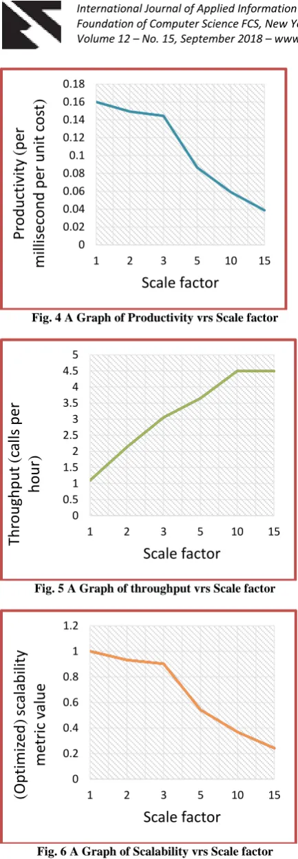
The results of the call processing system as scaled by the metric and same tabulated shows that, the scalability metric values plotted in Fig. 4 drops to 0.8 at the scale factor which is about k = 4. This indicate that the system is scalable up to scale factor of 4. The graph of throughput Verses scale factor in Fig. 5 shows the throughput with a knee at about k = 3 and at this point it has been increased from about 1.08 million calls per hour to about 3.4 million per hour whiles at the same time maintaining good quality of service (QoS). For scale factors (k) beyond 3, the optimization gives a response time which is a little higher than the target value. This is encouraged by the metric, because it also gives a higher throughput. The results of the table and that of the graph plotted in Fig. 4 also shows that the available productivity of the system drops gradually up to k = 3 and from there very sharply. In summary, the results indicate that the scalability is reasonable up to the scale factor of 3 and beyond that, the scalability metric degrades, even though the capacity continues to increase up to about the scale factor of 10. Beyond this factor, the system is bottlenecked and at the same time capacity is saturated. Fig. 6 also shows the graph of scalability against scale factor.
Table 4 Scalability Metric Results for the Call Processing System (*The response time is normalized to the target mean response time of 10min.) Scale
factor
Optical No. of replica Productivity (Optimized) (ms -1
per unit cost)
Scalability metric value (Optimized)
Throughput (Calls per hour) x 106
Normalized* Response Time
System Cost (units) Database Location
server
1 1 1 0.1600 1 1.0958 0.72 1.1
2 1 1 0.1492 0.9325 2.1273 0.88 2.1
3 1 6 0.1444 0.9025 3.0531 0.89 3.1
5 4 2 0.0866 0.5415 3.6485 1.16 5.4
10 2 4 0.0589 0.3683 4.4934 1.11 10.2
15 2 10 0.0387 0.2421 4.4934 1.12 15.2
0 0.2 0.4 0.6 0.8 1 1.2 1.4 1.6
0 1 2 3 4 5 6 7
Rule
o
f
th
u
mb
sc
alab
ilit
y
b
o
u
n
d
Scale factor
1 1.0335 0.9726 0.8986
0.8264 0.7602
0.7006
0 0.2 0.4 0.6 0.8 1 1.2
0 1 2 3 4 5 6
sc
al
abi
lity
me
tr
ic
va
lue
Fig. 4 A Graph of Productivity vrs Scale factor
Fig. 5 A Graph of throughput vrs Scale factor
Fig. 6 A Graph of Scalability vrs Scale factor
5.
CONCLUSION AND
RECOMMENDATIONS
The metric derived in this paper is a strategy based scalability metric that generalizes the well-known metrics for scalability of parallel computations to describe heterogeneous distributed systems. It is worthy to note that, in these systems, a uniform increase in all components types is ideally not a reasonable scaling strategy. What makes this derived metric unique is the fact that, it separates the impact of throughput and response
time on the metric, formalizing the notation of a scaling strategy, introducing QoS evaluation and more also, introducing formal scalability enablers which are optimized at each scale factor. The derived metric is the ratio of the system’s productivity in a scaled version to the productivity of a base case. It also gives a reasonable results for a large collection of idealized and well understood systems nodes which is in the form of queueing modes suitable for distributed systems unlike the other metric like fixed size speedup, where the scaling strategy is to use k processors, throughput is the inverse of completion time, cost is k and quality of service function is given as F = 1. More also, the scalability that deals with fixed time speedup also deals with the use of k processors, but it changes the workload (W) to a value which keeps the completion time constant. In that strategy, throughput is constant, cost is k and quality of service function is F = W.
In the case of call processing system, it can be concluded that the call processing system is scalable up to the scale factor of 4 and at that level, it is capable of supporting roughly 3.3 million calls per hour. If it becomes necessary to scale further than this, then recommendations would be as followsː
1. The software objects organization into concurrent tasks ought to be redesigned in order to make their execution and communication demands more equal. 2. Modification of the database schema can be triedin
order to partition the database in various domains instead of replicating it and also, the consistency management overheads can be reduced.
6.
REFERENCES
[1] Amdahl G. M., Validity of the Single Processor Approach to achieving Large Scale Computing Capabilityties. In Proceedings of the AFIPS Spring Joint Computer Conference, pages 483–485, April1967 [2] Gustafson J. L., Montry G. R., and Benner R. E.
Development of Parallel Methods for a 1024-node Hypercube. SIAM Journal on Scientific and Statistical Computing, 9(4):609–638, 1988
[3] Sun X-H. and Gustafson J. L. Towards a better Parallel Performance Metric. ParallelComputing, 17:1093– 1109,1991
[4] Karp A. H. and Flatt H. P. Measuring Parallel processor Performance. Communications of the ACM, 33(5):539– 543, May 1990.
[5] Kumar V. and Rao V. N. Parallel Depth-First Search.
International Journalof Parallel Programming,
16(6):501–519, 1987
[6] Kung H. T. The Structure of Parallel Algorithms.
Advances in Computers, 19:65–112, 1980. Edited by Marshall C. Yovits and Published by Academic Press, New York.
[7] Jamieson L. H, Gannon D. B., and Douglas R. J., The Characteristics of Parallel Algorithms, pages 65–100. MIT Press, 1987.
[8] Agarwal A. Limits on Interconnection Network Performance. IEEE Transactions on Parallel and Distributed Systems, 2(4):398–412, October 1991.
0 0.02 0.04 0.06 0.08 0.1 0.12 0.14 0.16 0.18
1 2 3 5 10 15
Pr
o
d
u
ct
ivit
y
(
p
er
millisec
o
n
d
p
er
u
n
it
c
o
st
)
Scale factor
0 0.5 1 1.5 2 2.5 3 3.5 4 4.5 5
1 2 3 5 10 15
Th
ro
u
gh
p
u
t
(
calls
p
er
h
o
u
r
)
Scale factor
0 0.2 0.4 0.6 0.8 1 1.2
1 2 3 5 10 15
(
O
p
timiz
ed
)
sc
alab
ility
me
tric
valu
e
[9] Pfister G. F. and Norton V. A. Hot Spot Contention and Combining in Multistage Interconnection Networks.
IEEE Transactions on Computer Systems, C-34(10):943– 948, October 1985.
[10]Anderson T. E. The Performance of Spin Lock Alternatives for Shared-Memory Multiprocessors. IEEE Transactions on Paralleland Distributed Systems, 1(1):6–16, January 1990.
[11]Mellor-Crummey J. M. and Scott M. L. Algorithms for Scalable Synchronization on Shared-Memory Multiprocessors. ACM Transactions on Computer Systems, 9(1):21–65, February 1991
[12]Eggers S. J. and Katz R. H. The Effect of Sharing on the Cache and Bus Performance of Parallel Programs. In
Proceedings of the Third International Conference on Architectural Support for Programming Languages and
Operating Systems, pages 257–270, Boston,
Massachusetts, April 1989.
[13]Chen D, Su H, and Yew P. The Impact of Synchronization and Granularity on Parallel Systems. In
Proceedings of the 17th AnnualInternational Symposium on Computer Architecture, pages 239–248, 1990. [14]Cypher R., Ho A., Konstantinidou S., and Messina P.
Architectural requirements of parallel scientific applications with explicit communication. In
Proceedings of the 20th AnnualInternational Symposium on Computer Architecture, pages 2–13, May 1993 [15]Rothberg E, J. Singh P, and Gupta A. Working sets,
cache sizes and node granularity issues for large-scale
multiprocessors. In Proceedings of the 20th
AnnualInternational Symposium on Computer
Architecture, pages 14–25, May 1993."Generic Functional Architectures for Transport Networks," Int'l Telecommunications Union Recommendation no. G. 805, Nov.1995
[16]Crovella M. E. and LeBlanc T. J. Parallel Performance Prediction Using Lost Cycles Analysis. In Proceedings of Supercomputing ’94, November 1994.
[17]Sivasubramaniam A, Singla A, Ramachandran U, and Venkateswaran H. An Approach to Scalability Study of Shared Memory Parallel Systems. In Proceedings of the ACM SIGMETRICS 1994 Conference on Measurement and Modeling of Computer Systems, pages 171–180, May 1994.
[18]Jogalekar P.P. and Woodside C.M., "A Scalability Metric for Distributed Computing Applications in Telecommunications," Proc. 15th Int'l Teletraffic Congress Teletraffic Contributions to the Information Age, pp. 101-110, 1997.
[19]Trantafiliou P. and Taylor D. J, "The Location-Based Paradigm for Replication: Achieving Efficiency and Availability in Distributed Systems, " IEEE Trans. Software Eng., vol. 21, pp. 1-18, Jan. 1995.