Performance Analysis of Hierarchical
Clustering Algorithm
K.Ranjini
Department of Computer Science and Engineering, Einstein College of Engineering, Tirunelveli, India [email protected]
Dr.N.Rajalingam
Department of Management Studies, Manonmaniam Sundaranar University, Tirunelveli, India [email protected]
---ABSTRACT---
Clustering is the classification of objects into different groups, or more precisely, the partitioning of a data set into subsets (clusters), so that the data in each subset (ideally) share some common trait - often proximity according to some defined distance measure. Data clustering is a common technique for statistical data analysis, which is used in many fields, including machine learning, data mining, pattern recognition, image analysis and bioinformatics. This paper explains the implementation of agglomerative and divisive clustering algorithms applied on various types of data. The details of the victims of Tsunami in Thailand during the year 2004, was taken as the test data. Visual programming is used for implementation and running time of the algorithms using different linkages (agglomerative) to different types of data are taken for analysis.
Keywords: Agglomerative, Divisive, Clustering, Tsunami Database, Data mining
--- Date of Submission: March 10, 2011 Date of Acceptance: May 03, 2011 --- 1. Introduction
D
ata mining is the process of analyzing data from different perspectives and summarizing it into useful information. Technically, data mining is the process of finding correlations or patterns among dozens of fields in large relational databases. Extraction of hidden predictive information from large databases is a powerful new technology in data mining, which has a great potential to help companies to focus on the most important information in their data warehouses. They scour databases for hidden patterns, finding predictive information that experts may miss because it lies outside their expectations. Data mining tools predict future trends and behaviors, allowing businesses to make proactive, knowledge-driven decisions. The automated, prospective analyses offered by data mining move beyond the analyses of past events provided by retrospective tools typical of decision support systems. Data mining tools can answer business questions that traditionally were too time-consuming to resolve. [1][2][14]Data mining commonly involves four classes of tasks:
• Association rule learning – Searches for relationships between variables.
• Clustering – is the task of discovering groups and structures in the data that are "similar" in
some way or another, without using known structures in the data.
• Classification – is the task of generalizing known structure to apply to new data.
• Regression – Attempts to find a function which models the data with the least error. [3]
Among the technique used clustering is the most important and widely used technique. Cluster analysis or clustering is the assignment of a set of observations into subsets (called clusters) so that observations in the same cluster are similar in some sense. It is a method of unsupervised learning, and a common technique for statistical data analysis used in many fields, including machine learning, data mining, pattern recognition, image analysis, information retrieval, and bioinformatics.
Clustering methods are divided into hierarchical and partitioning clustering. Hierarchical algorithms find successive clusters using previously established clusters. These algorithms usually are either agglomerative ("bottom-up") or divisive ("top-down"). Agglomerative algorithms begin with each element as a separate cluster and merge them into successively larger clusters. Divisive algorithms begin with the whole set and proceed to divide it into successively smaller clusters. [4]
dissimilarity/similarity between sets of observations is required. In most methods of hierarchical clustering, this is achieved by use of an appropriate metric (a measure of distance between pairs of observations), and a linkage criterion which specifies the dissimilarity of sets as a function of the pairwise distances of observations in the sets. The results of hierarchical clustering are usually presented in a dendrogram. [5]. The choice of an appropriate metric will influence the shape of the clusters, as some elements may be close to one another according to one distance and farther away according to another.
1.1 Linkage criteria
The linkage criterion determines the distance between sets of observations as a function of the pair wise distances between observations. Some of the commonly used linkage criteria are Single Linkage, Complete Linkage, and Average Linkage.
In this paper, agglomerative and divisive hierarchical clustering algorithms with three linkages are implemented using Visual programming. The algorithms are tested against Tsunami Victim database. Database of the people who were affected by Tsunami during the year 2004, in and around Thailand is taken for testing. The database is selected as it has different types of fields such as numeric, string, and binary.
2. Distance measure
Cluster analysis discovers the natural groupings of the items (or variables). To measure the association between objects a quantitative scale is developed. These scales are referred as similarity measures and are mainly statistical measures that indicate the distances between each of the objects.[16]
2.1 Distance measures for numeric data
Different distance measures give different relative distance between given elements. Selecting a distance measure that determines how the similarity of two elements is an important step in any clustering.
Euclidean distance, Minkowski distance, Manhattan (City-Block), etc., are well known methods used for clustering Numericfield. However, all distance measures yields the same result for 1-norm distance. So,
Euclidean Method is selected for this research. 2.1.1 Euclidean distance
Euclidean distances are usually computed from raw data, and not from standardized data. This method has certain advantages (e.g., the distance between any two objects is not affected by the addition of new objects to the analysis, which may be outliers). However, the distances can be greatly affected by differences in scale among the dimensions from which the distances are computed. For example, if one of the dimensions denotes a measured length in centimeters, and you then convert it to millimeters (by multiplying the values by 10), the
resulting Euclidean or squared Euclidean distances (computed from multiple dimensions) can be greatly affected, and consequently, the results of cluster analyses may be very different.
This is the most commonly chosen type of distance. It simply is the geometric distance in the multidimensional space. [6][12][13]
The Euclidean distance between points P=(p1,p2,…pn)and Q = (q1,q2,…qn), is calculated using:
!"#$%& '%() *
%+,
… … … ….#1(
Where, p i is the data point in x-axis
Where, q i is the data point in y-axis
2.2 Distance measures for binary data
Pairs of items are often compared on the basis of the presence and absence of certain characteristics, when there exists no meaningful p - dimensional measurements. Similar items have more characteristics in common than dissimilar items. The presence or absence of certain characteristics is described mathematically by introducing a binary variable (0 or 1), 1 for the presence of the characteristic and 0 for the absence of the characteristic.
The bit strings that characterize two objects may also be used to calculate a "distance." This effective distance may then be used with a clustering algorithm to place the objects into groups.
Given two objects, A and B, each with n binary attributes, each attribute of A and B can either be 0 or 1. The total number of each combination of attributes for both A and B are specified as follows:
• M11 represents the total number of attributes where
A and B both have a value of 1.
• M01 represents the total number of attributes where
the attribute of A is 0 and the attribute of B is 1. • M10 represents the total number of attributes where
the attribute of A is 1 and the attribute of B is 0. • M00 represents the total number of attributes where
A and B both have a value of 0. Some other symbols that will be used are
• Mi (= M10 + M11) is the total number of ON bits in
object A.
• Mj (= M01 + M11) is the total number of ON bits in
object B.
• MC (= M11) is the total number of times a bit is ON
in both bit strings.
• MI (= M00 + M11) is the total number of times the
two bit strings agree.
• L (= M00 + M01 + M10 + M11) is the length of the bit
string.
Simple Matching - Sokal & Michener, Russel & Rao, Tanamoto Coefficient etc are the commonly used similarity metrics. In this paper, Simple Matching Sokal & Michener distance measure is used for clustering
Simple Matching - Sokal & Michener is calculated using the formula:
SM = MI/L …... (2)
2.3
Distance
measures for string dataString metrics (also known as similarity metrics) are a class of textual based metrics resulting in a similarity or dissimilarity (distance) score between two pairs of strings for approximate matching or comparison.
Hamming Distance and Levenshtein Distance are the well known methods used for string fields.
Levenshtein Distance is chosen for clustering as Hamming distance has a constraint that the string must be of equal length.
2.3.1 Levenshtein Distance (LD)
The Levenshtein distance (LD) is a measure of the similarity between two strings which is defined as the minimum number of edits needed to transform one string into the other, with the allowable edit operations being insertion, deletion, or substitution of a single character. If we refer the source string as s and the target string as t, the distance is the number of deletions, insertions, or substitutions required to transform s into t. For example,
• If s is "test" and t is "test", then LD(s,t) = 0, because no transformations are needed. The strings are already identical.
• If s is "test" and t is "tent", then LD(s,t) = 1, because one substitution (change "s" to "n") is sufficient to transform s into t.
The greater the Levenshtein distance, the more different the strings are. [10]
3. Hierarchical agglomerative algorithms Given a set of N items to be clustered, and an N*N distance (or similarity) matrix, the basic process of hierarchical clustering is this:
a.Start with N clusters, and a single sample indicates one cluster.
b.Find the closest (most similar) pair of clusters and merge them into a single cluster, so that it has one cluster less.
c.Compute distances (similarities) between the new cluster and each of the old clusters.
d.Repeat steps 2 and 3 until all items are clustered into a single cluster of size N. [7][15][19]
The distances between each pair of clusters are computed to choose two clusters that have more opportunity to merge. There are several ways to calculate the distances between the clusters. Methods for measuring association between clusters are called linkage methods.
Linkage Methods or Measuring Association d12
Between Clusters 1 and 2 [18]
• Single Linkage method - cluster objects based on the minimum distance between them (also called the nearest neighbor rule)
/,)0 4%*%3/#1%,2%( … … … #3(
• Complete Linkage method - cluster objects based on the maximum distance between them (also called the furthest neighbor rule)
/,)0 456%3/#1%,2%( … … … #4(
• Average Linkage method - cluster objects based on the average distance between all pairs of objects (one member of the pair must be from a different cluster) [9]
/,)0 1
78 " " /91%,23:
;
3+, <
%+,
… … ….#5(
4. Hierarchical divisive algorithms
Divisive algorithms begin with one cluster that includes all data and start splitting. The single cluster splits into 2 or more clusters based on higher dissimilarity between them. Splitting continues till the number of clusters becomes equal to the number of samples or as specified by the user, whichever is less. The following algorithm is a kind of divisive algorithms that adopts splinter party method.[21][22]
4.1 Divisive algorithm
a.Initially start with a single cluster encompassing all elements;
b.Select l, the largest cluster or the cluster with highest diameter;
c.Find the element e in l that has the lowest average similarity to the other elements in l;
d.e is the first element added to the splinter group while the other elements in l remain in the original group;
e.Find the element f in the original group that has highest average similarity with the splinter group; f.If the average similarity of f with the splinter group
is higher than its average similarity with the original group then assign f to the splinter group and go to Step 5; otherwise do nothing;
g.Repeat Step 2 – Step 6 until each element belong to its own cluster. [8]
5. Implementation
In this paper the agglomerative clustering algorithm with different linkages and divisive algorithm are implemented using Visual Programming and their performance are compared for all the basic data types and for various numbers of records.
As the researcher wish to implement the algorithm using all the three basic data types; numeric, string and binary, this Tsunami Database that contains 8000 records having all data types is used for the study.[11][20][23]
5.1 Tsunami database structure
Table 1:Tsunami Database
S.No Field Name Type
1. Id Numeric
2. Record Number Numeric
3. Name Character
4. Age Numeric
5. Sex Binary
6. Nationality Character
7. Province Character 8. Injured / Dead Binary
5.2 Implementation of Hierarchical Clustering Algorithm Hierarchical algorithms may be applied for different
types of data fields like Character or String Field, Numeric Field and Binary Field.
This database contains three numeric fields, Id, Record number, and Age. As the user need to select the field based on which the database has to be clustered. As Id and Record number are unique fields and they cannot be clustered. The database may be clustered only with the Age field.
6. Performance analysis of the algorithms Analysis is made for the performance which is based on the running time needed to execute agglomerative and divisive algorithm. The nature of the field and the number of records were been taken for analyzing the performance.
From the database, one field for each type of data i.e. sex field for binary data type, age field for numeric type and province field for string data type are taken for comparison In addition, two fields are combined together and the performance of the algorithm is compared as a special category with Sex and Injured/Dead.
6.1 Performance of hierarchical clustering algorithms in clustering different natures of field
Hierarchical clustering algorithms are applied for clustering the database using different natures of data field - binary, numerical, and string variables and based on the combination of two (binary) fields and the respective times are noted for the analysis.
6.1.1 Clustering using agglomerative - single linkage clustering algorithm
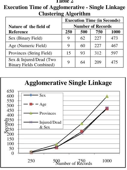
Table 2 shows the execution times of agglomerative - single linkage clustering algorithm in clustering the database based on different natures of data fields – binary, numeric, string, etc. and for varied number of records.
Table 2
Execution Time of Agglomerative - Single Linkage Clustering Algorithm
Nature of the field of Reference
Execution Time (in Seconds) Number of Records 250 500 750 1000
Sex (Binary Field) 9 62 227 473
Age (Numeric Field) 9 60 227 467
Provinces (String Field) 15 93 312 597
Sex & Injured/Dead (Two
Binary Fields Combined) 9 64 209 475
Figure 1: Execution Time of Agglomerative - Single Linkage Clustering Algorithm
It is shown from fig. 1 that the execution time for clustering the database using agglomerative – single linkage algorithm is comparatively high for clustering based on the string variable. When clustering based on binary, numeric and combination of two binary fields the algorithm require almost equal time. The execution time increases with the increase in the size of the database. 6.1.2 Clustering Using Agglomerative – Complete Linkage Clustering Algorithm
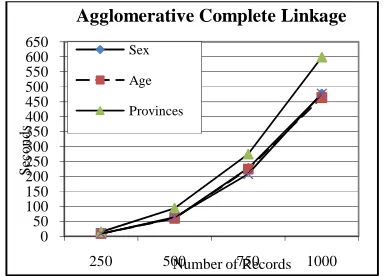
Table 3 shows the execution times of agglomerative - complete linkage clustering algorithm in clustering the database based on different natures of data field – binary, numeric, string, etc. and for varied number of records.
Table 3
Execution Time of Agglomerative – Complete Linkage Clustering Algorithm
Nature of the field of Reference
Execution Time (in
S )
Number of Records 250 500 750 1000
Sex (Binary Field) 9 62 228 476
Age (Numeric Field) 9 60 225 464
Provinces (String Field) 15 94 275 599
Sex & Injured/Dead (Two
Binary Fields Combined) 9 64 208 477
0 50 100 150 200 250 300 350 400 450 500 550 600 650
250 500 750 1000
S
ec
onds
Number of Records
Agglomerative Single Linkage
Sex
Age
Provinces
Figure 2: Execution Time of Agglomerative – Complete Linkage Clustering Algorithm
It is seen from fig. 2 that the execution time for clustering the database using agglomerative –complete linkage algorithm is comparatively high for clustering based on the string variable. When clustering based on binary, numeric and combination of two binary fields the algorithm require almost equal time. The execution time increases with the increase in the size of the database. 6.1.3 Clustering Using Agglomerative – Average Linkage Clustering Algorithm
Table 4
Execution Time of Agglomerative – Average Linkage Clustering Algorithm
Nature of the field of Reference
Execution Time (in Number of Records
250 50
0 750 100
0
Sex (Binary Field) 9 62 229 471 Age (Numeric Field) 8 60 228 464 Provinces (String
Field) 15 93 312 600
Sex & Injured/Dead (Two Binary Fields Combined)
10 64 209 477
Table 4 shows the execution times of agglomerative – average linkage clustering algorithm in clustering the database based on different natures of data field – binary, numeric, string, etc. and for varied number of records.
It is seen from fig. 3 that agglomerative – average linkage algorithm also shows the same time requirement pattern for clustering the database using different natures of fields as exhibited in single and complete linkage agglomerative algorithms.
Figure 3: Execution Time of Agglomerative – Average Linkage Clustering Algorithm
6.1.4 Clustering Using Divisive Clustering Algorithm Table 5 shows the execution times of divisive clustering algorithm in clustering the database based on different natures of data field – binary, numeric, string, etc. and for varied number of records.
Table 5
Execution Time of Divisive Clustering Algorithm
Nature of the field of Reference
Execution Time (in Seconds)
Number of Records
250 500 750 1000
Sex (Binary Field) 8 65 162 363
Age (Numeric Field) 3 9 20 38
Provinces (String Field) 12 52 112 215
Injured/Dead & Sex (Two Binary Fields Combined)
5 36 107 262
Figure 4: Execution Time of Divisive Clustering Algorithm
It is seen from fig. 4 that divisive clustering algorithm requires comparatively very less time to cluster the database using the numeric field. Differing from other clustering algorithms, divisive algorithm requires comparatively more time for binary field than the string field. Also divisive algorithm requires lesser time to cluster when two binary fields are combined to form the base for the clusters.
0 50 100 150 200 250 300 350 400 450 500 550 600 650
250 500 750 1000
S
ec
o
nds
Number of Records Agglomerative Complete Linkage
Sex
Age
Provinces
0 50 100 150 200 250 300 350 400 450 500 550 600 650
250 500 750 1000
S
ec
o
nds
Number of Records Agglomerative Average Linkage
Sex
Age
Provinces
0 50 100 150 200 250 300 350 400 450 500 550 600 650
250 500 750 1000
Seco
n
d
s
Number of Records
Divisive Clustering
Sex
Age
7. Conclusion
This paper analyzes the performance of agglomerative and divisive algorithm for various data types.
From this work it is found that the divisive algorithm works as twice as fast as that of agglomerative algorithm. It is also found that the time needed for string data type is high when compared to the other. The next observation is, in the case of binary field, the time needed to execute a two combined binary field is slightly larger or less equal to the time needed for single binary field. It is also found that the running time get increased on an average of 6 times when the number of records get doubled. More over the running time for all the agglomerative algorithms for same type of data and for same amount of records is more or less equal.
References
1. “Data Mining: What is Data Mining?” in www.anderson.ucla.edu/faculty/jason.frand/teacher/tech nologies/palace/datamining.htm
2. “An Introduction to Data Mining” in www.thearling.com /text/dmwhite/dmwhite.htm
3. Fayyad, Usama, Gregory Piatetsky-Shapiro, and Padhraic Smyth, From Data Mining to Knowledge Discovery in Databases, American Association for Artificial Intelligence- AI Magazine, FALL 1996, 37-54 4. “Types of clustering” in http://en.wikipedia.org/wiki/ Hierarchical
5. “Cluster analysis” in http://en.wikipedia.org/wiki/ Cluster analysis
6. “Hierarchical clustering” in http://hierarchical-clustering .co.tv/
7. “A Tutorial on Clustering Algorithms” in http://home.dei.
polimi.it/matteucc/Clustering/tutorial_html/hierarchical. html
8. Maria Irene Miranda: “Clustering methods and algorithms”
http://www.cse.iitb.ac.in/dbms/Data/Courses/CS632/199 9/clustering/dbms.htm
9. Sheppard, A. G. (1996). The sequence of factor analysis and cluster analysis: Differences in segmentation and dimensionality through the use of raw and factor scores. Tourism Analysis, 1(Inaugural Volume), 49-57.
10. “Levenshtein distance” in www.merriampark.com/ld.htm
11.“Tsunami victim list“ http://www.ems.narenthorn. thaigov. net/tsunami_e/tsunamilist.php
12. Auffarth, B. (2010). Clustering by a Genetic Algorithm with Biased Mutation Operator. WCCI CEC.
IEEE, July 18–23, 2010. http://citeseerx.ist.psu.edu/viewdoc/summary?doi=10.1.1
.170.869
13. Ines Färber, Stephan Günnemann, Hans-Peter Kriegel, Peer Kröger, Emmanuel Müller, Erich Schubert, Thomas Seidl, Arthur Zimek (2010). "On Using Class-Labels in Evaluation of Clusterings". In Xiaoli Z. Fern, Ian Davidson, Jennifer Dy. MultiClust: Discovering,
Summarizing, and Using Multiple Clusterings.ACM.SIGKDD.http://eecs.oregonstate.edu/r
esearch/multiclust/Evaluation-4.pdf
14. Osmar R. Zaïane: “Principles of Knowledge Discovery in Databases - Chapter 8: Data Clustering” http://www.cs.ualberta.ca/~zaiane/courses/cmput690/slid es/Chapter8/index.html
15. Stephen P. Borgatti: “How to explain hierarchical clustering”
http://www.analytictech.com/networks/hiclus.htm 16. H. Finch, Comparison of distance measures in cluster analysis with dichotomous data. Journal of Data Science, 3, 2005, 85-100
17. Margaret H. Dunham, Data mining introductory and advance topics, Low price Edition – Pearson Education, Delhi, 2003.
18. K.P.Soman, Shyam Diwakar, and V.Ajay, Insight into data mining- theory and practice, Eastern Economy Edition, Prentice Hall of India Pvt. Ltd, New Delhi, 2006 19. Sung Young Jung, and Taek-Soo Kim, An Agglomerative Hierarchical Clustering Using Partial Maximum Array and Incremental Similarity Computation Method, Proceedings of the 2001 IEEE International Conference on Data Mining, November 29-December 02, 2001, 265-272.
20. R.J.Gil-Garcia and J.M.Badia-Contelles, A General Framework for Agglomerative Hierarchical Clustering Algorithms A Pons-Porrata Pattern Recognition, ICPR 2006. 18th International Conference 2, 2006, 569 – 572 21. Hui-Chuan Lin (2009) Survey and Implementation of Clustering Algorithms, Master’s thesis, Hsinchu, Taiwan, Republic of China
22. Jiawei Han and Micheline Kamber, Data Mining Concepts and Techniques, Second Edition- Morgan Kaufmann Publishers, San Francisco, 2006.
23. Evangelos Petroutsos, “Mastering Visual Basic 6”, BPP publications, New Delhi.
AUTHORS’ BIOGRAPHY
K. Ranjini got her M.Sc., (Comp. Sci.) degree from Madurai Kamaraj University. Further she got M.Tech and M.Phil degrees. She has a teaching experience of Seven years. She is interested in data mining and attempting to find novel applications of data mining concepts.