C O R R E S P O N D E N C E
Open Access
Quantification of population benefit in evaluation
of biomarkers: practical implications for disease
detection and prevention
Xiaohong Li
1,2*, Patricia L Blount
1,3, Brian J Reid
1,2,3,5and Thomas L Vaughan
1,4Abstract
Background:With the rapid development of“-omic”technologies, an increasing number of purported biomarkers have been identified for cancer and other diseases. The process of identifying those that are most promising and validating them for use at the population level for prevention and early detection is a critical next step in achieving significant health benefits.
Methods:In this paper, we propose that in order to effectively translate biomarkers for practical clinical use, it is important to distinguish and quantify the differences between the use of biomarkers and other risk factors to identify preventive interventions versus their use in disease risk prediction and early detection. We developed mathematical models for quantitatively evaluating risk and benefit in use of biomarkers for disease prevention or early detection. Simple numerical examples were used to demonstrate the potential applications of the models for various types of data. Results:We propose an index which takes into account potential adverse consequences of biomarker-driven interventions–the‘naïve’ratio of population benefit (RPB)–to facilitate evaluating the potential impact of biomarkers on cancer prevention and personalized medicine. The index RPB is developed for both binary and continuous biomarkers/risk factors. Examples with computational analyses are presented in the paper to contrast the differences in using biomarkers/risk factors for prevention and early detection.
Conclusions:Integrating epidemiologic knowledge into clinical decision making is a key step to translate new biomarkers/risk factors into practical use to achieve health benefits. The RPB proposed in this paper considers the absolute risk of a disease in intervention, and takes into account the risk-benefit effects simultaneously for a marker/exposure at the population level. The RPB illustrates a unique approach to quantitatively assess the risk and potential benefits of using a biomarker/risk factor for intervention in both early detection and prevention.
Keywords:Ratio of population benefit, RPB, Biomarkers, Disease prevention, Disease early detection, Clinical decision making, Biomarkers for early detection, Risk/benefit analysis
Background
The identification of robust cancer risk factors and biomarkers are the cornerstones of modern approaches to cancer prevention and personalized medicine. A large number of environmental and host risk factors (either inherited or somatic) have been identified that are associated with cancer risk, and with rapidly-advancing
“-omics”technologies, the reported number of biomarkers proposed for clinical use is increasing dramatically. How-ever, the translation of these for use in the population or clinic in such a way as to have a significant impact on can-cer incidence and mortality is still a major challenge. The process of selecting and evaluating the most promising biomarkers for clinical application among the large number of purported biomarkers is a critical step in the translation process. Key to this process is distinguishing the differences between evaluating biomarkers and risk factors for primary prevention programs versus disease risk prediction and
* Correspondence:[email protected] 1
Divisions of Public Health Sciences, Fred Hutchinson Cancer Research Center, 1100 Fairview Ave. N., Seattle, WA 98109, USA
2
Human Biology, Fred Hutchinson Cancer Research Center, 1100 Fairview Ave. N., Seattle, WA 98109, USA
Full list of author information is available at the end of the article
© 2014 Li et al.; licensee BioMed Central Ltd. This is an Open Access article distributed under the terms of the Creative Commons Attribution License (http://creativecommons.org/licenses/by/2.0), which permits unrestricted use, distribution, and reproduction in any medium, provided the original work is properly credited. The Creative Commons Public Domain Dedication waiver (http://creativecommons.org/publicdomain/zero/1.0/) applies to the data made available in this article, unless otherwise stated.
early detection. Quantitative analysis of these differences can facilitate the translational process.
Pepe et al. [1] compared the association of a marker with a disease, often quantified in case-control or cross-sectional studies by the odds ratio (OR), with use of the marker for disease classification (i.e. presence or absence of cancer in a sample), and illustrated the limitation of the OR in gauging the performance of a diagnostic, prognostic, or screening marker. More recently, the use of markers discovered in genetic association studies for disease risk prediction was specifically addressed by Jakobsdottir et al. [2]. The limitations of using markers for medical diagnosis or early detection also have been comprehensively assessed [3-5]. Recently, an increasing number of studies have focused on the use of previously-identified risk factors and biomarkers (e.g., one or more constitutive SNPs (single-nucleotide polymorphism)) for cancer prevention or for pathway-targeted therapy develop-ment [6,7]. In practice, the specific criteria for evaluating a biomarker or risk factor for disease detection/prediction could be quite different than that for disease prevention. To highlight and evaluate these differences quantitatively, we first illustrate the numerical relationship between the OR of a biomarker/risk factor and its population attribut-able risk percent (PAR%) (assuming causality) in the con-text of a population prevention program. We then illustrate the corresponding accuracy, as measured by sensitivity and specificity, for a biomarker/risk factor with identical charac-teristics (OR and prevalence) in the context of a disease detection/prediction program. Finally we propose an index–the‘naïve’ratio of population benefit (RPB)–for quantifying overall risk/benefit of using a biomarker for cancer prevention or detection/prediction at the popula-tion level. Analyses are presented separately for binary and continuous biomarkers.
Methods and results
Numerical relationships between sensitivity, specificity and population attributable risk for binary and continuous biomarkers
Calculation for binary marker/risk factor
The PAR% is often used to estimate the fraction of the total disease burden in the population that would not have occurred if a causal risk factor were absent [8]. To help introduce the latter parts of the paper, we first illustrate the numerical relationships between PAR% for causal binary markers/risk factors at different prevalence and relative risk levels and the corresponding sensitivity and specificity of using a marker/risk factor with identi-cal characteristics for disease classification/prediction (Table 1). The status of a specific binary risk factor (e.g. a mutated gene or exposure) and the observed disease outcome status, also binary, can be displayed as a stand-ard 2 × 2 contingency table, with the four cells labeled
a(+/+), b(+/-), c(-/+) and d(-/-) corresponding to the counts of individuals in a cohort with status of exposure and outcome (+ for yes, - for no), respectively. If out-come is directly predicted by the marker, for calculation of sensitivity and specificity (either for screening or screening-based disease intervention), the data can be arranged in an identical 2 × 2 table with the individual cells labeled a (true positive), b (false positive), c (false negative) and d (true negative) relating the biomarker status with a true outcome status or“gold standard”.
Using the counts in the four cells of the contingency table (whether corresponding to exposure and outcome or disease classification) several commonly used quan-tities can be obtained. A binary marker/risk factor has two possible values, leading to fixed sensitivity (a/(a + c)) and specificity (d/(b + d)) values in a population with a specific OR and marker prevalence, in which the inci-dences in exposed (or marker carriers) and unexposed (or marker non-carriers) are a/(a + b), c/(c + d) respectively. Table 1 shows the numerical relationships among i) preva-lence of a risk factor/marker, ii) the relative risk of disease associated with the marker (indicated by OR), iii) PAR%, iv) sensitivity, and v) specificity. If we let r1= ((a + c)/(a + b + c + d)),r2=c/(c + d), (r1is the prevalence andr2is the false negative fraction), the population attributable risk can be calculated as PAR% = (r1 - r2)/r1100%. By definition, the false positive fraction = 1-specificity; the false negative fraction = 1-sensitivity; and the OR = (sensitivity/(1-sensitivity))/((1-specificity)/specificity). In Table 1, ma-rker prevalence and risk factor exposure prevalence are interchangeable algebraically; the former used for early detection and risk prediction, and the later used for preven-tion. The calculation of PAR% above was based on the assumption of no adjustment for potential confounders. A common way to obtain PAR% adjusted for confounders is to use a stratification approach: PARadj%¼
X
i
piPARi%
wherepiis the proportion of cases in stratum i, PARi% is the PAR% estimated from stratum i. More details for dealing with confounders can be found in Rothman
et al. [9].
Numerical analysis for continuous marker/risk factor
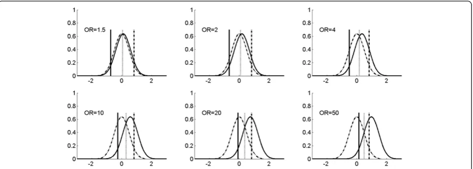
Pepe et al. [1] evaluated the limitation of the OR in gauging the performance of a diagnostic, prognostic, or screening marker. Illustrated here is the use of continu-ous biomarkers both for diagnostic/prognostic/screening and for prevention, along with the relationship between the OR value and PAR% parameters for the continuous markers. Figure 1 presents a few hypothetical normal distributions of continuous markers/risk factors with dif-ferent OR risk values.
For the continuous distribution markers, the sensi-tivity and specificity can be calculated as follows [10],
Liet al. BMC Medical Informatics and Decision Making2014,14:15 Page 2 of 12
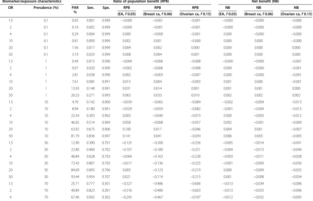
Table 1 Numerical illustration for calculating RPB of hypothetical binary markers using data of three cancers as examples
Biomarker/exposure characteristics Ratio of population benefit (RPB) Net benefit (NB)
OR Prevalence (%) PAR
%
Sen. Spe. RPB RPB RPB NB NB NB
(EA,f0.03) (Breast ca,f0.06) (Ovarian ca,f0.15) (EA,f0.03) (Breast ca,f0.06) (Ovarian ca,f0.15)
1.5 0.1 0.05 0.001 0.999 −0.000 −0.001 −0.001 −0.000 −0.000 −0.000
2 0.1 0.10 0.002 0.999 −0.000 −0.001 −0.001 −0.000 −0.000 −0.000
4 0.1 0.29 0.004 0.999 0.000 −0.000 −0.001 0.000 −0.000 −0.000
10 0.1 0.81 0.009 0.999 0.002 0.001 −0.000 0.000 0.000 −0.000
20 0.1 1.56 0.017 0.999 0.004 0.002 0.000 0.000 0.000 0.000
50 0.1 3.19 0.033 0.999 0.008 0.004 0.001 0.000 0.000 0.000
1.5 1 0.49 0.015 0.990 −0.004 −0.006 −0.008 −0.000 −0.000 −0.001
2 1 0.97 0.020 0.990 −0.002 −0.006 −0.008 0.000 −0.000 −0.001
4 1 2.81 0.038 0.990 0.002 −0.003 −0.007 0.000 −0.000 −0.001
10 1 7.61 0.085 0.991 0.015 0.004 −0.003 0.001 0.000 −0.001
20 1 13.93 0.148 0.991 0.031 0.014 0.001 0.001 0.001 0.000
50 1 26.33 0.271 0.993 0.063 0.033 0.010 0.002 0.002 0.002
1.5 10 4.70 0.142 0.900 −0.039 −0.065 −0.084 −0.002 −0.004 −0.013
2 10 8.94 0.180 0.901 −0.029 −0.059 −0.082 −0.001 −0.004 −0.013
4 10 22.54 0.303 0.902 0.003 −0.040 −0.073 0.000 −0.003 −0.012
10 10 46.05 0.514 0.904 0.058 −0.008 −0.057 0.002 −0.001 −0.009
20 10 63.92 0.675 0.906 0.100 0.017 −0.046 0.004 0.001 −0.007
50 10 81.79 0.836 0.907 0.141 0.041 −0.034 0.006 0.003 −0.005
1.5 30 12.90 0.390 0.701 −0.125 −0.200 −0.256 −0.005 −0.014 −0.041
2 30 22.80 0.460 0.702 −0.107 −0.189 −0.251 −0.004 −0.013 −0.040
4 30 46.84 0.628 0.703 −0.064 −0.163 −0.238 −0.003 −0.011 −0.038
10 30 72.43 0.807 0.705 −0.017 −0.136 −0.225 −0.001 −0.009 −0.036
20 30 84.69 0.893 0.706 0.005 −0.123 −0.219 0.000 −0.009 −0.035
50 30 93.44 0.954 0.707 0.021 −0.114 −0.215 0.001 −0.008 −0.034
1.5 70 25.71 0.777 0.301 −0.327 −0.486 −0.606 −0.013 −0.034 −0.096
2 70 40.89 0.823 0.301 −0.316 −0.480 −0.603 −0.013 −0.033 −0.096
4 70 67.46 0.902 0.302 −0.295 −0.467 −0.597 −0.012 −0.032 −0.095
Li
et
al.
BMC
Medical
Informatic
s
and
Decision
Making
2014,
14
:15
Page
3
o
f
1
2
http://ww
w.biomedce
ntral.com/1
Table 1 Numerical illustration for calculating RPB of hypothetical binary markers using data of three cancers as examples(Continued)
10 70 86.14 0.958 0.303 −0.280 −0.459 −0.593 −0.011 −0.032 −0.094
20 70 92.92 0.979 0.303 −0.275 −0.456 −0.591 −0.011 −0.032 −0.094
50 70 97.13 0.991 0.303 −0.272 −0.454 −0.591 −0.011 −0.031 −0.094
ca= cancer. EA= esophageal adenocarcinoma. f= loss adjustment factor of quality-adjusted life year. NB= net benefit. OR= odds ratio.
The table shows numerical relationship between Odds ratio, Marker prevalence, PAR% of binary markers and their RPB based on the cancer data of three studies. NB were also calculated.
The table assumes 1% disease prevalence in general population. For PAR%, sensitivity and specificity similar patterns are observed with other disease prevalence values less than about 10%. Disease prevalence affects RPB more directly (see text).
Li
et
al.
BMC
Medical
Informatic
s
and
Decision
Making
2014,
14
:15
Page
4
o
f
1
2
http://ww
w.biomedce
ntral.com/1
Sensitivity¼P Yð D>cÞ ¼Φ μDσD−c
; Specificity¼1−PYD>c
¼
1−Φ μD−c σD
, where D indicates non-disease group, andc
is the threshold above which a positive (disease) call will be made. In contrast to binary markers, which only have one set of sensitivity and specificity values, con-tinuous markers can be used to generate infinite sets of sensitivity and specificity values depending on the threshold value ofc.
To quantify PAR% for continuous markers, letwbe the proportion of diseased individuals in a population or risk of a disease in the general population, then for a marker with a continuous value, a specific set of sensitivity and specifi-city is obtained for a given threshold c, the risk of ‘ unex-posed’(the proportion of subjects, either diseased or non-diseased whose marker level is lower than the thresholdc)
que with threshold c can be calculated as que¼
w½1−R∞
cfdð Þxdx 1−w
ð ÞRc
−∞fdð Þxdxþw½1−
R∞ cfdð Þxdx
¼
wð1−sensitivitycÞ 1−wð Þspecificitycþwð1−sensitivitycÞ ,
where fd(x) and fd xð Þ are the probability density dis-tribution of a biomarker in the diseased and non-diseased group respectively (assuming normal distribu-tion),sensitivitycandspecificitycare the sensitivity and specificity of the continuous marker at threshold c. Therefore, for a continuous marker, we have PAR% = (w–que)/w. Table 2 shows the numerical relationships
among sensitivity and specificity and PAR% of the quantification for various thresholdscin Figure 2.
Distinguishing the use of biomarkers/risk factors for cancer detection and prevention
Above we presented the numerical relationships between sensitivity, specificity and PAR% for binary and continu-ous biomarkers (Tables 1 and 2). Below we use examples to illustrate the importance of distinguishing between the use of biomarkers for cancer detection/risk predic-tion and for cancer prevenpredic-tion since the consequences of false positive and false negative findings may differ substantially in these two contexts.
Example 1: Genotype and bladder cancer. A genetic association study [11] showed strong evidence that the copy number of gene GSTM1 is significantly associated with risk of bladder cancer, with an OR = 1.9 corre-sponding to the GSTM1 null genotype (51% prevalence). If this marker were used as a binary marker for bladder cancer detection in the general population, it would result in 66% sensitivity and 50% specificity, a poor marker for diagnostic purposes. However, if a drug were to be developed that targeted the pathway(s) by which GSTM1 null increases risk, and if the drug were 100% effective in preventing bladder cancer without toxic side effects (and ignoring costs), then treatment of all marker carriers would reduce bladder cancer by 31% (PAR%),
Figure 1Hypothetical distribution patterns of continuous markers with different relative risks, and thresholds for risk prediction. Two normal distributions (mean = 0 and standard deviation = 0.5) are used to represent the distribution of a continuous marker in disease (solid curved line) and non-disease (dashed curved line) populations for six different ORs. The locations of the means for the disease population are consistent with the logit modelPr(D =1|X) =α+βX, in which one unit increase corresponds to the OR shown in the figure. The three vertical bars (solid, dotted, and dashed) correspond to different thresholds (cut off value‘c’) for positive-negative calls of a disease with a continuous distribution marker. Specifically, the solid bar represents the threshold valuecsuch that the sensitivity is kept for 0.95 for various OR values in the plot; the dotted bar represents the threshold valuecsuch that the sensitivity and specificity are equal for various OR values in the plots; and the dashed bar represents the threshold valuecsuch that the specificity is kept for 0.95 for various OR values in the plot. The examples of using the continuous marker for disease classification or prevention are shown in Figure 2; and corresponding sensitivity, specificity and PAR% of various thresholds (three bars in this Figure) are shown in Table 2 and Figure 2 (the cross, circle, and triangle in Figure 2 correspond to solid, dashed, and solid vertical bars in Figure 1).
Liet al. BMC Medical Informatics and Decision Making2014,14:15 Page 5 of 12
which would represent a substantial public health bene-fit. One way to quantify such a benefit can be performed using the method developed in this paper as shown in example 4.
Example 2: Smoking and lung cancer.Using Table 1, if the prevalence of smoking (risk factor) in a population is 30%, and the OR of smoking for lung cancer risk is esti-mated to be 10- to 20-fold higher than the non-smokers, then the corresponding PAR% value is 73-85% (had all smokers not smoked, there would have been 73% to 85% fewer lung cancers). The corresponding false positive fraction is about 29.3%, which indicates among the non-lung cancer group (normal), 29.3% are smokers. This high ‘false positive’ fraction may be tolerable for lung cancer prevention since reducing 73-85% of lung cancers at the ‘expense’ of abstaining from smoking is likely ac-ceptable. (If other diseases caused by smoking are con-sidered, this argument is even stronger). Quantification
of such benefit can be accomplished using the method developed in this paper as shown in example 3.
Quantitative evaluation of the benefit of using
biomarkers for disease detection/prediction and disease prevention at the population level
The above numerical analyses and specific examples indi-cate that traditional measures of association (OR, PAR%, sensitivity, specificity, and others) can have dramatically dif-ferent implications depending on whether they are applied to risk prediction, early detection or prevention of disease. Since false positive and false negative classifications are un-avoidable in practice [12], we propose an index, the‘naïve’ ratio of population benefit (RPB), which takes into account the adverse effects of misclassification, for evaluating the impact of using biomarkers for early detection/risk predic-tion and preventive intervenpredic-tions on a disease at the popu-lation level. Unlike OR, PAR%, sensitivity, specificity, and
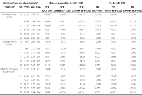
Table 2 Numerical illustration for calculating RPB of hypothetical continuous markers using data of three cancers as examples
Biomarker/exposure characteristicsa Ratio of population benefit (RPB) Net benefit (NB)
(Threshold)b OR PAR% Sen. Spe. RPB RPB RPB NB NB NB
(EA, f 0.03) (Breast ca, f 0.06) (Ovarian ca, f=0.15) (EA, f=0.03) (Breast ca, f=0.06) (Ovarian ca, f=0.15)
Fixed sensitivity (95%)
1.5 33.22 0.95 0.07 −0.456 −0.659 −0.812 −0.018 −0.046 −0.129
2 48.88 0.95 0.09 −0.440 −0.641 −0.792 −0.017 −0.045 −0.126
4 71.30 0.95 0.16 −0.389 −0.583 −0.728 −0.015 −0.040 −0.115
10 84.46 0.95 0.29 −0.287 −0.466 −0.601 −0.011 −0.032 −0.095
20 89.01 0.95 0.43 −0.187 −0.352 −0.475 −0.007 −0.024 −0.075
50 92.25 0.95 0.61 −0.051 −0.196 −0.305 −0.002 −0.014 −0.048
Fixed specificity (95%)
1.5 2.59 0.08 0.95 −0.019 −0.032 −0.043 −0.001 −0.002 −0.007
2 4.95 0.10 0.95 −0.013 −0.029 −0.041 −0.001 −0.002 −0.007
4 12.67 0.17 0.95 0.006 −0.018 −0.036 0.000 −0.001 −0.006
10 27.40 0.31 0.95 0.041 0.002 −0.028 0.002 0.000 −0.004
20 41.15 0.44 0.95 0.074 0.021 −0.019 0.003 0.001 −0.003
50 60.16 0.62 0.95 0.119 0.047 −0.008 0.005 0.003 −0.001
Balanced sensitivity & specificityc
1.5 14.83 0.54 0.54 −0.208 −0.316 −0.397 −0.008 −0.022 −0.063
2 23.89 0.57 0.57 −0.178 −0.285 −0.366 −0.007 −0.020 −0.058
4 42.57 0.64 0.63 −0.114 −0.222 −0.304 −0.005 −0.015 −0.048
10 60.28 0.72 0.72 −0.030 −0.137 −0.218 −0.001 −0.010 −0.035
20 70.68 0.78 0.77 0.024 −0.085 −0.166 0.001 −0.006 −0.026
50 80.17 0.84 0.84 0.088 −0.020 −0.101 0.003 −0.001 −0.016
Numerical relationships between Odds ratio and PAR% of continuous markers and their RPB based on the data of three studies. ca= cancer. EA= esophageal adenocarcinoma. f = loss-adjustment factor of quality-adjusted life year. NB= net benefit. OR= odds ratio. Sen.= sensitivity, Spe.= specificity.
The disease prevalence of population used for the table = 0.01. As shown in the formula of RPB for continuous markers, disease prevalence w will directly affect the value of RPB.
a
Hypothetical continuous biomarker/exposure with assumed distributions as described in Figure1.
b
Threshold used for continuous biomarkers positive are the thresholds shown in Figure1(three vertical bars).
c
Using a threshold that lead to sensitivity and specificity closest to the upper left corner of ROC curve coordinates for cutoff.
Liet al. BMC Medical Informatics and Decision Making2014,14:15 Page 6 of 12
other similar measures which do not directly depend on disease prevalence, the RPB does account for disease preva-lence in a reasonable way as shown in the following parts of the paper. This new index is not intended for evaluating or comparing the prediction accuracy of biomarkers or pre-diction models; instead it is intended for analyzing the po-tential benefit for a population using a previously-selected biomarker for disease intervention after taking into account potential adverse effects.
RPB for binary markers/risk factors
Using the 2 × 2 contingency table introduced earlier, if no biomarker is used for early cancer detection/cancer risk prediction, lethal cancer cases will occur (a+c); with a subset of individuals (b+d ) remaining cancer free. The quantification of lives lost in this situation is−f1∗(a+c), and lives gained isf2∗(b+d), with the negative sign in-dicating loss; (−f1 represents naïve quantification of lives lost due to cancer cases discovered at a late incur-able stage), a positive value,f1represents lives gained if cancer is detected early, andf2represents naïve quanti-fication of lives gained due to non-cancer subjects who are not classified as cancer (gain due to perfect markers with no false positives and−f2represents loss due to a false positive call). If a binary biomarker is used for cancer detection, then letabe the cancer cases that will be detected earlier (true positive), andbbe the number of non-cancer cases are classified as cancer due to false positives associated with this biomarker. The sum of
gains and losses associated with this biomarker is f1a+ (−f1c) + (−f2b) +f2d. Note, the sum of losses and gains associated with not using the biomarker −f1(a+c) +f2 (b+d); hence, the change of total net gain for compari-son using a biomarker vs. no biomarker isf1a−f2b,(no change for −f1c+f2d when comparing the two sums, assuming false negative callscwill be treated the same as no biomarker). For a population, if all cancer cases could be detected early without false positives (an ideal marker), the sum of gains and losses for the population is f1∗(a+c) +f2∗(b+d). Therefore, assuming binary biomarkers for cancer detection are not perfect (with false positives and false negatives), a naïve estimation of the ratio of population benefit (RPB) can be
esti-mated by RPB¼ f1a−f2b f1ðaþcÞþf2ðbþdÞ
¼
af1−bf2 af1þbf2þcf1þdf2 . Note that changes in disease prevalence are accounted for in the RPB calculation, which uses all of the terms defining prevalence (a + c)/(a + b + c + d). The RPB is different from Net Benefit (NB) based on decision curve analysis [13,14]. NB =(a−wb)/(a + b + c + d),
where w is the weight for counting the cost of false positive relatives to the cost of false negatives. The de-nominator of NB counts the cost of the overall popula-tion, whereas the denominator of RPB only counts the cost for worst possible performance of a marker i.e. the counts for true positiveaand true negativedboth are 0 in prediction. In addition, RPB also considers adverse effect (δ) due to intervention as shown in the next section. There-fore, RPB is more sensitive in evaluating false positive or false negative costs compare to NB. The adjusted RPB for potential confounders can also be obtained by the weighted average of individual RPB for each strata in stratified analysis, a similar idea to the adjusted PAR% mentioned above [9]. RPBadj¼
X
i
pi aif1i−bif2i
aif1iþbif2iþcif1iþdif2i
,
wherepiis the proportion of cases in stratumi, andai,
bi, ci, di, f1i, and f2i are same as in RPB above but are
estimated from specific stratumi.RPB is a percentage of net gain, which is a ratio of net gains in the group of marker carriers (or risk factor exposed), including diseased and non-diseased, against overall gain esti-mated by quantifying the losses and gains due to false positive, false negative, true positive and true negative. Disease prevalence is considered in RPB calculation.
For cancer prevention with consideration of adverse effects (i.e. prevention measure is applied to the carriers of a predictive (or risk-causal) biomarker or those
ex-posed to a risk factor), the RPB¼ aηf1−aδ−bδ af1þbf2þcf1þdf2, similarly, f1and f2are defined as the same as the binary marker mentioned above; ηrepresents the efficacy of a prevention measure (i.e. the percentage of cancer re-duced due to a prevention measure); and δ represents
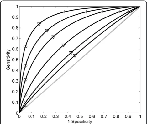
Figure 2Disease prediction performance evaluated by ROC curves for the hypothetical continuous markers with different relative risks.ROC curves for continuous risk marker with different odds ratios (from bottom to top OR = 1.5, 2, 4, 10, 20, 50), which corresponding to the distribution plots of continuous markers shown in Figure 1. The crosses correspond to a fixed sensitivities; the circles to a fixed specificities; and triangles to equal sensitivities and specificities. Their corresponding PAR% values are shown in Table 2.
Liet al. BMC Medical Informatics and Decision Making2014,14:15 Page 7 of 12
possible adverse effect of a prevention measure (i.e. side ef-fect of a drug for cancer prevention). When there is no ad-verse effect from a prevention measure,δ= 0. Numerically, RPB could be negative, 0 or positive, which indicates detri-mental, neutral, or beneficial overall effects at the popula-tion level, respectively. In addipopula-tion, the absolute gain for early cancer detection or cancer prevention may be quanti-fied as (af1- bf2)–h(a + b), and (aηf1- aδ- bδ)–h(a + b) respectively, wherehis the coefficient for the cost of preven-tion or treatment of exposed subjects or subjects positive for specific markers. Following are two examples illustrat-ing the use of RPB for binary markers and risk factors.
Example 3: Smoking and lung cancer. Since there are no negative health effects due to abstaining from smok-ing, we set δ= 0, and RPB becomes aηf1/(af1+ bf2+ cf1+ df2), where η in the example represents efficacy (%) of lung cancer reduction due to abstaining from smoking.
Example 4: Genotype and bladder cancer. GSTM1 is a bladder cancer associated biomarker (marker prevalence = 51%, OR = 1.9). If a drug were developed that targeted the effect associated with the null GSTM1 variant, and if all carriers of the risk variant were treated with the drug, the drug had no adverse side effects and is 100% effective (δ= 0,
η= 1), then RPB =af1/(af1+ bf2+ cf1+ df2). However, if the efficacy of a drugηis much less than 1 and/or the drug has adverse effects (δ> 0), then RPB will be smaller or even could become negative. In practice, properly quantifying f1 andf2may be very complex. However, if the analyses of the efficacy of the drug for cancer prevention and early detec-tion are only limited to the diseased group (ignorebandd
andf1≠0) then RPB is equal to the marker’s sensitivity multi-plied byðηf1−δÞ
f1
.
Example 5: CNV and neuroblastoma. A copy number
variation associated with neuroblastoma was reported re-cently [15]. The prevalence of the marker (1q21.1) in the general population is about 9%, and the OR of the marker (copy loss) for neuroblastoma risk is estimated to be around 3. If this marker were dichotomized as a binary marker for predicting the absence or presence of the disease, it will result in a 23% sensitivity and 91% specificity, with a PAR% of approximately 15%, which indicates the marker could account for about 15% of neuroblastoma risk if the disease is truly caused by the CNV (copy-number variation). As-sume a drug is developed that targeted this marker (1q21.1) for prevention. If the drug is 100% effective in disease pre-vention and had no side effects and all persons who were carriers for the marker were treated with the drug, it would reduce the total disease cases by 15% (PAR%). However, in the more likely scenario, drugs have significant side effects and are not 100% effective such that more extensive risk benefit analyses are needed. The RPB proposed in this paper could be used for quantifying and evaluating the feasibility for population intervention in such a case.
Example 6: RPB calculation for three cancers for bin-ary markers or risk factors. The utility weights for quality-adjusted life years have been estimated for surgi-cal treatment of esophageal adenocarcinoma [16], breast cancer [17], and ovarian cancer [18]; these are 0.97; 0.94; and 0.85 respectively. The corresponding adjustment factors for loss of quality of life (f2) are 0.03, 0.06, and 0.15 respectively for the three cancers. If a cancer were detected early and intervention were a complete success, this would lead to a benefit value of 1 (true positive detected early); if a subject were wrongly diagnosed with cancer and surgery was done, the cost value can be repre-sented as the loss adjustment factor for quality-adjusted life year. This leads us to havef1= 1,f2= loss-adjustment factor of a disease intervention to calculate RPB proposed above. Using breast cancer as an example,f2= 0.06, since RPB¼ af1−bf2
af1þbf2þcf1þdf2¼
a1−b0:06
a1þb0:06þc1þd0:06, where a, b, c, and d are the number of true positive, false positive, false negative, and true negative due to using a biomarker for disease outcome prediction for intervention. In many cases, the OR has been estimated for a marker or risk fac-tors. In Table 1, we show the relationship among RPB and various ORs and prevalence of a marker or risk factor using the loss-adjustment factors of the three cancers as examples. We also calculated net benefit (NB) values under these scenarios for comparison. For instance, from Table 1, if a biomarker has 1% prevalence with OR 10 for breast cancer risk, then the RPB = 0.004, if OR = 20, RPB = 0.014. If a biomarker has 10% prevalence with OR 10, then the RPB = -0.008; if OR = 20, RPB = 0.017. It will be possible to apply these principles to other diseases, novel risk assess-ments and new treatassess-ments as additional data become available. Table 1 shows numerical examples with the as-sumption of 1% disease prevalence. Disease prevalence of a population will directly affect RPB as the aand c
in the 2×2 table are used in the calculation of RPB. For instance, if disease prevalence is changed from 1% to 3%, and assuming a biomarker (or exposure) preva-lence of 30%, the RPB for a risk biomarker with various OR values 1.5, 2, 4, 10, 20, and 50 will be: 0.05, 0.086, 0.172, 0.266, 0.311, 0.345 respectively for EA; -0.064, -0.04, 0.02, 0.084, 0.116, 0.139 respectively for breast cancer; and -0.18, -0.167, -0.134, -0.099, -0.082, -0.069 respect-ively for ovarian cancer.
RPB for continuous markers and risk factors
For a continuous marker, the ‘naïve’ ratio of popula-tion benefit for early cancer detecpopula-tion (present or absent) or prevention can be calculated as RPB¼
wf1 R∞
cfdð Þxdx−ð1−wÞf2
R∞ cfdð Þxdx
wf1 R∞
cfdð Þxdxþð1−wÞf2
R∞
cfdð Þxdxþwf1 Rc
−∞fdð Þxdxþð1−wÞf2 Rc
−∞fdð Þxdx
,
wherewis disease prevalence in a population,fd(x) and
fdð Þx are the probability density distribution of a
Liet al. BMC Medical Informatics and Decision Making2014,14:15 Page 8 of 12
biomarker in the diseased and the non-diseased group re-spectively and c is the cutoff threshold for positive and negative calls for a continuous marker. This formula can also be modified to address potential confounding factors using stratified analysis. The adjusted RPB for a con-founding factor of a continuous marker is: RPBadj¼
P
i
pi
wif1i
R∞
cfd ið Þxdx−ð1−wiÞf2i
R∞ cfd ið Þxdx
wif1i
R∞
cfdið Þxdxþð1−wiÞf2i
R∞
cfd ið Þxdxþwif1i
Rc
−∞fdið Þxdxþð1−wiÞf2i
Rc
−∞fd ið Þxdx
,
where pi is the proportion of cases in stratum i, and the quantification for loss f1i, and f2i are the same as in RPB
above but are estimated in specific stratum i.The density distribution functions fdi(x) and fd ið Þx are the density
distributions of a biomarker in the disease and the non-disease group respectively in stratum i.Similar to binary markers, the ‘naïve’ ratio of population benefit for cancer prevention using continuous markers with consider-ation of adverse effects could be calculated as RPB¼
wf1 R∞
cηð Þxfdð Þxdx−w
R∞
cδð Þxfdð Þxdx−ð1−wÞ
R∞ cδð Þxfdð Þxdx
wf1 R∞
cfdð Þxdxþð1−wÞf2
R∞
cfdð Þxdxþwf1
Rc
−∞fdð Þxdxþð1−wÞf2 Rc
−∞fdð Þxdx
,
whereη(x) is efficacy (as a function of x) of a prevention measure andδ(x)represents adverse effect due to a preven-tion measure. Similar calculapreven-tions can be used to obtain RPB ifδ(x)andη(x)are dependent onfd(x) andfdð Þx .The total lives gained for early cancer detection and cancer pre-vention using a continuous marker may be quantified as
wf1R∞cfdð Þxdx−ð1−wÞf2R∞cfdð Þx dx
−h w R∞cfdð Þx dxþ
1−w
ð ÞR∞cfdð Þx dxÞ, and wf1R∞cηð Þx fdð Þx dx−wRc∞δ ð Þxfd x
ð Þdx−ð1− wÞ R∞cδð Þx fdð Þx dxÞ−h w R∞cfdð Þx dxþ ð1− wÞ
R∞
cfdð Þx dxÞ, respectively. As defined for binary markers
above,h is the coefficient for quantification of the cost of prevention or treatment for exposed subjects or subjects with positive markers; the other parameters remain the same as defined for binary markers. For example, BMI (body mass index) is a continuous marker [19]; studies have shown the association between high BMI and esophageal adenocarcinoma risk [20-22]. If this is a causal association, then BMI may not be a robust marker for detecting presence or absence of disease. However, if BMI were considered as a modifiable risk factor, then false positives may be tolerable since redu-cing BMI for those people who would never develop esophageal adenocarcinoma had their BMI not been re-duced will likely not have substantial detrimental effects (δ= 0, RPB always >0). If we use BMI≥30 as the threshold
c and assumed no negative effect (δ= 0) for reducing BMI for those who have a BMI ≥30, then the RPB¼
wf1 R∞
cηð Þxfdð Þxdx
wf1 R∞
cfdð Þxdxþð1−wÞf2
R∞
cfdð Þxdxþwf1
Rc
−∞fdð Þxdxþð1−wÞf2 Rc
−∞fdð Þxdx
;
whereη(x)is the efficacy of cancer reduction by reducing BMI,fd(x) andfdð Þx are the BMI distribution in a specific at risk population and low risk population, respectively. However, if negative effects occur when reducing BMI
(δ> 0), e.g., if a medication used for weight loss is asso-ciated with significant side effects, then the RPB will be smaller. The RPB, therefore, could be used to quantify the potential overall benefit of a prevention measure targeted to a marker or risk factor. Similar to binary markers, if the analysis of effects for prevention and disease detection is restricted to the diseased group only (ignorefd
x
ð Þ in RPB above) for a continuous marker in prevention, and assuming no negative effect (δ= 0), then the RPB
be-comes R∞
cηð Þxfdð Þxdx
R∞ cfdð Þxdxþ
Rc
−∞fdð Þxdx
, which is an estimation of
pre-vention effects with consideration of at risk subjects only, and it will always have a positive value (benefit).
Example 7: RPB calculation for continuous markers or risk factors. To evaluate the benefit of using a continu-ous biomarker or risk factor for disease intervention, the probability density distribution of the marker in the population of disease outcome fd(x) and non-disease outcome fdð Þx can be estimated from observed popula-tion data. Then, to calculate RPB of the continuous bio-marker, a threshold c of the biomarker is chosen (i.e., any subjects with the biomarker level above the thresh-old will be predicted to have the disease outcome); then numerical integration can be used to obtain RPB for the continuous markers using the formula above. For example, using the same loss of quality of life adjustment factors of the three cancers shown in Example 6 (the loss factorf2are 0.03, 0.06, and 0.15 for the three cancers), assume the prob-ability distributions of a continuous marker in the popula-tion with diseasefd(x) and without diseasefdð Þx follow the normal distributions with different means as shown in Figure 1. Using numerical integration for the RPB formula above, we calculated the RPB for various scenarios in which the hypothetical continuous markers have different OR for the cancer risk as shown in Table 2. In these calculations, the thresholdscof the continuous biomarker were chosen to demonstrate various possibilities for outcome prediction including fixed sensitivity, fixed specificity, and balanced sensitivity and specificity. Table 2 shows numerical exam-ples with assumption of 1% disease prevalence for RPB calculation. Disease prevalence wof a population will dir-ectly affect RPB value. For example, for a breast cancer bio-marker with balanced sensitivity and specificity if the disease prevalence is changed from 1% to 3%, the cor-responding RPB values for a risk biomarker with vari-ous OR values 1.5, 2, 4, 10, 20, and 50 will be changed from -0.316, -0.285,-0.222, -0.137, -0.085, -0.020 for 1% prevalence to -0.12, -0.09, -0.025, 0.058, 0.112, 0.176 respectively for 3% prevalence.
Discussion
With rapid advances in various technologies, a large num-bers of biomarkers have been reported to be associated
Liet al. BMC Medical Informatics and Decision Making2014,14:15 Page 9 of 12
with various diseases, including cancer. Translating those to the clinic and for public health benefit is a critical but difficult next step. For example, genome-wide association studies are identifying hundreds of SNPs associated with a variety of diseases. While the rich discoveries from such studies continue to prompt investigation of pathway-targeted interventions for disease prevention and therapy [6], it is generally believed that use of single or combined SNP information can achieve only modest improvement in disease risk prediction or early detection programs for indi-viduals in the general population as compared to current clinical screening modalities [23-27]. This underscores the need for quantitative evaluation of both the risk and poten-tial benefit of biomarkers since in this process many factors need to be considered including sensitivity and specificity of the marker used for risk prediction or targeted therapy, disease prevalence and quantitative relationship between biomarker levels and meaningful risk measures, cost, and risk/benefit analyses [28-30]. In this paper, we call attention to the need to distinguish and quantify the consequences of false positive and false negative diagnoses of a marker for prevention and early detection/risk prediction. The RPB es-timation can be confounded due to the marker or risk ex-posure. Adjustment for potential confounders in estimating RPB need be considered.
Table 1 shows the numerical relationships between measurements commonly used for cancer detection and prevention. For a marker with a low prevalence, the sen-sitivity of the marker is very low even when it has a high OR value. Combining multiple SNP/CNV markers with low OR values for prediction may have limited effects at the population level, i.e. a person who carries all 10‘risk’ SNPs will be at high risk for the disease; however very few people carry all 10 SNPs in the general population, thus leading to a low PAR% value. Therefore, using such a panel may have a low impact on disease detection or risk prediction in the general population, although it might be applied to the few individuals in that category. Based on three published data sets, the numerical calcu-lations of RPB for the three cancers are presented in Tables 1 and 2. The calculations show that due to low specificity of a marker and the disease intervention ac-tion based on the predicac-tion of the markers in the tables, risk is larger than benefit (RPB < 0) in many cases. How-ever, we used the loss of quality of life adjustment factor from the three cancers in a simple way to demonstrate the application of the RPB. The risk and benefit may be affected by many factors such as age, time, or unknown confounders.
Six phases are recommended for developing effective bio-markers, with longitudinal studies considered essential for validation [31]. Pepeet al. [32] presented a comprehensive method for evaluating the predictiveness of a biomarker and its performance as a disease classifier. The application
of PAR% was evaluated for benefit of community-based ef-forts to prevent disease using a specific cancer marker by Wacholder [33]. Furthermore, the quantitative connection between biomarker levels in cases and controls and clinical meaningful risk measures or testing also has been carefully evaluated by Wentzensen and Wacholder [30], adding a useful tool for apprising candidate biomarkers at an early stage. The RPB proposed in this study takes account of both accuracy of outcome prediction of a marker and bene-fit for a population if the marker were used for an interven-tion. The prediction accuracy of biomarker(s) should be assessed and compared with validated or well-established tools (such as area under the curve, integrated discrimin-ation improvement, net reclassificdiscrimin-ation improvement etc.). Then the value of biomarker(s) should be further evaluated for risk and benefit if it were to be applied in a large popu-lation for intervention. In this paper, we assumed the selec-tion of biomarker(s) for predicselec-tion has been completed, and we propose the RPB for risk and benefit analysis at the population level when a given marker or risk factor is used for disease intervention. Specifically, we concentrate on the framework of risk/benefit analysis in using a marker for dis-ease prevention and detection/prediction.
The 1,000 Genomes Project is expected to discover substantially more SNP markers and other variants that have frequency between 0.5 to 5%. Those data could be analyzed by the methods presented in this paper. Thus far, the performance of SNP/CNV for disease risk pre-diction or risk stratification still needs improvement [34], while their potential for disease prevention or tar-geted therapy [7] and prediction of prognosis [35] is sub-stantially encouraging. A broad risk/benefit analysis will be needed when translating the results of such studies into clinical use for cancer risk prediction, detection and prevention. Greenland [36] pointed out that the eva-luation of marker prediction models are linked to predictor-conditional performance, cut-point choices, and error costs; and there is a need for reorientation toward cost-effective prediction. We extended the issue further by distinguishing between using biomarkers for early disease detection and using them for prevention. The feasibility or value of using biomarkers in the two scenarios could be generalized by risk/benefit analysis, a research direction that has been proposed in previous studies [37,38]. The proposed RBP for binary and con-tinuous markers/exposures can be extended to health economics studies.
particularly pertinent to two of the eight recommenda-tions: (1) “balance the epidemiology research portfolio beyond traditional emphasis on discovery and etiology research to encompass development and evaluation of clinical and population interventions, implementation, dissemination, and outcomes research”; and (2)“support knowledge integration and meta research (systematic re-views, modeling, decision analysis etc.) to identify gaps, inform funding, and to integrate epidemiologic know-ledge into decision making”. The RPB is intended to il-lustrate an approach to assess the risk and potential benefits using a marker/risk factor for intervention in both early detection and prevention. As such, it is a gen-eral framework, and requires a proper estimation of
‘risk/benefit’quantifications (f1andf2) in the RPB model for each disease. Substantial effort may be needed to properly estimate such parameters for a biomarker to properly evaluate the feasibility of using the biomarkers for different scenarios such as early detection, risk pre-diction, and prevention.
Conclusions
Making use of the discovered biomarkers/risk factors from epidemiological and clinical research for clinical decision making is a key step to translate the discoveries into practical use to achieve health benefits. Risk benefit analysis provides crucial information for disease inter-vention decision making. It is worthwhile to distinguish and quantify the differences between the use of bio-markers/risk factors to identify preventive interventions versus their use in disease risk prediction and early de-tection. The RPB proposed in this paper not only con-siders the absolute risk of a disease in intervention, but also takes into account risk-benefit effects simultan-eously for a marker/exposure at the population level. Using concrete examples, we demonstrate that RPB de-veloped in this study is a useful tool for quantitatively assessing the risk and benefits in using a biomarker/risk factor for intervention in both early detection and prevention.
Abbreviations
CNV:(somatic) Copy number variation; OR: Odds ratio; PAR%: Population attributable risk percent; RPB: The‘naïve’Ratio of population benefit; SNP: Single nucleotide polymorphism.
Competing interests
All authors of this paper declare that they have no competing interests.
Authors' contributions
Author XL initiated the prototype of the manuscript in the environment of close working relationships with other co-authors of the manuscript. PLB and BJR provided input from the clinical application point of view. TLV provided input from the epidemiology and population science point of view. All authors were involved in vigorous discussions during the writing of the manuscript. XL performed the computer programming for all numerical calculations. All authors of the manuscript were actively involved in the editing
and finalization of the submitted manuscript. All authors read and approved the final manuscript.
Acknowledgements
This work was supported by the National Cancer Institute at the National Institutes of Health (Grants P01 CA091955, RC1 CA146973, K05 CA124911, R01 CA136725 and R01 CA179949).
We thank Dr. Dennis Chao and Dr. Ying Q Chen of Fred Hutchinson Cancer Research Center for reading and giving comments on the near final version of the manuscript.
Author details 1
Divisions of Public Health Sciences, Fred Hutchinson Cancer Research Center, 1100 Fairview Ave. N., Seattle, WA 98109, USA.2Human Biology, Fred Hutchinson Cancer Research Center, 1100 Fairview Ave. N., Seattle, WA 98109, USA.3Department of Medicine, University of Washington, 1959 NE Pacific Street, Seattle, WA 98195, USA.4Department of Epidemiology, University of Washington, 1959 NE Pacific Street, Seattle, WA 98195, USA. 5
Department of Genome Sciences, University of Washington, 1959 NE Pacific Street, Seattle, WA 98195, USA.
Received: 17 September 2013 Accepted: 18 February 2014 Published: 6 March 2014
References
1. Pepe MS, Janes H, Longton G, Leisenring W, Newcomb P:Limitations of the odds ratio in gauging the performance of a diagnostic, prognostic, or screening marker.Am J Epidemiol2004,9:882–890.
2. Jakobsdottir J, Gorin MB, Conley YP, Ferrell RE, Weeks DE:Interpretation of genetic association studies: markers with replicated highly significant odds ratios may be poor classifiers.PLoS Genet2009,2:e1000337. 3. Boyko EJ, Alderman BW:The use of risk factors in medical diagnosis:
opportunities and cautions.J Clin Epidemiol1990,9:851–858.
4. Roulston JE:Assessment of predictive values of tumor markers.Methods Mol Med2004,97:13–27.
5. Kattan MW:Judging new markers by their ability to improve predictive accuracy.J Natl Cancer Inst2003,9:634–635.
6. Hirschhorn JN:Genomewide association studies–illuminating biologic pathways.N Engl J Med2009,17:1699–1701.
7. Marian AJ:Molecular genetic studies of complex phenotypes.Transl Res
2012,2:64–79.
8. Markush RE:Levin's attributable risk statistic for analytic studies and vital statistics.Am J Epidemiol1977,5:401–406.
9. Rothman KJ, Greenland S, Lash TL:Modern Epidemiologgy.Philadelphia: Lippincott, Williams & Wilkins; 2008.
10. Pepe MS:The Statistical Evaluation of Medical Tests for Classification and Prediction.New York: Oxford University Press; 2003.
11. Garcia-Closas M, Malats N, Silverman D, Dosemeci M, Kogevinas M, Hein DW, Tardon A, Serra C, Carrato A, Garcia-Closas R, Lloreta J, Castano-Vinyals G, Yeager M, Welch R, Chanock S, Chatterjee N, Wacholder S, Samanic C, Tora M, Fernandez F, Real FX, Rothman N:NAT2 slow acetylation, GSTM1 null genotype, and risk of bladder cancer: results from the Spanish Bladder Cancer Study and meta-analyses.Lancet2005,9486:649–659. 12. Li X, Blount PL, Vaughan TL, Reid BJ:Application of biomarkers in cancer
risk management: evaluation from stochastic clonal evolutionary and dynamic system optimization points of view.PLoS Comput Biol2011, 2:e1001087.
13. Steyerberg EW:Clinical Prediction Models: A Practical Approach to Development, Validation, and Updating.New York: Springer; 2009. 14. Steyerberg EW, Vickers AJ, Cook NR, Gerds T, Gonen M, Obuchowski N,
Pencina MJ, Kattan MW:Assessing the performance of prediction models: a framework for traditional and novel measures.Epidemiology2010, 1:128–138.
15. Diskin SJ, Hou C, Glessner JT, Attiyeh EF, Laudenslager M, Bosse K, Cole K, Mosse YP, Wood A, Lynch JE, Pecor K, Diamond M, Winter C, Wang K, Kim C, Geiger EA, McGrady PW, Blakemore AI, London WB, Shaikh TH, Bradfield J, Grant SF, Li H, Devoto M, Rappaport ER, Hakonarson H, Maris JM:Copy number variation at 1q21.1 associated with neuroblastoma.Nature2009, 7249:987–991.
16. Hur C, Nishioka NS, Gazelle GS:Cost-effectiveness of aspirin chemoprevention for Barrett's esophagus.J Natl Cancer Inst2004,4:316–325.
17. Raftery J, Chorozoglou M:Possible net harms of breast cancer screening: updated modelling of Forrest report.BMJ2011:d7627.
18. Greving JP, Vernooij F, Heintz AP, van der Graaf Y, Buskens E:Is centralization of ovarian cancer care warranted? A cost-effectiveness analysis.Gynecol Oncol2009,1:68–74.
19. Flegal KM, Troiano RP:Changes in the distribution of body mass index of adults and children in the US population.Int J Obes Relat Metab Disord
2000,7:807–818.
20. Lindblad M, Rodriguez LA, Lagergren J:Body mass, tobacco and alcohol and risk of esophageal, gastric cardia, and gastric non-cardia adenocarcinoma among men and women in a nested case-control study.Cancer Causes Control
2005,3:285–294.
21. Kubo A, Corley DA:Body mass index and adenocarcinomas of the esophagus or gastric cardia: a systematic review and meta-analysis.Cancer Epidemiol Biomarkers Prev2006,5:872–878.
22. Corley DA, Levin TR, Habel LA, Buffler PA:Barrett's esophagus and medications that relax the lower esophageal sphincter.Am J Gastroenterol2006,5:937–944.
23. Gail MH:Discriminatory accuracy from single-nucleotide polymorphisms in models to predict breast cancer risk.J Natl Cancer Inst2008,14:1037–1041. 24. Goldstein DB:Common genetic variation and human traits.N Engl J Med
2009,17:1696–1698.
25. Couzin-Frankel J:Major heart disease genes prove elusive.Science2010, 5983:1220–1221.
26. Mealiffe ME, Stokowski RP, Rhees BK, Prentice RL, Pettinger M, Hinds DA: Assessment of clinical validity of a breast cancer risk model combining genetic and clinical information.J Natl Cancer Inst2010,21:1618–1627. 27. Wacholder S, Hartge P, Prentice R, Garcia-Closas M, Feigelson HS, Diver WR,
Thun MJ, Cox DG, Hankinson SE, Kraft P, Rosner B, Berg CD, Brinton LA, Lissowska J, Sherman ME, Chlebowski R, Kooperberg C, Jackson RD, Buckman DW, Hui P, Pfeiffer R, Jacobs KB, Thomas GD, Hoover RN, Gail MH, Chanock SJ, Hunter DJ:Performance of common genetic variants in breast-cancer risk models.N Engl J Med2010,11:986–993.
28. Kraft P, Hunter DJ:Genetic risk prediction–are we there yet?N Engl J Med
2009,17:1701–1703.
29. Katsanis SH, Javitt G, Hudson K:Public health. A case study of personalized medicine.Science2008,5872:53–54.
30. Wentzensen N, Wacholder S:From differences in means between cases and controls to risk stratification: a business plan for biomarker development.Cancer Discovery2013,3(2):148–157.
31. Pepe MS, Etzioni R, Feng Z, Potter JD, Thompson ML, Thornquist M, Winget M, Yasui Y:Phases of biomarker development for early detection of cancer.J Natl Cancer Inst2001,14:1054–1061.
32. Pepe MS, Feng Z, Huang Y, Longton G, Prentice R, Thompson IM, Zheng Y: Integrating the predictiveness of a marker with its performance as a classifier.Am J Epidemiol2008,3:362–368.
33. Wacholder S:The impact of a prevention effort on the community. Epidemiology2005,1:1–3.
34. Ioannidis JP, Castaldi P, Evangelou E:A compendium of genome-wide associations for cancer: critical synopsis and reappraisal.J Natl Cancer Inst
2010,12:846–858.
35. Hartman M, Loy EY, Ku CS, Chia KS:Molecular epidemiology and its current clinical use in cancer management.Lancet Oncol2010,4:383–390. 36. Greenland S:The need for reorientation toward cost-effective prediction: comments on 'Evaluating the added predictive ability of a new marker: from area under the ROC curve to reclassification and beyond' by M. J. Pencina et al., Statistics in Medicine.Stat Med2008,2:199–206. doi:10.1002/sim.2929.
37. Ransohoff DF, Khoury MJ:Personal genomics: information can be harmful. Eur J Clin Invest2010,40:64–68.
38. Khoury MJ, Bowen MS, Burke W, Coates RJ, Dowling NF, Evans JP, Reyes M, Pierre JS:Current priorities for public health practice in addressing the role of human genomics in improving population health.Am J Prev Med
2011,40:486–493.
39. Khoury MJ, Freedman AN, Gillanders EM, Harvey CE, Kaefer C, Reid BC, Rogers S, Schully SD, Seminara D, Verma M:Frontiers in cancer epidemiology: a challenge to the Research Community from the
Epidemiology and Genomics Research Program at the National Cancer Institute.Cancer Epidemiol Biomarkers Prev2012,21:999–1001.
40. Khoury MJ, Lam TK, Ioannidis JP, Hartge P, Spitz MR, Buring JE, Chanock SJ, Croyle RT, Goddard KA, Ginsburg GS, Herceg Z, Hiatt RA, Hoover RN, Hunter DJ, Kramer BS, Lauer MS, Meyerhardt JA, Olopade OI, Palmer JR, Sellers TA, Seminara D, Ransohoff DF, Rebbeck TR, Tourassi G, Winn DM, Zauber A, Schully SD:Transforming epidemiology for 21st century medicine and public health.Cancer Epidemiol Biomarkers Prev2013,22:508–516.
doi:10.1186/1472-6947-14-15
Cite this article as:Liet al.:Quantification of population benefit in evaluation of biomarkers: practical implications for disease detection and prevention.BMC Medical Informatics and Decision Making201414:15.
Submit your next manuscript to BioMed Central and take full advantage of:
• Convenient online submission
• Thorough peer review
• No space constraints or color figure charges
• Immediate publication on acceptance
• Inclusion in PubMed, CAS, Scopus and Google Scholar
• Research which is freely available for redistribution
Submit your manuscript at www.biomedcentral.com/submit