S O F T W A R E
Open Access
Metrics for evaluating 3D medical image
segmentation: analysis, selection, and tool
Abdel Aziz Taha
*and Allan Hanbury
Abstract
Background: Medical Image segmentation is an important image processing step. Comparing images to evaluate the quality of segmentation is an essential part of measuring progress in this research area. Some of the challenges in evaluating medical segmentation are: metric selection, the use in the literature of multiple definitions for certain metrics, inefficiency of the metric calculation implementations leading to difficulties with large volumes, and lack of support for fuzzy segmentation by existing metrics.
Result: First we present an overview of 20 evaluation metrics selected based on a comprehensive literature review. For fuzzy segmentation, which shows the level of membership of each voxel to multiple classes, fuzzy definitions of all metrics are provided. We present a discussion about metric properties to provide a guide for selecting evaluation metrics. Finally, we propose an efficient evaluation tool implementing the 20 selected metrics. The tool is optimized to perform efficiently in terms of speed and required memory, also if the image size is extremely large as in the case of whole body MRI or CT volume segmentation. An implementation of this tool is available as an open source project. Conclusion: We propose an efficient evaluation tool for 3D medical image segmentation using 20 evaluation metrics and provide guidelines for selecting a subset of these metrics that is suitable for the data and the segmentation task.
Keywords: Evaluation metrics, Evaluation tool, Medical volume segmentation, Metric selection
Background
Medical 3D image segmentation is an important image processing step in medical image analysis. Segmentation methods with high precision (including high reproducibil-ity) and low bias are a main goal in surgical planning because they directly impact the results, e.g. the detection and monitoring of tumor progress [1–3]. Warfield et al. [4] denoted the clinical importance of better characterization of white matter changes in the brain tissue and showed that particular change patterns in the white matter are associated with some brain diseases. Accurately recogniz-ing the change patterns is of great value for early diagnosis and efficient monitoring of diseases. Therefore, assessing the accuracy and the quality of segmentation algorithms is of great importance.
Medical 3D images are defined on a 3D grid that can have different sizes depending on the body parts imaged and the resolution. The grid size is given as(w×h×d)
*Correspondence: taha@ifs.tuwien.ac.at
TU Wien, Institute of Software Technology and Interactive Systems, Favoritenstrasse 9-11, A-1040, Vienna, Austria
denoting the width, height, and depth of the 3D image. Each 3D point on the grid is called a voxel. Given an anatomic feature, a binary segmentation can be seen as a partition that classifies the voxels of an image according to whether they are part or not of this feature. Examples of anatomic features are white matter, gray matter, lesions of the brain, body organs and tumors. Segmentation eval-uation is the task of comparing two segmentations by measuring the distance or similarity between them, where one is the segmentation to be evaluated and the other is the corresponding ground truth segmentation.
Medical segmentations are often fuzzy meaning that voxels have a grade of membership in [ 0, 1]. This is e.g. the case when the underlying segmentation is the result of averaging different segmentations of the same structure annotated by different annotators. Here, segmentations can be thought of as probabilities of voxels belonging to particular classes. One way of evaluating fuzzy segmen-tations is to threshold the probabilities at a particular value to get binary representations that can be evaluated as crisp segmentations. However, thresholding is just a
workaround that provides a coarse estimation and is not always satisfactory. Furthermore, there is still the chal-lenge of selecting the threshold because the evaluation results depend on the selection. This is the motivation for providing metrics that are capable of comparing fuzzy segmentations without loss of information. Note that there is another common interpretation of fuzzy segmen-tation as partial volume, where the voxel value represents the voxel fraction that belongs to the class. The fuzzy met-ric definitions provided in this paper can be applied for this interpretation as well.
There are different quality aspects in 3D medical image segmentation according to which types of segmentation errors can be defined. Metrics are expected to indicate some or all of these errors, depending on the data and the segmentation task. Based on four basic types of errors (added regions, added background, inside holes and bor-der holes), Shi et al. [5] described four types of image segmentation errors, namely the quantity (number of seg-mented objects), the area of the segseg-mented objects, the contour (degree of boundary match), and the content (existence of inside holes and boundary holes in the seg-mented region). Fenster et al. [6] categorized the require-ments of medical segmentation evaluation into accuracy (the degree to which the segmentation results agree with the ground truth segmentation), the precision as a mea-sure of repeatability, and the efficiency which is mostly related with time. Under the first category (accuracy), they mentioned two quality aspects, namely the delin-eation of the boundary (contour) and the size (volume of the segmented object). The alignment, which denotes the general position of the segmented object, is another qual-ity aspect, which could be of more importance than the size and the contour when the segmented objects are very small.
Metric sensitivities are another challenge in defining metrics. Sensitivity to particular properties could pre-vent the discovery of particular errors or lead to over- or underestimating them. Metrics can be sensitive to out-liers (additional small segmented objects outside the main object), class imbalance (size of the segmented object rel-ative to the background), number of segmented objects, etc. Another type of sensitivity is the inability to correctly deal with agreement caused by chance. This is related to the baseline value of the metric, which should ideally be zero when the segmentation is done at random, indicating no similarity [7].
There is a need for a standard evaluation tool for med-ical image segmentation which standardizes not only the metrics to be used, but also the definition of each metric. To illustrate this importance, Section “Multiple definition of metrics in the literature” shows examples of metrics with more than one definition in the literature leading to different values, but each of them is used under the
same name. In the text retrieval domain, the TREC_EVAL tool1provides a standardization of evaluation that avoids such confusion and misinterpretation and provides a stan-dard reference to compare text retrieval algorithms. The medical imaging domain lacks such a widely applied instrument.
Gerig et al. [8] proposed a tool (Valmet) for evaluation of medical volume segmentation. In this tool only five met-rics are implemented. There are important metmet-rics, like information theoretical metrics as well as some statisti-cal metrics like Mahalanobis distance, and metrics with chance correction like Kappa and adjusted Rand index, that are not implemented in the Valmet evaluation tool. Furthermore, this tool doesn’t provide support for fuzzy segmentation. The ITK Library2provides a software layer that supports medical imaging tasks including segmenta-tion and registrasegmenta-tion. The ITK Library provides evaluasegmenta-tion metrics that are mostly based on distance transform fil-ters [9]. However, this implementation has the following shortcomings: First, the ITK Library doesn’t implement all relevant metrics needed for evaluating medical segmen-tation. Second, since most of the metrics are based on distance transform filters, they are sensitive to increasing volume grid size in terms of speed as well as memory used. One way to reduce this effect is to use the bounding cube (scene) [6, 10], i.e. the smallest cube including both seg-ments, that is to exclude from calculation all background voxels not in the bounding cube. However, there are some shortcomings using the bounding cube, first the bounding cube remains large when the segments are large, far from each other or there are outliers far from the segments; sec-ond, the bounding cube affects the results of metrics that depend on the true negatives. In Section “Testing the effi ciency”, we show that the ITK implementation of relevant metrics fails to compare segmentations larger than a par-ticular grid size. Since very large medical segmentations, like those of whole body volumes, are already common, this is a significant restriction.
This paper makes the following contributions:
• It provides an overview of 20 evaluation metrics for volume segmentation, selected based on a literature review. Cases where inconsistent definitions of the metrics have been used in the literature are identified, and unified definitions are suggested.
• It provides efficient metric calculation algorithms that work optimally with large 3D image segmentations by taking advantage of their nature as dense distributions of voxels. Efficiency is becoming ever more important due the increasing size of segmentations, such as segmentation of whole body volumes.
segmentation to be taken into account in the evaluation.
• It provides metrics generalized for segmentation with multiple labels
• It provides an efficient open source implementation of all 20 metrics that outperforms state-of-the art tools in common cases of medical image
segmentation
The remainder of this paper is organized as follows: Section “Ethics approval” provides the ethics approval. Section “Evaluation Metrics for 3D image segmenta-tion” presents a short literature review of metrics. In Section “Metric definitions and Algorithms”, we present the definition for each identified metric in the literature review as well as the algorithms used to efficiently cal-culate the metric value. We provide in Section “Mul-tiple definition of metrics in the literature” examples of multiple definition of metrics in the literature that leads to confusion and motivates a standard evaluation tool. Section “Implementation” provides details on the tool implementation, i.e. architecture, programming environ-ment, usage as well as the optimization techniques have been used. Experiments performed to test the tool effi-ciency are presented in Section “Testing the effieffi-ciency”. A discussion about metric properties, bias, and utilities as well as guidelines for metric selection is presented in Section “Metric selection”. We conclude the paper in Section “Conclusion” and give information about the availability and requirements in Section “Availability and requirements”.
Ethics approval
The images used for this study are brain tumor MRI images and segmentations provided by the BRATS2012 benchmark organized in conjunction with the MICCAI 2012 conference, and whole body MRI/CT scans, pro-vided by the VISCERAL project (www.visceral.eu) that were acquired in the years 2004–2008, where data sets of children (< 18 years) were not included due to the recommendation of the local ethical committee number S-465/2012, approval date February 21st, 2013.
Evaluation metrics for 3D image segmentation
We present a set of metrics for validating 3D image seg-mentation that were selected based on a literature review of papers in which 3D medical image segmentations are evaluated. Only metrics with at least two references of use are considered. An overview of these metrics is available in Table 1. Depending on the relations between the met-rics, their nature and their definition, we group them into six categories, namely overlap based, volume based, pair-counting based, information theoretic based, probabilistic based, and spatial distance based. The aim of this grouping
is to first ease discussing the metrics in this paper and second to enable a reasonable selection when a subset of metrics is to be used, i.e. selecting metrics from different groups to avoid biased results.
Metric definitions and Algorithms
We present the definitions of all metrics that have been implemented. Let a medical volume be represented by the point setX = {x1,. . .,xn}with |X| = w×h×d = n wherew,handdare the width, height and depth of the grid on which the volume is defined. Let the ground truth segmentation be represented by the partitionSg= {S1g,S2g} ofXwith the assignment functionfi
g(x)that provides the membership of the objectxin the subsetSig, wherefgi(x)= 1 ifx ∈ Sgi,fgi(x) = 0 ifx ∈/ Sgi, andfgi(x) ∈ (0, 1)if x has a fuzzy membership inSig, i.e.fgi(x)can be seen as the probability ofxbeing inSgi. Furthermore, let the segmen-tation, being evaluated, be represented by the partition St =
S1t,S2t of X with the assignment function ftj(x) that provides the membership ofxin the classSjt, defined analogously to fgi. Note that in this paper, we only deal with partitions with two classes, namely the class of inter-est (anatomy or feature) and the background. We always assume that the first class
S1g,S1t
is the class of
inter-est and the second classS2 g,S2t
is the background. The
assignment functionsfgi andftj can either be crisp when their range is{0, 1} or fuzzy when their range is [ 0, 1]. Note that the crisp partition is just a special case of the fuzzy partition. We also assume that the memberships of a given point xalways sum to one over all classes. This implies that f1
g(x)+ fg2(x) = 1 andft1(x)+ft2(x) = 1 for allx ∈ X. In the remainder of this section, we define the foundation of methods and algorithms used to com-pute all the metrics presented in Table 1. We structure the discussion in this section to follow the metric grouping given in the column “category”. This provides a structure that is advantageous for the implementation of the evalu-ation tool, that is to improve the efficiency by making use of the synergy between the metrics in each group to avoid repeated calculation of the same parameters.
Spatial overlap based metrics
Table 1Overview of the metrics implemented in this tool
Metric Symb. Reference of use in medical images cat. Definition
Dice (=F1-Measure) DICE [1, 2, 15, 16, 57–63] 1 (6)
Jaccard index JAC [15, 16, 21–23, 59, 60, 62] 1 (7)
True positive rate (Sensitivity, Recall) TPR [10, 16, 60, 62–64] 1 (10)
True negative rate (Specificity) TNR [10, 16, 60, 62] 1 (11)
False positive rate (=1-Specificity, Fallout) FPR →Specificity 1 (12)
False negative rate (=1-Sensitivity) FNR →Sensitivity 1 (13)
F-Measure (F1-Measure=Dice) FMS →Dice 1 (15), (16)
Global Consistency Error GCE [21–23, 65, 66] 1 (17) to (19)
Volumetric Similarity VS [15, 21–23, 59, 61, 67] 2 (21)
Rand Index RI [21, 22, 65, 66] 3 (30)
Adjusted Rand Index ARI [68, 69] 3 (32)
Mutual Information MI [2, 32, 57] 4 (33) to (38)
Variation of Information VOI [21, 22, 65, 66] 4 (39), (35)
Interclass correlation ICC [8, 70] 5 (41)
Probabilistic Distance PBD [8, 59] 5 (43)
Cohens kappa KAP [1, 62] 5 (44) to (46)
Area under ROC curve AUC [2, 64, 69] 5 (47)
Hausdorff distance HD [8, 15, 59, 61–63, 71, 72] 6 (48), (49)
Average distance AVD [62, 63] 6 (50), (51)
Mahalanobis Distance MHD [15, 73] 6 (52) to (54)
The symbols in the second column are used to denote the metrics throughout the paper. The column “reference of use” shows papers where the corresponding metric has been used in the evaluation of medical volume segmentation. The column “category” assigns each metric to one of the following categories: (1) Overlap based, (2) Volume based, (3) Pair counting based, (4) Information theoretic based, (5) Probabilistic based, and (6) Spatial distance based. The column “definition” shows the equation numbers where the metric is defined
Basic cardinalities For two crisp partitions (segmenta-tions)SgandSt, the confusion matrix consists of the four common cardinalities that reflect the overlap between the two partitions, namelyTP,FP,FN, andTN. These cardi-nalities provide for each pair of subsetsi ∈Sgandj∈ St the sum of agreementmijbetween them. That is
mij=
|X|
r=1
fgi(xr)ftj(xr) (1)
whereTP =m11,FP =m10,FN = m01, andTN = m00. Table 2 shows the confusion matrix of the partitions Sg andSt. Note that Eq. 1 assumes crisp memberships. In the
Table 2Confusion matrix: comparing ground truth
segmentationSgwith test segmentationSt. Confusion matrix:
comparing ground truth segmentationSgwith test
segmentationSt
Subset S1t S2t(=S1t)
S1g TP(m11) FP(m12)
S2g(=S1g) FN(m21) TN(m22)
next section the four cardinalities are generalized to fuzzy partitions.
min(p1,p2). This also means that the agreement on the same voxel being assigned to the background is given by g(1−p1, 1−p2). Intuitively, the disagreement between the segmenters is the difference between the probabilities given by|p1−p2|. However, since the comparison is asym-metrical (i.e. one of the segmentations is the ground truth and the other is the test segmentation), we consider the signed difference rather than the absolute difference as in Eqs. 3 and 5. The four cardinalities defined in Eq. 1 can be now generalized to the fuzzy case as follows:
TP=
|X|
r=1
minft1(xr),fg1(xr)
(2)
FP=
|X|
r=1
maxft1(xr)−fg1(xr), 0
(3)
TN =
|X|
r=1
minft2(xr),fg2(xr) (4)
FN =
|X|
r=1
maxft2(xr)−fg2(xr), 0 (5)
Note that in Eqs. 2 to 5, fi
g(xt) and f j
t(xt) are used in place ofp1 and p2 since each of the functions provides the probability of the membership of a given point in the corresponding segment, and in the special case of crisp segmentation, they provide 0 and 1.
Other norms have been used to measure the agreement between fuzzy memberships like the product t-norm, the L-norms, and the cosine similarity. We justify using the min t-norm by the fact that, in contrast to the other norms, the min t-norm ensures that the four cardinalities, calculated in Eqs. 2 to 5, sum to the total number of vox-els, i.e.TP+FP+TN+FN = |X|which is an important requirement for the definition of metrics.
Calculation of overlap based metrics In this section, we define each of the overlap based metrics in Table 1 based on the basic cardinalities in Eq. 1 (crisp) or Eqs. 2 to 5 (fuzzy).
The Dice coefficient [13] (DICE), also called the over-lap index, is the most used metric in validating medical volume segmentations. In addition to the direct compari-son between automatic and ground truth segmentations, it is common to use theDICEto measure reproducibility (repeatability). Zou et al. [1] used the DICE as a mea-sure of the reproducibility as a statistical validation of manual annotation where segmenters repeatedly anno-tated the same MRI image, then the pair-wise overlap of
the repeated segmentations is calculated using theDICE, which is defined by
DICE= 2S1
g∩S1t
S1 g+St1
= 2TP
2TP+FP+FN (6)
The Jaccard index (JAC) [14] between two sets is defined as the intersection between them divided by their union, that is
JAC= S1g∩St1 S1
g∪St1
= TP
TP+FP+FN (7)
We note thatJACis always larger thanDICEexcept at the extrema{0, 1}where they are equal. Furthermore the two metrics are related according to
JAC= S1g∩S1t S1
g∪S1t
= 2
S1g∩S1t
2S1
g+S1t−S1g∩S1t
= DICE
2−DICE
(8)
Similarly, one can show that
DICE= 2JAC
1+JAC (9)
That means that both of the metrics measure the same aspects and provide the same system ranking. Therefore, it does not provide additional information to select both of them together as validation metrics as done in [15–17]. True Positive Rate (TPR), also called Sensitivity and Recall, measures the portion of positive voxels in the ground truth that are also identified as positive by the seg-mentation being evaluated. Analogously, True Negative Rate (TNR), also called Specificity, measures the portion of negative voxels (background) in the ground truth mentation that are also identified as negative by the seg-mentation being evaluated. However these two measures are not common as evaluation measures of medical image segmentation because of their sensibility to segments size, i.e. they penalize errors in small segments more than in large segments [6, 8, 10]. Note that the terms positive and negative are rather for crisp segmentation. However, the generalization in Eqs. 2 to 5 extends the meaning of the terms to grade agreement. These two measures are defined as follows:
Recall=Sensitivity=TPR= TP
TP+FN (10)
Specificity=TNR= TN
TN+FP (11)
Fallout, and the false negative rate (FNR). They are defined by
Fallout=FPR= FP
FP+TN =1−TNR (12)
FNR= FN
FN+TP =1−TPR (13)
The equivalence in Eqs. 12 and 13 implies that only one of each two equivalent measures should be selected for validation and not both of them together [10], i.e. either FPRorTNRand analogously, eitherFNRorTPR. Another related measure is the precision, also called the positive predictive value (PPV) which is not commonly used in val-idation of medical images, but it is used to calculate the F-Measure. It is defined by
Precision=PPV = TP
TP+FP (14)
Fβ-Measure(FMSβ) was firstly introduced in [18] as an evaluation measure for information retrieval. However, it is a special case of the Rijsbergen’s effectiveness measure3 introduced in [19].Fβ-Measureis a trade-off betweenPPV (precision, defined in Eq. 14) andTPR(recall, defined in Eq. 10).Fβ-Measureis given by
FMSβ = (β
2+1)·PPV·TPR
β2·PPV+TPR (15)
With β = 1.0 (precision and recall are equally impor-tant), we get the special caseF1-Measure(FMS1); we call itFMSfor simplicity. It is also called the harmonic mean and given by
FMS= 2·PPV·TPR
PPV +TPR (16)
Here, we note that theFMSis mathematically equivalent toDICE. This follows from a trivial substitution forTPR andPPV in Eq. 16 by their values from Eqs. 10 and 14. After simplification it results in the definition of DICE (Eq. 6).
The global consistency error (GCE) [20] is an error mea-sure between two segmentations. Let R(S,x) be defined as the set of all voxels that reside in the same region of segmentationSwhere the voxelxresides. For the two seg-mentationsS1 andS2, the error at voxelx,E(S1,S2,x)is defined as
E(St,Sg,x)= |R(St,x)\R(Sg,x)| |R(St,x)|
(17)
Note thatEis not symmetric. The global consistency error (GCE) is defined as the error averaged over all voxels and is given by
GCE(St,Sg)= 1 nmin
n
i
E(St,Sg,xi), n
i
E(Sg,St,xi)
(18)
Eq. 18 can be expressed in terms of the four cardinalities defined in Eqs. 2 to 4 to get theGCEbetween the (fuzzy) segmentationsSgandStas follows
GCE=1 nmin
FN(FN+2TP)
TP+FN +
FP(FP+2TN) TN+FP , FP(FP+2TP)
TP+FP +
FN(FN+2TN) TN+FN
(19)
Overlap measures for multiple labels All the over-lap measures presented previously assume segmentations with only one label. However, it is common to compare segmentations with multiple labels, e.g. two-label tumor segmentation (core and edema). Obviously, one way is to compare each label separately using the overlap measures presented previously, but this would lead to the prob-lem of how to average the individual similarities to get a singly score. For this evaluation tool, we use the overlap measures proposed by Crum et al. [17], namelyDICEml andJACml which are generalized to segmentations with multiple labels. For the segmentationsAandB
JACml = labels,l
αl
voxels,i
MIN(Ali,Bli)
labels,l
αl
voxels,i
MAX(Ali,Bli)
(20)
where Ali is the value of voxel i for label l in segmen-tation A (analogously for Bli) and αl is a label-specific weighting factor that affects how much each label con-tributes to the overlap accumulated over all labels. Here, the MIN(.) and MAX(.) are the norms used to repre-sent the intersection and union in the fuzzy case.DICEml can be then calculated fromJAC according to Eq. 9, i.e. DICEml = 2JACml/(1+JACml). Note that the equations above assume the general case of multiple label and fuzzy segmentation. However, in multiple label segmentations, voxels values mostly represent the labels (classes) rather than probabilities which means in most available image formats, there are either multiple label or fuzzy segmen-tations.
Volume based metrics
As the name implies, volumetric similarity (VS) is a mea-sure that considers the volumes of the segments to indi-cate similarity. There is more than one definition for the volumetric distance in the literature, however we consider the definition in [21–23] and [15], namely the absolute volume difference divided by the sum of the compared volumes. We define the Volumetric Similarity (VS) as 1−VDwhereVDis the volumetric distance. That is
VS=1−||S 1 t| − |S1g||
|S1t| + |S1 g|
=1− |FN−FP|
Note that although the volume similarity is define using the four cardinalities, it is not considered an overlap-based metric, since here the absolute volume of the segmented region in one segmentation is compared with the corre-sponding volume in the other segmentation. This means that the overlap between the segments is absolutely not considered. Actually, the volumetric similarity can have its maximum value even when the overlap is zero. More details in Section “Metric analysis”.
Pair counting based metrics
In this section, pair-counting based metrics, namely the Rand index and its extensions, are defined. At first we define the four basic pair-counting cardinalities, namelya, b,c, anddfor crisp and fuzzy segmentations and then we define the metrics based on these cardinalities.
Basic cardinalities Given two partitions of the point set Xbeing compared, letPbe the set ofn2tuples that rep-resent all possible object pairs inX×X. These tuples can be grouped into four categories depending on where the objects of each pair are placed according to each of the partitions. That is, each tuple(xi,xj) ∈ P is assigned to one of four groups whose cardinalities area,b,c, andd.
• Group I: ifxiandxjare placed in the same subset in both partitionsSgandSt. We definea as the cardinality of Group I.
• Group II: ifxiandxjare placed in the same subset in Sgbut in different subsets inSt. We defineb as the cardinality of Group II.
• Group III: ifxiandxjare placed in the same subset in Stbut in different subsets inSg. We definec as the cardinality of Group III.
• Group IV: ifxiandxjare placed in different subsets in both partitionsSgandSt. We defined as the cardinality of Group IV.
Note that the count of tuples in Groups I and IV repre-sents the agreement(a+d)whereas the count of tuples in Groups II and III(b+c)represents the disagreement between the two partitions.
Obviously, because there aren2=n(n−1)/2 tuples, the direct calculation of these parameters needsO(n2) run-time. However, Brennan and Light [24] showed that these cardinalities can be calculated using the values of the con-fusion matrix without trying all pairs and thus avoiding theO(n2)complexity, that is
a= 1 2
r
i=1 s
j=1
mij(mij−1) (22)
b= 1 2
⎛ ⎝s
j=1 m2.j−
r
i=1 s
j=1 m2ij
⎞
⎠ (23)
c= 1 2
⎛ ⎝r
j=1 m2i.−
r
i=1 s
j=1 m2ij
⎞
⎠ (24)
d=n(n−1)/2−(a+b+c) (25)
whererandsare the class counts in the compared par-titions,mijis the confusion matrix (Table 2),mi.denotes the sum over theith row, andm.j denotes the sum over thejth column. Note that here, in contrast to the overlap based metrics, there is no restriction on the number of classes in the compared partitions. However, in the pro-posed evaluation tool, we are interested in segmentations with only two classes, namely the anatomy and the back-ground; i.e.r=s=2. We define the four cardinalities for this special case, more specifically for the segmentations SgandStdefined in Section “Metric definitions and Algo-rithms” based on the four overlap parameters defined in Section “Basic cardinalities”
a= 1
2[TP(TP−1)+FP(FP−1) +TN(TN−1)+FN(FN−1)]
(26)
b= 1 2
(TP+FN)2+(TN+FP)2
−(TP2+TN2+FP2+FN2)
(27)
c= 1 2
(TP+FP)2+(TN+FN)2
−(TP2+TN2+FP2+FN2)
(28)
d=n(n−1)/2−(a+b+c) (29)
the fuzzy cardinalities according to [27], given the param-etersTP,FP,TNandFNare calculated for fuzzy sets. In the next subsection, the Rand index and the adjusted rand index are calculated based on these cardinalities.
Calculation of pair-counting based metrics The Rand Index (RI), proposed by W. Rand [28] is a measure of similarity between clusterings. One of its important prop-erties is that it is not based on labels and thus can be used to evaluate clusterings as well as classifications. The RI between two segmentationsSgandStis defined as
RI(Sg,St)=
a+b
a+b+c+d (30)
where a, b, c, d are the cardinalities defined in Eqs. 26 to 29.
The Adjusted Rand Index (ARI), proposed by Hubert and Arabie [29], is a modification of the Rand Index that considers a correction for chance. It is given by
ARI= ij mij 2 − i mi. 2 j
m.j 2
/n
2 1 2 i mi. 2 + j m.j
2 − i mi. 2 j
m.j 2
/n
2
(31)
where nis the object count,mij is the confusion matrix (Table 2),mi.denotes the sum over the ith row, andm.j denotes the sum over the jth column. The ARI can be expressed by the four cardinalities as
ARI= 2(ad−bc)
c2+b2+2ad+(a+d)(c+b) (32)
Information theoretic based metrics
The Mutual Information (MI) between two variables is a measure of the amount of information one variable has about the other. Or in other words, the reduction in uncer-tainty of one variable, given that the other is known [30]. It was firstly used as a measure of similarity between images by Viola and Wells [31]. Later, Russakoff et al. [32] used the MIas a similarity measure between image segmentations; in particular, they calculate theMIbased on regions (seg-ments) instead of individual pixels. TheMI is related to the marginal entropyH(S)and the joint entropyH(S1,S2) between images defined as
H(S)= − i
p(Si)log p(Si) (33)
H(S1,S2)= −
ij
pSi1,Sj2 log pS1i,Sj2 (34)
wherep(x,y)is joint probability,Siare the regions (seg-ments) in the image segmentations and p(Si) are the probabilities of these regions that can be expressed in terms of the four cardinalitiesTP,FP,TNandFN, which
are calculated for the fuzzy segmentations (Sg andSt) in Eqs. 2 to 5 as follows
p
S1g
=(TP+FN)/n
p
S2g
=(TN+FN)/n
pS1t=(TP+FP)/n
pS2t=(TN+FP)/n
(35)
wheren = TP+FP+TN +FN is the total number of voxels. BecauseTP,TN,FPandFNare by definition cardi-nalities of disjoint sets that partition the volume, the joint probabilities are given by
pSi1,Sj2= S1i ∩S2j
n (36)
which implies
pS11,S12= TP n
pS11,S22= FN n
pS12,S12= FP n
pS12,S22= TN n
(37)
The MI is then defined as
MI(Sg,St)=H(Sg)+H(St)−H(Sg,St) (38)
The Variation of Information (VOI) measures the amount of information lost (or gained) when changing from one variable to the other. Marin [33] first introduced the VOI measure for comparing clusterings partitions. TheVOI is defined using the entropy and mutual infor-mation as
VOI(Sg,St)=H(Sg)+H(St)−2MI(Sg,St) (39)
Probabilistic metrics
The Interclass Correlation (ICC) [34] is a measure of correlations between pairs of observations that don’t nec-essarily have an order, or are not obviously labeled. It is common to use the ICC as a measure of conformity among observers; in our case it is used as a measure of consistency between two segmentations.ICCis given by
ICC= σ
2 S σ2
S +σ2
(40)
differences between the points in the segmentations [34]. Applied to the segmentationsSgandSt,ICCis defined as
ICC= MSb−MSw MSb+(k−1)MSw
with
MSb= 2 n−1
x
(m(x)−μ)2
MSw= 1 n
x
fg(x)−m(x)2+ft(x)−m(x)2
(41)
where MSb denotes the mean squares between the seg-mentations (called between group MS),MSwdenotes the mean squares within the segmentations (called within group MS),kis the number of observers which is 2 in case of comparing two segmentations, μ is the grand mean, i.e. the mean of the means of the two segmentations, and m(x)=fg(x)+ft(x)/2 is the mean at voxelx.
The Probabilistic Distance (PBD) was developed by Gerig et al. [8] as a measure of distance between fuzzy seg-mentations. Given two fuzzy segmentations,AandB, then the PBD is defined by
PBD(A,B)=
|PA−PB| 2PAB
(42)
where PA(x) andPB(x) are the probability distributions representing the segmentations and PAB is their pooled joint probability distribution. Applied on Sg and St, defined in Section “Metric definitions and Algorithms”, the PBD is defined as
PBD(Sg,St)=
x |
fg(x)−ft(x)|
2
x
fg(x)ft(x)
(43)
The Cohen Kappa Coefficient (KAP), proposed in [35], is a measure of agreement between two samples. As an advantage over other measures,KAPtakes into account the agreement caused by chance, which makes it more robust.KAPis given by
KAP= Pa−Pc 1−Pc
(44)
where Pa is the agreement between the samples andPc is the hypothetical probability of chance agreement. The same can be expressed in form of frequencies to facilitate the computation as follows
KAP= fa−fc N−fc
(45)
whereN is the total number of observations, in our case the voxels. The terms in Eq. 45 can be expressed in
terms of the four overlap cardinalities, calculated for fuzzy segmentations (Eqs. 2 to 5), to get
fa=TP+TN
fc= (TN+FN)(TN+FP)+(FP+TP)(FN+TP) N
(46)
TheROC curve (Receiver Operating Characteristic) is the plot of the true positive rate (TPR) against the false positive rate (FPR). The area under theROCcurve (AUC) was first presented by Hanley and McNeil [36] as a mea-sure of accuracy in the diagnostic radiology. Later, Bradley [37] investigated its use in validating machine learning algorithms. TheROCcurve, as a plot ofTPRagainstFPR, normally assumes more than one measurement. For the case where a test segmentation is compared to a ground truth segmentation (one measurement), we consider a definition of theAUCaccording to [38], namely the area of the trapezoid defined by the measurement point and the linesTPR=0 andFPR=1, which is given by
AUC=1−FPR+FNR 2
=1−1
2
FP FP+TN +
FN FN+TP
(47)
Spatial distance based metrics
Spatial distance based metrics are widely used in the eval-uation of image segmentation as dissimilarity measures. They are recommended when the segmentation overall accuracy, e.g the boundary delineation (contour), of the segmentation is of importance [6]. As the only category in this paper, distance-based measures take into consid-eration the spatial position of voxels. More about the properties of distance metrics is in Section “Results and discussion”. In this section, we present three distance met-rics, namely the Hausdorff distance, the Average distance and the Mahalanobis distance. All distances calculated in this section are in voxel, which means the voxel size is not taken into account.
Distance between crisp volumes The Hausdorff Dis-tance (HD) between two finite point sets A and B is defined by
HD(A,B)=max(h(A,B),h(B,A)) (48) where h(A,B) is called the directed Hausdorff distance and given by
h(A,B)=max
a∈Aminb∈Ba−b (49)
complexity. In this paper, we use the algorithm proposed in [39] which calculates the HD in a nearly-linear time complexity.
TheHDis generally sensitive to outliers. Because noise and outliers are common in medical segmentations, it is not recommended to use theHDdirectly [8, 40]. However, the quantile method proposed by Huttenlocher et al. [41] is one way to handle outliers. According to the Hausdorff quantile method, theHDis defined to be theqthquantile of distances instead of the maximum, so that possible out-liers are excluded, whereqis selected depending on the application and the nature of the measured point sets.
The Average Distance, or the Average Hausdorff Dis-tance (AVD), is theHDaveraged over all points. TheAVD is known to be stable and less sensitive to outliers than the HD. It is defined by
AVD(A,B)=max(d(A,B),d(B,A)) (50)
whered(A,B)is the directed Average Hausdorff distance that is given by
d(A,B)= 1 N
a∈A min
b∈Ba−b (51)
To efficiently calculate the AVD and avoid a complexity of O(|A||B|) (scanning all possible point pairs), we use a modified version of the nearest neighbor (NN) algo-rithm proposed by Zhao et al. [42] in which a 3D cell grid is built on the point cloud and for each query point, a search subspace (a subset of the cell grids that contains the nearest neighbor) is found to limit the search and reduce the number of distance calculations needed. We added three modifications to this algorithm that make use of the nature of segmentations, namely that they are mostly dense point clouds. These modifications enable efficiently finding the exact NN. In the first modification, when cal-culating the pairwise distances from segmentAtoB, we remove the intersectionA∩Bfrom consideration because here all the distances are zero, that is we calculate only A\BtoB. For the second modification, instead of consid-ering all points ofB, we consider only the points on the surface of segmentB. This is justified by the fact that when moving in a line from a point in segmentA(but not in the intersection) to the segmentB, the first point crossed in Bis on the surface and this is the shortest distance, which means all points inside the segments are not relevant. The third modification is to find the radiusrthat defines a con-venient search subspace for a given query pointq ∈ A. We findr by moving fromq to the mean ofBand if a pointp∈Bis crossed, we defineras the distance between qandp, i.e. the search subspace consists of all cell grids contained in or crossed by the sphere centered onqwith radiusr. If no pointpis found (which is unlikely to happen with segmentations), an exhaustive search is performed.
The Mahalanobis Distance (MHD) [43] between two points in a point cloud, in contrast to the Euclidean dis-tance, takes into account the correlation of all points in the point cloud containing the two points. TheMHDbetween the pointsxandyin the point cloudAis given by
MHD(x,y)=
(x−y)TS−1(x−y) (52)
where S−1 is the inverse of the covariance matrix S of the point cloud and the superscriptTdenotes the matrix transpose. Note thatxandyare two points in the same point cloud, but in the validation of image segmentation, two point clouds are compared. For this task, we use the variant ofMHDaccording to G. J. McLachlan [44], where the MHD is calculated between the means of the com-pared point clouds and the common covariance matrix of them is considered asS. Hence the Mahalanobis distance MHD(X,Y)between the point setsXandYis
MHD(X,Y)=
(μx−μy)TS−1(μx−μy) (53)
whereμxandμyare the means of the point sets and the common covariance matrix of the two sets is given by
S= n1S1+n2S2 n1+n2
(54)
whereS1,S2are the covariance matrices of the voxel sets andn1,n2are the numbers of voxels in each set.
Extending the distances to fuzzy volumes Different approaches have been proposed to measure the spatial distance between fuzzy images. The approaches described in [45] are based on defuzzification (finding a crisp rep-resentation) either by minimizing the feature distance, which leads to the problem of selecting the features, or by finding crisp representations with a higher resolution which leads to multiplication of the grid dimensions and therefore negatively impacts the efficiency of time con-suming algorithms, likeHDandAVD. For this evaluation tool, we use a discrete form of the approach proposed in [46] i.e. the average of distances at different α-cuttings depending on a given number of cutting levelsk. TheHD distance between the fuzzy segmentationsAandBis thus given by
HDk(A,B)= 1 k
k
i=1 HDi
k(A,B) (55)
HDα(A,B)=HD(Aα,Bα) (56)
Analogously, the AVD and MHD between the fuzzy volumesAandBare given by
AVDk(A,B)= 1 k
k
i=1
AVDAi k,Bki
(57)
MHDk(A,B)= 1 k
k
i=1
MHDAi k,B
i k
(58)
If the parameterskandαare omitted, i.e.HD,AVDand MHD, we assume distances at the cutting levelα=0.5.
Multiple definition of metrics in the literature
We present three examples representing three categories of inconsistency in the literature regarding the definition of the metrics to underline the need of a standardization of evaluation metrics and motivate a standard evalua-tion tool for medical segmentaevalua-tions. The first category is caused by misinterpretation resulting in misleading def-initions, for example the confusion of the pair counting cardinalities (a,b,candd) with the overlap cardinalities (TP, FP, TN and FN). In some papers [12, 25, 27, 47], the pair-counting cardinalities are used in place of the overlap cardinalities although they are mathematically and semantically different. According to the defini-tion, the pair-counting cardinalities result from grouping n(n − 1)/2 tuples defined on X × X (Section “Basic cardinalities”) whereas the overlap-based cardinalities (Section “Basic cardinalities ’’) result from the class over-lap i.e. pairwise comparison ofnvoxel assignments. In the papers mentioned above, several overlap-based metrics including the Jaccard index are defined using the pair-counting cardinalities in place of the overlap cardinalities. To illustrate how strongly the results differ in the two cases, we show examples in Table 3. In each example, the partitionsP1 andP2 are compared using the Jaccard index which is calculated in two ways: the first (JAC1) using the overlap cardinalities according to [14] and [48], the sec-ond (JAC2) using the pair counting cardinalities according to [25, 27, 47] and [12]. The values are different except in the first example.
Table 3Pair counting cardinalities versus overlap cardinalities in examples. Five examples show that the pair counting
cardinalities (a,b,c, andd) cannot be used in place of the overlap cardinalities (TP,FP,FN, andTN) to calculate the Jaccard index, as it is commonly used in the literature
P1 P2 TP FP FN TN JAC1 a b c d JAC2
1,0,1,1 1,1,0,0 1 2 1 0 0.25 1 2 1 2 0.25
1,1,1,1 0,0,0,1 1 3 0 0 0.25 3 3 0 0 0.5
0,1,0,1 1,1,0,0 1 1 1 1 0.33 0 2 2 2 0.0
0,0,0,0 0,0,0,1 0 0 1 3 0.0 3 0 3 0 0.5
1,0,0,1 1,1,0,1 2 0 1 1 0.67 1 2 1 2 0.25
The second category is naming inconsistency, where the same name is used to denote two different metrics. One example is the volumetric similarity (VS). While VS is defined in [21–23] and [15] as the absolute volume differ-ence divided by the sum of the compared volumes (Eq. 21), there is another metric definition under the same name in [49] defined as twice the volume of the intersection divided by the volume sum in percent, i.e.
VS=2|St∩Sg| |St+Sg|
.100 % (59)
The last category is the multiple definition that stems from different theoretical approaches for estimating the same value. For example, the Interclass Correlation (ICC) has an early definition proposed by Fisher [50]. Later, sev-eral estimators of the ICC have been proposed, one of them is the definition in Eq. 40 proposed by Shrout and Fleiss [34]. Note that although these definitions are totally different, in contrast to the second category, they all aim to estimate the same statistic.
Implementation
The 20 metrics, identified in the literature review (Table 1) and defined in Section “Metric definitions and Algo-rithms”, have been implemented in a tool named Evalu-ateSegmentation and provided as an open source project. This section is organized as follows: In Section “Architec-ture”, we provide an overview of the general architecture of the project. Section “Compatibility” provides informa-tion about the compatibility of the tool with the image formats. Detail about the programming language, frame-work, and environment are provided in Section “Pro-gramming environment”. Some implementation details concerning the optimizations in the tool are presented in Section “Efficiency optimization”. Finally, Section “Usage” presents some cases of usage.
Architecture
Compatibility
The proposed tool uses the ITK Library, in particular the input/output layer, to read medical images, which gives it two important properties:
• The tool is fully compatible with a wide spectrum of medical image formats, namely all formats supported by the ITK framework.
• The tool is invariant to changes in file formats, e.g. it is also compatible with formats that are changed, or even introduced after its implementation. That is because the job reading the images is done by the ITK library, which is permanently maintained to support new standards.
Programming environment
EvaluateSegmentation is implemented in C++ using the CMake framework, which makes it operating system and compiler independent. CMake (www.cmake.org) is an open source platform that enables programs implemented in native languages like C++ to be operating system and compiler independent; it was originally created and funded by the National Library of Medicine (NLM) to provide a sufficient way for distributing the ITK applica-tion. The source of the project as well as builds for some operating systems are available under http://github.com/ codalab/EvaluateSegmentation. To build the EvaluateSeg-mentation for any operating system, using any compiler, two resource components are required (i) the source code of the project and (ii) the ITK Library available as open source under http://www.itk.org.
Efficiency optimization
Efficiency in speed as well as in memory usage is a crit-ical point in metric calculation. Reasons for this are: (i) Very large 3D images, like whole body images, are quite common; such images could have more than 100 Mio vox-els. (ii) Common image formats allow large data types for representing fuzzy voxel values, e.g. double, which makes the handling of such images memory critical. (iii) Metrics based on calculating the pairwise distances between all voxels become computationally inefficient with increasing volume size. (iv) State-of-the-art techniques based on the distance transform are sensitive to increasing image grid size in terms of speed as well as memory used.
EvaluateSegmentation doesn’t use distance transform techniques for calculations because of their memory sen-sitivity to grid size. Instead, it uses optimization tech-niques that make it very efficient in terms of speed and memory: To overcome the memory problem of large images with large data types, in a first step, EvaluateSeg-mentation uses a streaming technique, supported by ITK, to load images and save them in another representation that supports values in 255 fuzzy levels using the char
data type; thereby overcoming the memory problem with large data types. In a next step, EvaluateSegmentation uses indexing techniques to model the images in a way that (i) makes use of excluding the background voxels, which makes the tool less sensitive to increasing the grid size, (ii) provides an image representation that is optimal for an efficient access to the image, and uses optimization techniques for calculating nearest neighbor operations.
The Hausdorff distance (HD) and the average Hausdorff distance (AVD) are based on calculating the distances between all pairs of voxels. This makes them computa-tionally very intensive, especially with large images.
For theHD, EvaluateSegmentation uses the randomiza-tion and the early breaking optimizarandomiza-tions proposed in [39] to achieve efficient, almost linear, calculation. These opti-mizations avoid scanning all voxel pairs by identifying and skipping unnecessary rounds.
Fig. 1Illustration of the optimizations used in calculating the average distance(AVD). In1and2, the images A and B, defined on the same grid, are to be compared using theAVD. In3, the intersection of the images is identified. In4, the pairwise distance between point in the intersection is zero, therefore these distances are excluded from the calculation. In5, to find the minimum distance from a point in A to the the image B, only the boundary voxels of B are considered. In6, likewise to find the minimum distance from a point in B to the A, only the boundary voxels of A considered. In7and8, the boundary voxels of a real segmentation of the edema of a brain tumor. In9, to reduce the search space when searching the nearest neighbor, a search sphere with radiusris found by moving from the queryqtoward the meanmand considering the first point crossed on the boundary
Usage
EvaluateSegmentation is a command line tool. The com-mand line has a com-mandatory part specifying the two images being compared and an optional path with arguments used to control the metric calculation. The command line has the following syntax:
EvaluateSegmentation groundtruthpath segmentation-path [-thd threshold] [-use DICE,JAC,HD,....] [-xml xml-path]
By default, unless other options are given, a fuzzy com-parison is performed, otherwise if a threshold, option -thd, is given, binary representations of the images are compared by cutting them at the given threshold. All metrics are considered unless the option -use is given,
which specifies the metrics to be calculated. In this case, the symbols of metrics of interest, according to Table 1, should be listed after the option, separated with commas. Some metrics use parameters like the quantile value of the Hausdorff distance; these parameters can be option-ally written following the metric symbol after an @, e.g. -use HD@0.9 instructs the tool to calculate the Hausdorff distance at 0.9 quantile. More options are described by typing EvaluateSegmentation at the command line.
Results and discussion
and discussion”, we present a discussion of the metrics implemented in this tool, by analyzing their properties and relating them to properties of the segmentations as well as to the requirements on the segmentation algo-rithms. Based on this analysis, we conclude guidelines for selecting the most suitable metric for given image data and segmentation task.
Testing the efficiency
We present the experiments that validate the efficiency of the proposed evaluation tool (EvaluateSegmentation) with two different sets of real MR and CT volume segmen-tations. In the first two experiments (Sections Efficiency test with brain tumor segmentation to Efficiency test with whole body volumes), the proposed tool was tested against the implementation of the evaluation algorithms of the ITK library version 4.4.1, assumed to represent the state-of-the-art. These ITK algorithms are based on the distance transform technique, described in [51] and [52]. Only two metrics were considered, namely the Hausdorff distance (HD) and average distance (AVD) because they are the most time and memory-consuming metrics. This was controlled by using the command line options to limit the calculation to these metrics. In the third experiment (Section “Efficiency of calculating 20 metrics together”), we test the efficiency of the proposed tool when per-forming all of the implemented metrics (20 metrics) to show the benefit of using the synergy, i.e. building on the group of basic values. All experiments were executed on a machine with Intel Core (i5) CPU, 8 GB RAM and Win-dows 7 OS. Note that all execution times include the time for reading the images and calculating the metrics.
Efficiency test with brain tumor segmentation
In this experiment, the proposed evaluation tool (Evalu-ateSegmentation) was tested with brain tumor segmenta-tions (MR 3D images). We used a test set of 300 automatic brain tumor segmentations from the BRATS2012 chal-lenge4. The test set consists of 240 images and 60 ground truth segmentations made by human experts. These images were produced by segmentation algorithms pro-posed by four participants of the BRATS challenge. The images vary widely in size and span the range from 125× 125×125 to 250×250×250 voxels as grid size. Each of these images was compared with the corresponding ground truth segmentation using the Hausdorff distance HDin one run and the average distanceAVDin another run. Figure 2(a) shows that the proposed tool outperforms the ITK implementation in computing theHDby a factor of 2.4 and takes an average runtime of 1.3 s. Figure 2(b) shows that the proposed tool outperforms the ITK imple-mentation in computing theAVD by a factor of 3.0 and takes an average of 2.5 s. Furthermore, the experiment shows that while the efficiency of the proposed evaluation
tool depends mainly on the set size (size of the segments), the efficiency of the ITK implementation is also strongly dependent on the grid size of the volumes, which makes it sensitive to increasing the grid size, which is more clear in the experiment in Section “Efficiency test with whole body volumes”.
Efficiency test with whole body volumes
In this experiment we test the runtime behavior of the proposed evaluation tool when the grid size of the 3D image is increased. For this, we tested it with very large 3D MR and CT image segmentations from the VISCERAL project [53]. The set consists of 840 MRI and CT 3D image segmentations. These were produced by segmen-tation algorithms proposed by five participants of the VISCERAL Anatomy 1 Benchmark. The images span the range from 387×21×1503 to 511×511×899 voxels as grid size. Each of these images was validated against the corresponding ground truth segmentation using the AVD. In a first run, the tool EvaluateSegmentation was executed and in a second run, the algorithm of the ITK Library. The proposed tool ran through successfully with all images, with execution times varying from 2.1 s for the smallest image to 79.2 s for the largest, giving an average runtime of 39.8 s over all images. The ITK algo-rithm broke down with a memory allocation error with all images over 387×25×1509, which means that only 17 % of the images have been successfully compared by the ITK algorithm. The failing of the ITK implementation with images with large grid size can be explained by the fact that the distance transform based algorithms are sen-sitive to increasing grid size because all the background voxels should be labeled. On the contrary, the algorithms used in the proposed evaluation tool are not sensitive to grid size increase because the background is not involved in the computation at all.
Efficiency of calculating 20 metrics together
Fig. 2Testing the proposed tool against the ITK implementation using brain tumor segmentation. Comparison between the performance of the proposed evaluation tool and the ITK Library implementation in validating 240 brain tumor segmentations against the corresponding ground truth using theHDin (a) and theAVDin (b). The grid size (width×height×depth) is on the horizontal axis and the run time in seconds is on the vertical axis. The data points are sorted according to the total number of voxels, i.e.whd
building on basic values to avoid unnecessary calculations and repeated read operations.
Metric selection
After we have defined a metric pool of 20 metrics, and provided an efficient implementation for calculating these
We will define guidelines for selecting evaluation met-rics in the following steps: (i) We provide metric anal-ysis in Setion 1, based on examining the correlation among the metrics under different situations, providing empirical examples, and considering notes and results in the literature. As results of this analysis, we provide in Section “Metric properties” definitions of metric proper-ties and we match them to the metrics in Table 1. (ii) In a second step, we define in Section “Segmentation properties” properties that the segmentations, being eval-uated, can have. In Section “Requirements on the seg-mentation algorithms” we define the requirements that can be put on the segmentation algorithm. (ii) Finally, based on these properties and requirements, we provide in Section “Guidelines for selecting evaluation metrics” guidelines for metric selection in the form of a proto-col that provides recommendation or discouragement for particular combinations of metric properties, data prop-erties, and requirements.
Metric analysis
In this section, we analyze the metrics in Table 1 to infer their properties, i.e. their strength, weakness, bias, and sensitivities in evaluating medical segmentation. For this, we use two strategies, the first is examining the correlation between rankings of segmentations produced by different metrics in different situations. The second method is ana-lyzing the metric values for particular empirical examples, where the segmentations have particular properties.
Correlation among metrics In this section, we examine the correlation between rankings of segmentations pro-duced by different metrics without putting any constraints on the segmentations being ranked. Figure 3 shows the result of a correlation analysis between the rankings pro-duced by 16 of the metrics presented in Table 1 when applied to a data set of 4833 automatic MRI and CT segmentations. In this data set, all medical volumes pro-vided by all the participants in the VISCERAL project [53] Anatomy 1 and Anatomy 2 Benchmarks were included. Each medical image is a segmentation of only one of 20 anatomical structures varying from organs like lung, liver, and kidney to bone structures like vertebra, glands like thyroid, and arteries like aorta. More details on these structures are available in [54]. Note that the Jaccard (JAC) and F-Measure (FMS) were excluded because they pro-vide the same ranking as the Dice coefficient (DICE), a fact that follows from the equivalence relations described in Section “Calculation of overlap based metrics”. Also FPR and FNR were excluded because of their relations to TNR and TPR respectively, as given in Eqs. 12 and 13. In a first step, volume segmentations were ranked
using each of the metrics to get 16 rankings in total. Then, the pairwise Pearson’s correlation coefficients were calculated. Note that analyzing the correlation between rankings instead of metric values solves the problem that some of the metrics are similarities and some others are distances and avoids the necessity to convert distances to similarities as well as to normalize metrics to a common range. Each cell in Fig. 3 represents the Pearson’s corre-lation coefficients between the rankings produced by the corresponding metrics. The color intensity of the cells represent the strength of the correlation.
Fig. 3The correlation between the rankings produced by 16 different metrics. The pair-wise Pearson’s correlation coefficients between the rankings of 4833 medical volume segmentations produced by 16 metrics. The color intensity of each cell represents the strength of the correlation, where blue denotes direct correlation and red denotes inverse correlation
Effects of overlap on the correlation Obviously, the correlation between rankings produced by overlap based metrics and rankings produced by distance based met-rics cannot hold in all cases. For example, consider the case where the overlap between segments is zero, here all overlap based metrics provide zero values regardless of the positions of the segments. On the contrary, distance based metrics still provide values dependent on the spa-tial distance between the segments. This motivated us to examine how the correlation described in Section “Corre-lation among metrics” behaves when only segmentations with overlap values in particular ranges are considered.
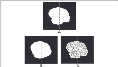
Fig. 4The effect of decreasing the true negatives (background) on the ranking. Each of the segmentations inAandBis compared with the same ground truth. All metrics assess that the segmentation inAis more similar to the ground truth than inB. InA´, the segmentation and ground truth are the same as inA, but after reducing the true negatives by selecting a smaller bounding cube. The metricsRI,GCE, andTNRchange their rankings as a result of reducing the true negatives. Note that some of the metrics are similarities and others are distances
Fig. 5The effect of overlap on the correlation between rankings produced by different metrics. The positions and heights of the bars show how metrics correlate withDICEand how this correlation depends on the overlap between the compared segmentations. Four different overlap ranges are considered
false positives and/or false negatives (decreasing overlap) means increasing the probability of divergent correlation. Another observation is the strongly divergent correla-tion between volumetric similarity (VS) andDICE. This divergence is intuitive since theVSonly compares the vol-ume of the segment(s) in the automatic segmentation with the volume in the ground truth, which implicitly assumes that the segments are optimally aligned. Obviously, this assumption only makes sense when the overlap is high. Actually, theVScan have its maximum value (one) even when the overlap is zero. However, the smaller the over-lap, the higher is the probability that two segments that are similar in volume are not aligned, which explains the strong divergence in correlation when the overlap is low.