Open Access
Research article
Data-driven haemodynamic response function extraction using
Fourier-wavelet regularised deconvolution
Alle Meije Wink*
1, Hans Hoogduin
2and Jos BTM Roerdink
2,3Address: 1Robert Steiner MR Unit, Imaging Sciences Department Imperial College, and MRC Clinical Sciences Centre, Hammersmith Hospital,
London, UK, 2Institute for Behavioral and Cognitive Neurosciences and BCN Neuroimaging Center, Groningen, The Netherlands and 3Institute
for Mathematics and Computing Science, University of Groningen, The Netherlands
Email: Alle Meije Wink* - [email protected]; Hans Hoogduin - [email protected]; Jos BTM Roerdink - [email protected]
* Corresponding author
Abstract
Background: We present a simple, data-driven method to extract haemodynamic response functions (HRF) from functional magnetic resonance imaging (fMRI) time series, based on the Fourier-wavelet regularised deconvolution (ForWaRD) technique. HRF data are required for many fMRI applications, such as defining region-specific HRFs, effciently representing a general HRF, or comparing subject-specific HRFs.
Results: ForWaRD is applied to fMRI time signals, after removing low-frequency trends by a wavelet-based method, and the output of ForWaRD is a time series of volumes, containing the HRF in each voxel. Compared to more complex methods, this extraction algorithm requires few assumptions (separability of signal and noise in the frequency and wavelet domains and the general linear model) and it is fast (HRF extraction from a single fMRI data set takes about the same time as spatial resampling). The extraction method is tested on simulated event-related activation signals, contaminated with noise from a time series of real MRI images. An application for HRF data is demonstrated in a simple event-related experiment: data are extracted from a region with significant effects of interest in a first time series. A continuous-time HRF is obtained by fitting a nonlinear function to the discrete HRF coeffcients, and is then used to analyse a later time series.
Conclusion: With the parameters used in this paper, the extraction method presented here is very robust to changes in signal properties. Comparison of analyses with fitted HRFs and with a canonical HRF shows that a subject-specific, regional HRF significantly improves detection power. Sensitivity and specificity increase not only in the region from which the HRFs are extracted, but also in other regions of interest.
1 Background
In functional magnetic resonance imaging (fMRI), local brain activation temporally changes blood oxygenation, which induces a blood oxygenation level dependent (BOLD) contrast in MR images [1]. Given a model of the
BOLD response to a stimulus pattern, statistics can be used to quantify the match between the predicted and measured signals in a voxel, and significant activation is assessed via hypothesis testing. Statistical parametric map-ping (SPM) estimates parameters of the noise distribution
Published: 10 April 2008
BMC Medical Imaging 2008, 8:7 doi:10.1186/1471-2342-8-7
Received: 17 October 2007 Accepted: 10 April 2008
This article is available from: http://www.biomedcentral.com/1471-2342/8/7
© 2008 Wink et al; licensee BioMed Central Ltd.
in every voxel to determine a threshold for the computed statistic [2]. It uses the general linear model (GLM): the response to a stimulus pattern is modelled as the output of a linear, time invariant (LTI) system [3]. The response to one type of stimulus is modelled by convolving its tem-poral distribution with the response function of that type of stimulus. The total response is the sum of responses to all individual stimulus types. The stimulus pattern is known from the experimental setup. However, the haemodynamic response function (HRF), i.e., the tempo-ral BOLD impulse response, is unknown. Essentially, it is a smooth curve that starts to rise two seconds after the stimulus, peaks after six seconds, and returns to baseline within 30 seconds.
The resolution of discrete fMRI time samples yields a coarse description of the HRF, which is a problem for designs with short and/or randomised stimuli. In slice-wise MRI acquisition, there is no optimal sampling for all slices, and slight differences in temporal onset between voxels in different slices must be accurately modelled to obtain good sensitivity. This requires a continuous-time HRF model. It is sometimes preferable to use a common HRF for many experiments and many regions. In many cases though, a common HRF cannot be assumed [4,5]. Two ways to solve this problem are (i) including a HRF model with more basis functions [5], and (ii) estimating the shape of the HRF in the statistical analysis [4,6]. A drawback of the first and simple approach is that it covers only limited variation in the HRF shape, while more advanced approaches suffer from high complexity and long computation times. For previous work on the varia-bility of the BOLD response between brain areas and even across repeated measurements of the same subject, see Neumann et al. [7].
Extracting a HRF from fMRI data requires assumptions about its shape, and is computationally expensive. A sim-ple method described in the literature is selective averag-ing with a long interstimulus interval (ISI), assumaverag-ing non-overlapping responses [8,9]. Trials with overlapping responses are also averaged, ignoring the fact that the overlaps introduce errors [3,10,11]. Other studies use a functional description of the HRF, whose parameters are determined by curve fitting (examples in [12-14]), one of which [12] uses frequency-domain deconvolution. Another technique based on the GLM expands the HRF into a set of basis functions [15,16].
Ciuciu et al. [4] use a Bayesian method to extract the HRF. The method can simultaneously extract multiple HRFs from multiple experiments. Woolrich et al. [6] use a fully Bayesian approach to fMRI modelling, including the HRF. Both these approaches use certain prior assumptions for the shape of the HRF: in the first case, causality,
smooth-ness, and starting and ending at baseline level, and Gaus-sian temporal autocorrelations; in the second case, a set of predefined prior HRF shapes, and many priors for model-ling the noise distribution and autocorrelation.
The HRF extraction method described here is data-driven
instead of model-driven. It is based on Fourier-wavelet regularised deconvolution, ForWaRD for short, developed originally for denoising and deblurring of images [17].
ForWaRD combines frequency-domain deconvolution for identifying overlapping signals, frequency-domain regu-larisation for suppressing noise, and wavelet-domain reg-ularisation for separating signal and noise. It is related to recent wavelet-based deconvolution techniques [18-20], with the advantage that the roles of signal (for fMRI: sparse, high frequency) and response (for fMRI: smooth, low frequency) can be interchanged: unlike other wavelet-and vaguelette-based deconvolution methods, ForWaRD
does the first step entirely in the frequency domain.
The method described in this paper uses an fMRI data set and the stimulus time pattern, and produces a time series of image volumes, which contains the HRF in each voxel. Compared to the simple extraction methods above, this method has the advantage of taking overlapping responses into account. On the other hand, it is much simpler than the Bayesian ones described above, in that it does not rely on shape assumptions/priors of the HRF: the extracted time points are determined only by the fMRI sig-nal and the stimuli: the method is data-driven. This important property means that the extracted HRF is not biased by any a priori model. The only requirements for
ForWaRD are (i) LTI responses and (ii) separability of sig-nal and noise in the frequency/wavelet domain. Studies of the linearity of the BOLD response indicate that (i) is a reasonable assumption, and given the smoothness of the HRF and the availability of smooth wavelet basis func-tions, (ii) is satisfied as well. Another important advantage is the fact that wavelet-based signal processing methods are much better in preserving the 1/f-type temporal auto-correlations that are found in fMRI time signals than time-domain methods [21]. Models that do not preserve this structure yield biased results, leading to an increase in false positives [21,22]. Finally, our method is fast: HRF extraction from a single fMRI data set takes about the same time as spatial resampling.
with some neural response function (NRF), the exact form of this coupling is still unknown and remains an area of active research. In our method, we describe the haemody-namic response as a convolution of the stimulus (not the LFP) with an impulse response function, i.e., the HRF. Given the stimulus pattern our method can recover the HRF, but we do not claim to be able to extract the NRF via deconvolution.
The output time series can be used to determine subject-specific, group-subject-specific, and region-specific HRFs, e.g., by averaging time signals in the corresponding regions. We demonstrate this in an fMRI experiment using two acqui-sitions, where the HRF extracted from the first fMRI time series is used to predict responses in a second experiment. A functional description for the HRF is found by fitting a combination of two gamma density functions with varia-ble parameters for height, dilation, peak location and lag. We show that contrast and localisation improve by using the extracted HRF instead of the canonical HRF from the SPM2 program (a sum of two gamma density functions (GDFs) with fixed parameters).
The remainder of this paper is organised as follows. Sec-tion 2.2 reviews the ForWaRD method for regularised deconvolution. Sect. 2.2.4 describes how ForWaRD is used for HRF extraction, and it describes how the method was tested on simulated noisy time series and demon-strates a possible application using event-related fMRI data. Sect. 4 contains some general conclusions.
2 Methods
This section briefly reviews the standard General Linear Model (GLM) in fMRI, and describes the ForWaRD
method [17] for extracting the HRF.
2.1 The General Linear Model
Statistical parametric mapping (SPM) is a common analy-sis method for fMRI. It (a) computes a statistic for every voxel using the GLM, (b) chooses a threshold based on the parameters of the noise and multiple testing correction; (c) thresholds the statistic map.
The GLM describes the response in an fMRI experiment as a weighted sum of explanatory signals. An explanatory sig-nal is the response of one stimulus type. Let the matrix
Y[T×N] denote the fMRI data set, whose elements yij have
time index i = 1, ..., T and position index j = 1, ..., N . In the GLM,
Y = Xβ+ e. (1)
X[T×M] is the design matrix, whose columns are the
explan-atory signals, and are multiplied by the weights in matrix
β[M×N]. Matrix e[T×N] is the residual signal for each yij. A
least-squares estimate b for β is given by (XTX)-1XTY .
Assuming a Gaussian temporal distribution of the residu-als (this follows from the GLM if the temporal noise in Y
is Gaussian), standard hypothesis testing can be used to assess the significance of the elements of b.
2.2 Deconvolution, ForWaRD, and HRF extraction
In the GLM, a single response g to a pattern f of stimuli of the same type, is a convolution of f with the impulse response h, plus an additive term representing noise and other confounding effects.
2.2.1 Deconvolution
Discrete circular convolution, denoted by '*', corresponds to multiplication in the frequency domain:
g(n) = (h * f)(n) + e(n) G(k) = H(k)F(k) + E(k), (2)
capital letters denoting Fourier transforms of the corre-sponding lower-case signals. In the absence of noise, and given g and f, it is possible to compute an estimate of h
through deconvolution. In the frequency domain, the Fourier transform of is obtained by pointwise divi-sion:
Deconvolution of a noisy signal is an ill-posed problem. A unique solution may not exist, be meaningless, or at best unstable: if noise is amplified at frequencies k where
F(k) is close to zero, parts of the unmodelled signal e may appear in the extracted response (see Fig. 2i). An ill-posed problem can be regularised by adding extra information (or constraints) to the problem, so that its solution approximates the noise-free case [24]. Examples of such constraints are: minimising the norm between the solu-tion and the data (minimum-norm), and making the solution more stable (smooth around optimum). For-WaRD uses regularisation methods in the frequency and wavelet domains (see Fig. 1) to overcome this problem.
2.2.2 Fourier shrinkage
Frequency-domain shrinkage attenuates the noise after the pointwise division, by multiplying each frequency coeffcient (k) by a factor λ(k). Two popular methods are Wiener shrinkage and Tikhonov shrinkage [17]:
h
H h
H k H k E k
F k F k k N
( ) ( ) ( )
( ), | ( ) |
, ,
... .
= + >
Here is the variance of the noise e(n) in (2). The remarks at the end of this subsection explain how to esti-mate and determine optimal regularisation parame-ters αand τ. An estimate of the spectrum |H(k)|2 of the unknown response function needed for Wiener shrinkage is obtained by the iterative algorithm of Hillery and Chin [[25], Sect. 4]. The estimated response function is the inverse Fourier transform of (see Fig. 2ii).
2.2.3 Wavelet shrinkage
Shrinkage in the wavelet domain is done using wavelet-domain Wiener shrinkage (WDWS), which reduces the noise and preserves details in the signal [17,26]. The dis-crete wavelet transform describes a sampled signal c0 of
length N as a sum of localised basis functions. A discrete wavelet transform with J levels of decomposition recursively splits the signal into an approximation part cJ
and detail signals d1, d2, ..., dJ, which are weighted sums of shifted and dilated versions of a scaling function φand an associated wavelet ψ, respectively. The fast wavelet trans-form [27], which pertrans-forms downsampling at each level, is not shift-invariant. ForWaRD uses a shift-invariant dis-crete wavelet transform (SI-DWT), which uses a polyphase decomposition (subsampling for all shifts) [28]. Recon-struction is possible via the inverse transform, denoted by SI-IDWT.
WDWS is performed via two wavelet transforms (for details, see [[17], section IV.C]). First, a wavelet transform
of is computed using (φ1, ψ1). A pilot estimate is
obtained via scale-dependent thresholding of the detail coeffcients , resulting in thresholded detail coef-fcients , n =1,...,N. Another wavelet transform of
with wavelet basis (φ2, ψ2) yields detail coeffcients . These are shrunk by wavelet-Wiener filtering coeffcients:
Here is the noise variance at level j. Finally, the
For-WaRD estimate is the SI-IDWT of the shrunk
coef-fcients using wavelet basis (φ2, ψ2), see Fig. 2iii.
Remarks:
• The variance σe is estimated based on the median
abso-lute detail (MAD) coeffcient of a one-level wavelet trans-form [[29], §5.4] of the the noise e(n).
• In the frequency-domain shrinkage step, the parameters
τ(Tikhonov) and α (Wiener) can be tuned to minimise the mean squared error (MSE) between the estimate and the exact response function h. The exact MSE cannot
H k H k k
k F k F k F k F k λ λ λ τ ( ) ( ) ( ) ( ) | ( )| | ( )| ( ) | ( )| | ( = = + 2 2 2 Tikhonov ))| /| ( )| ( ) 2+ 2 2
⎧ ⎨ ⎪ ⎪⎪ ⎩ ⎪ ⎪
⎪ α σ εN H k
Wiener
(4)
σε2
σε2
hλ
Hλ
J∈N
hλ
{ ( )}d n1j 1J
{ ( )}d n1j 1J
hλ
{ ( )}d n2j 1J
ˆ ( ) ( ) | ( )| | ( )|
, ,
d n d n d
j n
dj n j
j j
j n j n
2 2 1
2
1 2 2
= =
+
κ κ
σ (5)
σ2j
hλ κ,
(c2J,{ }d2j jJ=1)
hλ κ,
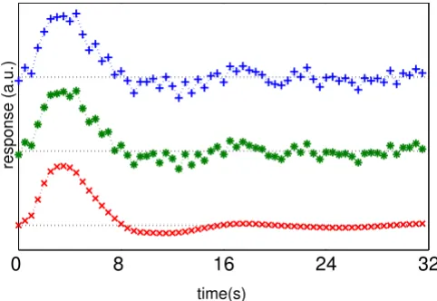
Stages of ForWaRD Figure 2
Stages of ForWaRD. HRF coeffcients after: frequency domain inversion (+); frequency domain shrinkage (*); wavelet domain Wiener shrinkage (×).
ForWaRD HRF extraction scheme Figure 1
be computed, but it can be approximated very accurately, see [[17], section VII].
• A complete Matlab implementation of the original For-WaRD algorithm, on which our method is based, is avail-able 1
2.2.4 Using ForWaRD for HRF extraction
The ForWaRD-based HRF extraction scheme (see Algo-rithm 1) works as follows: The BOLD response to a stim-ulus pattern f is relative to the baseline. Low-frequency trends in the baseline may contaminate the extracted HRF. Trends are removed beforehand by a standard wavelet-based technique [30]: transform each time signal (with length N) to the wavelet domain, using a fast wavelet transform (FWT) of log2(N) - 3 levels; remove the detail coeffcients, and subtract the low-scale signal from the time series. The influence of the detrending on the For-WaRD estimates is minimal, because the low-pass trends are in a much lower frequency band than the HRF. Processing takes place on a voxel-by-voxel basis, so images can be partitioned to reduce the computation load. The output is a time series of volumes which, inside activated brain areas, contain the HRF. Implementation has been performed in Matlab (The Mathworks, USA).
Algorithm 1 ForWaRD-based HRF extraction scheme.
1: for all Voxels do
2: load the discrete time series g and stimulus pattern f;
3: compute and subtract the time series mean;
4: remove low-frequency trends;
5: apply ForWaRD to the mean-corrected and detrended signal g and stimulus pattern f to obtain the estimate of the HRF coeffcients.
6: end for
2.3 Tests on simulated fMRI time signals
The routine presented in Sect. 2.2.4 was tested on signals with varying properties (SNR, temporal resolution, low-frequency trends) with different settings of the routine itself (decomposition level, wavelet filters, etc.). Figures 3a–d shows the test setup: (a) convolve a stimulus pattern with a known HRF to obtain the activation signal; (b) add noise and a low-pass trend to it to obtain the total response; (c) recover the HRF from this total response, and (d) reconstruct the activation signal by convolving the stimulus pattern with the recovered HRF. The MSE
between the activation signal and the reconstructed ver-sion was used to measure the reconstruction accuracy.
2.3.1 Simulation of fMRI time signals
128 EPI scans of a subject at rest were acquired on a 3T Intera system (Philips Medical Systems, The Netherlands), with repetition time (TR) 3 s, image size 64 × 64 × 46 vox-els of 3.5 × 3.5 × 3.5 mm3. A total of 512 noise time
sig-nals were collected from a region of 8 × 8 × 8 voxels (see Fig. 4). A randomised stimulus pattern f(n), n = 1, ..., N
was obtained by thresholding a vector of random values. The stimulus f(n) n = 1, ..., N was convolved with an impulse response function h(n), in this case the canonical haemodynamic response function HRFspm, to describe the activation signal s(n). HRFspm(t) (see Fig. 3f) is the
differ-ence of two gamma density functions (GDF),
where the GDF γm, l(t) has the form:
Four types of low-frequency trends: flat, linear, sinusoidal and quadratic (see Fig. 5a) were added to the signal. The SNR of the time signals was set by choosing the standard deviations σs of the signal and σe of the noise, as well as the scalar mn such that
Trends with standard deviation σt > 0 were scaled by mt so that mtσt = mnσe. The time signal in each voxel was the sum {EPI noise} + {activation} + {trend} (Fig. 3b). Tests included time signals with varying (a) input SNR, (b) low-frequency trends, (c) repetition time (TR), and (d) response onset.
2.3.2 Reconstruction of activation signals
The HRF was extracted from each time signal by the For-WaRD-based routine, and the mean HRF was used to reconstruct the activation signal by convolving it with the stimulus pattern. The following settings of the ForWaRD -routine were varied: (a) type of frequency shrinkage, (b) levels of the wavelet transform, (c) wavelet-domain threshold level, and (d) the wavelet basis. The default val-ues were: SNR 0 dB, no trend, TR 2 s, onset delay 0 s, Tikhonov shrinkage, τ0.1, decomposition level 3, θ3, φ1 Daubechies-4, φ2 Daubechies-3 [31].
hλ κ,
HRFspm( )t =γ6 1,( )t − γ16 1,( ),t
1
6 (6)
γm l t m t
lmt m e lt
m m t e t
,( ) ( ) , ( ) . = − − = ∞ − −
∫
1 1 0Γ Γ d (7)
SNR=10log10 σ .
σs
Test set-up Figure 3
2.4 Event-Related fMRI experiments
An application of the HRF extraction method is demon-strated in an event-related fMRI experiment. HRF coef-fcients were extracted from the fMRI data set, and HRFs were computed by fitting a model function to HRF coef-fcients (both whole-brain and region-of-interest). These HRFs were then used in a subsequent GLM-based analysis.
2.4.1 Fixed-ISI experiment
The subject in the MRI scanner had to make a fist on the appearance of a visual stimulus, and relax after 1 s. Cues were given on a white screen placed inside the scanner: a red disc was a cue to make a fist, a white disc meant that the subject had to rest. The experiment consisted of 156 scans, acquired as described in Sect. 3.1. Cues were given every 24 s (8 scans × 3 s, no jittering), starting at scan 2. Increased task-related activity was expected in the motor
cortex, the premotor cortex, the supplementary motor area and the cerebellum.
The EPI data were denoised with a wavelet-based tech-nique [32], using SUREShrink in the wavelet domain [29]. Realignment, normalisation, and statistical analysis were done with SPM2 [2]. Slice timing correction was not applied. The design matrix X contained a set of 6 Fourier basis functions (3 sines, 3 cosines) modulated by a Han-ning window, in the time interval of 8 scans after each stimulus, and a constant signal modelling the time series mean. The Fourier basis was used to model a large class of signals using only few assumptions.
The variance ratio [33] was computed in each voxel, and an F-test was used to determine significance. False discov-ery rate (FDR) control [34] with q = 0.05 was used to cor-rect for multiple hypothesis testing.
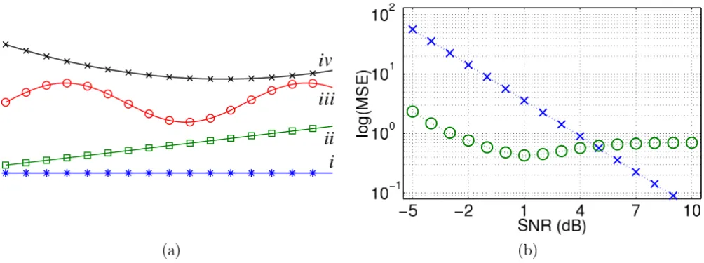
(a) Low-frequency trends: (i) flat, (ii) linear, (iii) sinusoidal, (iv) quadratic Figure 5
(a) Low-frequency trends: (i) flat, (ii) linear, (iii) sinusoidal, (iv) quadratic. (b) log10(MSE) of noisy (×) and reconstructed (o) sig-nals given the input SNR.
Area sampled from EPI data: (a) transverse, (b) sagittal, (c) coronal Figure 4
2.4.2 Random-ISI experiment
A second experiment used a random stimulus sequence, created by thresholding a sequence of random values (39 stimuli, ISI mean: 6.05 scans, σ: 4.31 scans, no jittering). The number of scans was 256, scanning parameters and preprocessing were as in Sect. 3.1.
Due to overlapping responses, the windowed Fourier basis set could not be used. It was replaced by the canon-ical HRF from the SPM2 program and its time and dila-tion derivatives. An F-test of the variance ratio with FDR q
= 0.05 was used to assess significance.
2.4.3 Extracting and modelling HRFs from the time series
A stricter FDR-corrected threshold (q = 0.0001) was applied to the variance ratio maps, sampling the HRF in a smaller number of voxels.
A continuous HRF was obtained by fitting a generalised version of HRFspm (6) to the coeffcients returned by
For-WaRD and selective averaging. We use HRFgam to denote the difference of two GDFs with 8 parameters, i.e.,
H(eight), D(ilation), P(eak location) and L(ag) of both GDFs:
Levenberg-Marquardt's nonlinear curve-fitting algorithm was used to determine these parameters and 95% predic-tion intervals for the fitted funcpredic-tions.
2.4.4 Using fitted HRFs to model responses
HRFs measured from an fMRI data set cannot be used to test for activation in that same data set: a model must be specified a priori, so that inferences are not made from models that are determined by the data itself. We tested for activation in the random-ISI experiment with the HRFs fitted to the coeffcients extracted from the fixed-ISI data, and vice versa. The GLM was estimated using the stimulus times and the fitted HRFs, and their correlation the fMRI time signals was computed. Significance was determined via a one-sample t-test, and FDR control with q = 0.05 was used to correct for multiple hypothesis testing.
3 Results
3.1 Simulated fMRI time signals
The properties of the signal and parameters of the extrac-tion routine that noticeably influenced the original activa-tion signal s(n) and its reconstruction r(n), are listed below.
3.1.1 Output MSE as a function of input SNR
Figure 5b shows the MSE for various input SNR values. For input SNRs up to 9 dB the MSE decreases; it increases above 9 dB.
3.1.2 Choice of shrinkage type and τ parameter
Wiener shrinkage uses an iterative algorithm [25] to esti-mate |H|2 (see (4)), the number of iterations was limited
to 10. Figure 6 shows the MSE for both types of frequency domain shrinkage, varying SNR and regularisation param-eter τ. For low SNR and heavy regularisation (τ ≥ 1), Tikhonov regularisation outperforms Wiener shrinkage. For higher SNRs or mild regularisation, Wiener shrinkage performs better. The best value for τ depends on the shrinkage type, the SNR and the TR. For short TR, mild regularisation (τ ≤ 0.1) is preferable. A long TR requires heavy regularisation.
3.1.3 Different response delays
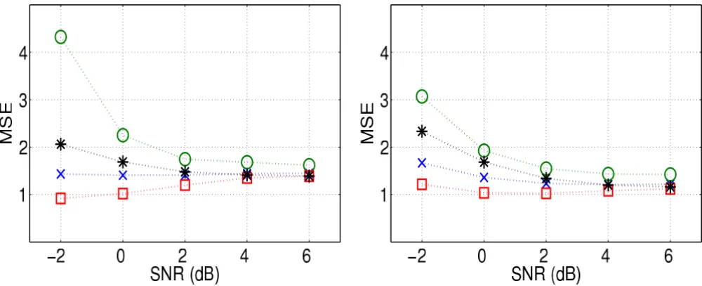
Figure 7 shows that HRFs with different onset delays can equally well be extracted with ForWaRD. The MSE hardly changes with different delays, indicating that the shape of the response is preserved. The increased MSE for negative shifts is caused by the fact that the HRF was only sampled post-stimulus.
3.1.4 Different wavelet filters
We tested 15 different wavelet filters for (φ1, ψ1), as well as for (φ2, ψ2): Daubechies wavelets 1 ... 5 (the filter number indicates the number of vanishing moments), Daubechies' symmetric wavelets 2 ... 6 [35] (filter 1 corre-sponds to the Daubechies-1 filter), and Coiflets 1 ... 5 [35]. Different filters did not yield large differences in per-formance.
3.1.5 Decomposition level and noise threshold
Figure 8 shows the MSE for different SNRs, different θand different decomposition levels. We find that two-level decompositions produce the smallest errors for the lower SNRs, and three-level decompositions perform best for the higher. Four-level and five-level decompositions yield higher errors. A higher θoften yields a lower MSE.
3.1.6 Different low-frequency trends
Tests with low-frequency trends (see Fig. 5a) show that the type of frequency domain shrinkage changes the result. (see Fig. 9). The MSE is higher with Tikhonov than with Wiener shrinkage, especially for lower SNRs. Trends are not removed perfectly with either shrinkage type, but the extra information about f and the power spectral density of h in Wiener shrinkage make it less sensitive to trend residuals.
HRFgam( )t =H1γP D1, 1(t−L1)−H2γP D2, 2(t−L2).
3.1.7 Summary
Even though the default parameters (see Sect. 2.3.2) make the algorithm robust for a wide range of signals (different SNR, sampling frequency, etc.), the method is also robust changing its parameters, such as the wavelet filters and decomposition level. The MSE of the reconstructed signal was lower than the input MSE in most of the tested situa-tions.
The robustness to onset delay makes ForWaRD an attrac-tive alternaattrac-tive to other delay correction methods such as including a temporal derivative of the standard HRF in the model [16]: these only correct for small synchronisation
errors, and are not usable when the HRF is not well mod-elled by the standard function.
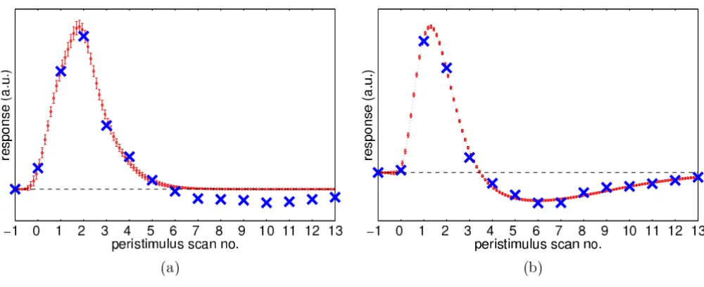
3.2 Event-related fMRI: fixed-ISI
Activation maps are shown in Fig. 10a as 'glass brain' max-imum intensity projections (MIP) in two orthogonal directions. Low statistic values are shown in grey, high val-ues in black. The highest value is indicated with a '<' sign. Activation was found in the expected areas, predomi-nantly in the motor cortex. A whole-volume HRF was extracted from the post-stimulus volumes using selective averaging [9], by taking the mean response of each vol-ume, weighted by the map of significant statistic values. A
Output MSEs of Tikhonov (left) and Wiener (right) shrinkage with a TR of 0.5 s (top) and 3 s (bottom), for different input SNRs and a varying regularisation parameter τ× τ= 0.01, o τ= 0.1, : τ= 1, *: τ= 10
Figure 6
region-specific HRF in the 7 × 7 × 7-voxel neighbourhood of a selected voxel (see the '<' in Fig. 10a) was computed by using only the time signals from that region. Figure 11a–b shows the extracted HRFs.
The ForWaRD algorithm used 128 scans of the experi-ment, starting with scan 2 (first stimulus). Whole-volume
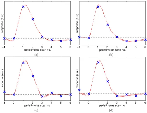
HRF and region-specific HRF time points were computed using the post-stimulus time series (see Fig. 11c–d). The HRFs extracted by ForWaRD are similar to the results from selective averaging, except that the baseline of the For-WaRD-extracted HRF decreases. This is because the HRF does not return to baseline within the sampled interval (24 s), so in the GLM the response decreases at the end of
Output MSE for varying response onset delays, for Tikhonov (left) and Wiener (right) shrinkage, SNR = -2 dB (×), 0 dB (o), 2 dB ( ), 4 dB (*), and 6 dB (+)
Figure 7
Output MSE for varying response onset delays, for Tikhonov (left) and Wiener (right) shrinkage, SNR = -2 dB (×), 0 dB (o), 2 dB ( ), 4 dB (*), and 6 dB (+).
Output MSE for different SNRs, with various levels of decomposition and threshold levels Figure 8
every stimulus. In some cases (see Fig. 11c–d) this was fixed manually by setting the baseline to the last HRF coef-fcient.
3.3 Event-related fMRI: random-ISI
The contrast of the random-ISI experiment was generally weaker than in the fixed-ISI experiment, but localisation was better, see Fig. 10b.
A post-stimulus time series was made with ForWaRD, using all 256 scans of the experiment. Selective averaging could not be used because of overlapping responses. With a random ISI, a much longer post-stimulus interval can be sampled [11]. The post-stimulus volumes produced by the extraction routine were used to create a whole-volume
HRF and a region-specific HRF in the same way as in the fixed-ISI case.
Figure 12 shows the extracted HRF coeffcients and the fit-ted HRFs. A comparison between Fig. 11c–d and Figure 12 shows that the ForWaRD-extracted HRF coeffcients from the random-ISI design agree better with the model func-tion than those from the fixed-ISI design, especially in the region-specific case. A possible explanation is that the fixed-ISI stimulus signal does not contain enough fre-quency information to do the Fourier inversion, resulting in a lower-quality estimate. In contrast, selective averaging does not work with overlapping responses and random ISIs.
Maps of the variance ratio using the F-test with FDR q = 0.05 Figure 10
Maps of the variance ratio using the F-test with FDR q = 0.05. The highest value is indicated with a '<' sign. (a) Fixed-ISI exper-iment, range 3.86–20.63 and (b) random-ISI experexper-iment, range 5.43–41.63 (b). The indicated areas are: l.motor cortex (1),
sup-Output MSE for different SNRs and low-pass trends in the data Figure 9
3.4 Activation detected with fitted HRFs
Figure 13 shows the activation detected in the fixed-ISI dataset with the HRFs extracted by ForWaRD from the ran-dom-ISI dataset. There is good correspondence between the maps of the whole-volume (a) and region-specific (b) HRFs, respectively, and the detected activations match the expected pattern (see Fig. 10). Figure 14 shows the activa-tion detected in the random-ISI dataset with the HRFs from the fixed-ISI dataset, using both selective averaging (a-b) and ForWaRD (c-d), which are in very good agree-ment. Where selective averaging is possible, ForWaRD
yields results very similar to those produced by selective averaging. The statistical maps for ForWaRD between the fixed-ISI and random-ISI time series are in good corre-spondence.
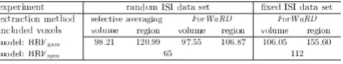
An analysis was also performed performed with the gen-eral HRFspm. The activation maps in Fig. 13 are in very good correspondence with Fig. 15a, indicating that both HRFspm and HRFgam model the data well. The values for the variance ratio in Fig. 16 for the fixed-ISI experiment show that all models explain the data well, and HRFgam with the regional HRF yields the best fit to the data.
Figures 14 and 15b show that HRFspm yields a poor fit to the data; this is also shown in Fig. 16. The higher variance ratios for HRFgam indicate that a larger portion of the measured variance is explained by the model, and that the residual of the GLM (1) is small. The fitted region-specific HRFs generally perform better than whole-volume HRFs, and the maps of detected activation indicate that the fitted HRFs do not only detect activation in the region from
HRFs extracted from the fixed-ISI data by selective averaging (top row) and ForWaRD (bottom row) Figure 11
which they were extracted, but that they are general enough to also detect activation in other areas, corre-sponding to the predicted activated regions (see the blue ellipses in Fig. 10).
4 Conclusion
We have developed a technique to extract HRF coeffcients from fMRI time series based on the ForWaRD deconvolu-tion technique. Frequency-domain deconvoludeconvolu-tion allows extraction of the HRF even when the responses to subse-quent stimuli overlap, and the sensitivity to noise of fre-quency-domain deconvolution is compensated by Wiener or Tikhonov shrinkage in the frequency domain, followed by wavelet-domain Wiener shrinkage. Before applying
ForWaRD, low-frequency trends are removed from the time signal with a standard wavelet-based method. Tests
of the extraction routine using simulated activation, sev-eral types of trend and noise from a real fMRI time series, demonstrate its robustness. Results show that the method is robust to trends in the data, and the performance does not differ much between the noise levels we tested. The output of our algorithm is a post-stimulus time series, rep-resenting the HRF coeffcients in every voxel. At present, the extraction method is capable of recovering one HRF from one time series. The algorithm used in this paper is entirely data-driven: it does not use a priori models of the data. Other advantages of this algorithm are its simplicity,
i.e., the algorithm works independently of other pre- and postprocessing steps; and its speed and low computa-tional complexity.
Activation in the fixed-ISI data set, using the F-test with FDR q = 0.05 Figure 13
Activation in the fixed-ISI data set, using the F-test with FDR q = 0.05. The highest value is indicated with a '<' sign. HRFs extracted from the random-ISI data set by ForWaRD and modelled with HRFgam. (a) whole-volume HRF, range 3.08–10.62. (b) region-specific HRF, range 2.99–12.72.
HRFs extracted from the random-ISI experiment by ForWaRD: whole-volume (a) and region-specific (b) Figure 12
The default settings of the method used in the tests as well as in the fMRI experiments (see Sect. 2.3.2) lead to a good and robust performance of the extraction algorithm.
We have demonstrated the use of ForWaRD-extracted HRFs in combination with continuous HRF functions to predict event-related fMRI responses. Given the output of the extraction routine, continuous functions (in this case gamma densities) are fitted to the average HRF coeffcients in a region of a (statistical or anatomical) map.
Results from the experiments with extracted and fitted HRFs indicate that subject-specific and region-specific HRFs lead to stronger contrasts and better localisation than a standard HRF. The results with the random-ISI data suggest that it is possible to use ForWaRD in combination with relatively complex prior experiments to extract HRFs, and that it is beneficial to use these HRFs instead of stand-ard functions for detection and modelling of subse-quently acquired data. The advantage of using a single, tailored HRF over a model that spans several basis func-tions, is that the statistical analysis is more specific and
Activation maps of the fixed-ISI data set (a, range 3.10–10.80), and the random-ISI data set (b, range 3.32–8.61), using HRFspm
Figure 15
Activation maps of the fixed-ISI data set (a, range 3.10–10.80), and the random-ISI data set (b, range 3.32–8.61), using HRFspm. The highest value is indicated with a '<' sign.
Activation maps of the random-ISI data set, using the F-test with FDR q = 0.05 Figure 14
more powerful, resulting in a stronger contrast and better localisation.
A possible extension of the method is the extraction of multiple HRFs from one or multiple experiments. Decon-volution in the frequency domain of multiple waveforms has already been done in ERP research [36]. The For-WaRD-based method may be extended in a similar way.
Competing interests
The author(s) declare that they have no competing inter-ests.
Authors' contributions
AMW wrote the software, did the analyses and wrote most of the paper. JBTMR designed critical parts of the method and coauthored the paper. HH led the image acquisition.
Note
Figure 16 Maximum variance ratio values found in the tests.
1http://www.dsp.rice.edu/software
Acknowledgements
This research is part of the project "Wavelets and their applications", funded by the Dutch National Science Foundation (NWO), project no. 613.006.570.
References
1. Ogawa S, Lee TM, Kay AR, Tank DW: Brain Magnetic Resonance Imaging with Contrast Dependent on Blood Oxygenation. Proceedings of the National Academy of Sciences 1990, 87:9868-9872. 2. Friston KJ, Holmes AP, Worsley KJ, Poline JP, Frith CD, Frackowiak
RSJ: Statistical Parametric Maps in Functional Imaging: A General Linear Approach. Human Brain Mapping 1995, 2:189-210 [http://www.fil.ion.ucl.ac.uk/spm].
3. Boynton GM, Engel SA, Glover GH, Heeger DJ: Linear Systems Analysis of Functional Magnetic Resonance Imaging in Human V1. The Journal of Neuroscience 1996, 16(13):4207-4221. 4. Ciuciu P, Poline JB, Marrelec G, Idier J, Pallier C, Benali H:
Unsuper-vised robust non-parametric estimation of the hemody-namic response function for any fMRI experiment. IEEE Transactions on Medical Imaging 2003, 22(10):1224-1234.
5. Handwerker DA, Ollinger JM, D'Esposito M: Variation of BOLD hemodynamic responses across subjects and brain regions and their effects on statistical analyses. NeuroImage 2004,
21(4):1639-1651.
6. Woolrich MW, Jenkinson M, Brady JM, Smith SM: Fully Bayesian spatio-temporal modeling of FMRI data. IEEE Transactions on Medical Imaging 2004, 23(2):213-231.
7. Neumann J, Lohmann G, Zysset S, von Cramon DY: Within-subject variability of BOLD response dynamics. Neuroimage 2003,
19(3):784-796.
8. Bandettini PA, Cox RW: Event-Related fMRI Contrast When Using Constant Interstimulus Interval: Theory and Experi-ment. Magnetic Resonance in Medicine 2000, 43:540-548.
9. Buckner RL, Bandettini PA, Craven KMO, Savoy RL, Petersen SE, Rai-chle ME, Rosen BR: Detection of cortical activation during averaged single trials of a cognitive task using functional magnetic resonance imaging. Proceedings of the National Academy of Sciences 1996, 93:14878-14883.
10. Zarahn E, Aguirre G, D'Esposito M: A Trial-Based Experimental Design for fMRI. NeuroImage 1997, 6:122-138.
11. Burock MA, Buckner RL, Woldorff MG, Rosen BR, Dale AM: Rand-omized Event-Related Experimental Designs Allow for Extremely Rapid Presentation Rates Using Functional MRI. NeuroReport 1998, 9:3735-3739.
12. Glover GH: Deconvolution of Impulse Response in Event-Related BOLD fMRI. NeuroImage 1999, 9:416-429.
13. Miezin FM, Macotta L, Ollinger JM, Petersen SE, Buckner RL: Char-acterizing the Hemodynamic Response: Effects of Presenta-tion Rate, Sampling Procedure and the Possibility of Ordering Brain Activity Based On relative timing. NeuroIm-age 2000, 11:735-759.
14. Hinrichs H, Scholz M, Tempelmann C, Woldorff MG, Dale AM, Heinze HJ: Deconvolution of Event-Related fMRI Responses in Fast-Rate Experimental Designs: Tracking Amplitude Varia-tions. Journal of Cognitive Neuroscience 2000, 12(6(suppl 2)):76-89. 15. Josephs O, Turner R, Friston KJ: Event-Related fMRI. Human Brain
Mapping 1997, 5:243-248.
16. Friston KJ, Fletcher P, Josephs O, Holmes A, Rugg MD, Turner R:
Characterizing Differential Responses. NeuroImage 1998,
7:30-40.
17. Neelamani R, Choi H, Baraniuk RG: ForWaRD: Fourier-Wavelet Regularized Deconvolution for Ill-Conditioned Systems. IEEE Transactions on Signal Processing 2004, 52(2):418-433.
18. Johnstone I, Kerkyacharian G, Picard D, Raimondo M: Wavelet deconvolution in a periodic setting. Journal of the Royal Statistical Society 2004, 66(3):547-573.
19. Kalifa J, Mallat S, Rouge B: Deconvolution by thresholding in mir-ror wavelet bases. IEEE Transactions on Image Processing 2003,
12(4):446-457.
20. Sanchez-Avila C: Wavelet domain signal deconvolution with singularity-preserving regularization. Mathematics and Comput-ers in Simulation 2002, 2101:1-12.
21. Bullmore ET, Long C, Suckling J, Fadili J, Calvert G, Zelaya F, Carpen-ter TA, Brammer M: Colored Noise and Computational Infer-ence in Neurophysiological (fMRI) Time Series Analysis: Resampling Methods in Time and Wavelet Domains. Human Brain Mapping 2001, 12:61-78.
22. Zarahn E, Aguirre GK, D'Esposito M: Empirical Analyses of BOLD fMRI Statistics: I. Spatially Unsmoothed Data Col-lected under Null-Hypothesis Conditions. NeuroImage 1997,
5:179-197.
23. Logothetis NK, Pauls J, Augath M, Trinath T, Oeltermann A: Neuro-physiological Investigation of the Basis of the fMRI Signal. Nature 2001, 412:150-157.
24. Kilmer ME, O'Leary DP: Choosing Regularization Parameters in Iterative Methods for Ill-Posed Problems. SIAM Journal on Matrix Analysis and Applications 2000, 22(4):1204-1221.
25. Hillery AD, Chin RT: Iterative Wiener Filters for image resto-ration. IEEE Transactions on Signal Processing 1991, 39:1892-1899. 26. Ghael SP, Sayeed AM, Baraniuk RG: Improved Wavelet
Denois-ing via Empirical Wiener FilterDenois-ing. Proc SPIE: Wavelet Applications in Signal and Image Processing 1997, 3169:389-399.
27. Mallat SG: A Theory for Multiresolution Signal Decomposi-tion: The Wavelet Representation. IEEE Transactions on Pattern Analysis and Machine Intelligence 1989, 11(7):674-693.
28. Holschneider M, Kronland-Martinet R, Morlet J, Tchamitchian P: A real-time algorithm for signal analysis with the help of the wavelet transform. Wavelets, Time-Frequency Methods and Phase Space 1989:286-297.
29. Donoho DL, Johnstone IM: Adapting to Unknown Smoothness by Wavelet Shrinkage. Journal of the American Statistical Association
1995, 90:1200-1224.
30. Meyer FG: Wavelet-based estimation of a semiparametric generalized linear model of fMRI time-series. IEEE Transactions on Medical Imaging 2003, 22(3):315-322.
Maximum variance ratio values found in the tests Figure 16
Publish with BioMed Central and every scientist can read your work free of charge "BioMed Central will be the most significant development for disseminating the results of biomedical researc h in our lifetime."
Sir Paul Nurse, Cancer Research UK
Your research papers will be:
available free of charge to the entire biomedical community
peer reviewed and published immediately upon acceptance
cited in PubMed and archived on PubMed Central
yours — you keep the copyright
Submit your manuscript here:
http://www.biomedcentral.com/info/publishing_adv.asp
BioMedcentral 31. Daubechies I: Orthonormal Bases of Compactly Supported
Wavelets. Communications on Pure and Applied Mathematics 1988,
41:909-996.
32. Wink AM, Roerdink JBTM: Denoising functional MR images: a comparison of wavelet denoising and Gaussian smoothing. IEEE Transactions on Medical Imaging 2004, 23(3):374-387.
33. Josephs O, Henson RNA: Event-related Functional Magnetic Resonance Imaging: Modelling, Inference and Optimization. Philosophical Transactions of the Royal Society 1999, 354:1215-1228. 34. Genovese CR, Lazar NA, Nichols TE: Thresholding of Statistical
Maps in Functional Neuroimaging Using the False Discovery Rate. NeuroImage 2002, 15:772-786 [http://www.sph.umich.edu/ ~nichols/FDR].
35. Daubechies I: Orthonormal Bases of Compactly Supported Wavelets: II. Variations on a Theme. SIAM Journal on Mathemat-ical Analysis 1993, 24(2):499-519.
36. Hansen JC: Separation of Overlapping Waveforms Having Known Temporal Distributions. Journal of Neuroscience Methods
1983, 9:127-139.
Pre-publication history
The pre-publication history for this paper can be accessed here: