Integrative Approaches to Reconstruct Regulatory Networks From Multi-Omics Data: A Review of State-of-the-Art Methods

Integrative approaches to reconstruct regulatory

networks from multi-omics data: A review of

state-of-the-art methods

Nisar Wani, Khalid Raza

F

Abstract—Data generation using high throughput technologies has led to the accumulation of diverse types of molecular data.These data have different types (discrete,real,string etc.) and occur in various formats and sizes. Datasets including gene expression, miRNA expression, protein-DNA binding data (ChIP-Seq/ChIP-ChIP), mutation data(copy number variation, single nucleotide polymorphisms), GO annotations, protein-protein interaction and disease-gene association data are some of the commonly used genomic datasets to study biological processes. Each of them provides a unique, complementary and partly independent view of the genome and hence embed essential information about their regulatory mechanisms. In order to understand the functions of genes, proteins and analyze mechanisms arising out of their inter-actions, information provided by each of these datasets individually may not be sufficient. Therefore integrating these multi-omic data and inferring regulatory interactions from the integrated dataset provides a system level biological insights in predicting gene functions and their phenotypic outcomes. To study genome functionality through interaction networks, different methods have been proposed for collective mining of information from an integrated dataset. We survey here data integration approaches using state-of-the-art techniques such as network integra-tion, Bayesian networks, regularized regression (LASSO) and multiple kernel learning methods.

Index Terms—network inference, data integration, regulatory net-works,transcription factor, gene expression

1

I

NTRODUCTION

L

IVING cells belong to a class of highly studied com-plex systems, whose functioning continues to allure the research community. The cell houses a diverse molecular structure, comprised of a large number of molecular entities viz. genes, proteins, metabolites and mRNA, forming a complex and dynamic molecular machinery. Earlier, experi-mental approaches used to focus on the effect of individual molecular entities or environmental factors to study a par-ticular cell function, without taking into consideration the effect of other important factors. However, these methods are limited by the scale and time of the study, hence making it difficult to obtain a system-wide cellular response of a stimulus e.g., a drug dose, an environmental perturbation or a gene knockdown experiment.

• Nisar Wani ,Govt. Degree College Baramulla,J& K,India.

• Dr. Khalid Raza, Department of Computer Science, jamia Milia Is-lamia,New Delhi India. E-mail: ([email protected]).

For a holistic measurement of cellular responses and identification of functions, novel, high throughput tech-nologies that generate genome-scale data sets open global perspectives of living organisms at the molecular level. Such a collective quantification and characterization of pool of diverse bio-molecules that give rise to structure, function and dynamics of organism is what is commonly nowadays referred to as Omics layers (Gligorijevi´c & Prˇzulj, 2015). For example, a whole set of proteins and their interactions form the proteome , mRNA abundance together with factors responsible for transcription give rise to a transcriptome, genes within the DNA form the genome, metabolites within the cell form metabolome and the diverse phenotypes as phenome. The mechanisms which translate the functional codes within the genome depend on various intermedi-ate omics layers and their inter-relationships (interactome) giving rise to complex phenotypic traits in the phenome (Gligorijevi´c & Prˇzulj, 2015).

High throughput technologies such as , protein mass spectrometry, yeast two-hybrid assays, microarrays and a range of protocols under the banner of next generation sequencing (NGS) viz; RNA-seq, ChIP-seq, DNase-seq and miRNA-seq etc. produce vast amounts of disparate biologi-cal data (Omics), these data sets together with a knowledge-base of experimental literature on biochemical processes are disrupting earlier notion of isolated functionality and linear causality pathways and challenging us with multiple func-tions. For example, a protein produced from the information contained in a genetic sequence may function as a tran-scription factor (TF) binding to regulatory sites on promoter region of a gene or multiple genes, an enzyme responsible for catalyzing a metabolic reaction, a cellular component or as a component of signal transduction pathway, thereby implying networks of interacting biological components or regulatory systems. Therefore, it is a widely accepted notion in the modern era of high throughput biology that under-standing any biological system in a comprehensive manner can only be achieved through an integrative analysis of relevant omics datasets. Such an analysis approach reflects the need for building a joint model that simultaneously captures the information content of all the data involved in the unified model (Ritchie et al., 2015).

2

2

N

EED FOR

M

ULTI

-

OMICS

D

ATA

I

NTEGRATION

The task of understanding the mechanisms by which living systems carry out their functions can be divided into two sub-tasks, i) identifying the components that make up these systems and ii) interaction between them that result in either function or dysfunction in such systems. As for the first sub-task, there has been an extensive research effort carried over a period of several decades, to characterize the structure and function of individual cellular compo-nents. Research endeavors that lead to completion of Hu-man Genome Project , the growth of Protein Data Bank (PDB) (Bank, 1971), Signaling pathway databases (KEGG) , Gene Ontology Consortium (GO) (G. O. Consortium, 2014), ENCODE project(E. P. Consortium et al., 2004), Roadmap Epigenomics (Bernstein et al., 2010) and 1000 genomes (Siva, 2008) projects have generated huge databases and knowledge-bases that catalog both structural and functional aspects of elements of life. But in order to understand the underlying mechanisms and the overall functioning of the whole system, biological datasets need to be integrated un-der a mathematical or relational model that can describe the relationships between these components contrary to single data-type study designs.

Data integration therefore refers to the fusion of multiple Omics datasets, in order to build an informative model that can yield comprehensive results to our queries in terms of cellular functions/dysfunctions and phenotypic traits which are likely to be an outcome of the interplay between various cellular components at various levels of regulation. Our prime motivation in fusing multiple genomic data types into an integrative analysis framework is to iden-tify key biological factors, that can explain a biological mechanism and help researchers in predicting a disease risk or a certain phenotypic outcome.Data integration may provide the platform for discovery of biologically important factors and their inter-relationships with improved accu-racy.Besides modeling the complexity, interaction between single nucleotide polymorphisms (SNP) data, copy number variations (CNVs), gene expression profiles, methylation data, metabolomes proteomes may help us in improving our understanding of biological mechanisms underlying a complex-trait architecture.

With data integration, the scope for exploring more robust and new research questions becomes more open despite the challenge of assembling all the heterogeneous datasets in a biologically relevant manner.These challenges may be due to missing and noisy data, different sizes and data types across multiple datasets and the measurement errors that may lead to different correspondences and corre-lations from different technologies.Over the years a number of tools for integrative analysis of multiple genomic datasets have been developed , but no single approach is reported to perform optimally for all the studies, as observed by (Marbach et al., 2012), the performance and robustness of inferences greatly improves by combining predicted results from multiple inference methods together with integrating diverse datasets.Therefore, comprehensive and more inclu-sive toolbox is the need of the hour to discover,interpret and understand the intricacies of biological systems.

3

D

ATA

I

NTEGRATION

A

PPROACHES FOR

O

MICS

D

ATA

Large and heterogeneous omics datasets are being gener-ated across all branches of life sciences. These datasets hold great promise not only in terms of scalable and unbiased investigation of biological systems, but also leading to con-ceptual development and new discoveries. Because most of such studies are publicly funded, therefore a large number of omics datasets find their way into publicly available online database resources. With such an unprecedented rate of biological data generation and its accumulation, there is a growing concern about much of this data not being used or being fully analyzed, thus creating a greater disparity be-tween data generation and data utilization.Although these datasets are publicly available, they cannot simply be put into a mathematical framework or fitted straightaway in a statistical model. There are peculiar challenges to inte-grate these datasets. These challenges arise because of the differences these datasets manifest in their size, format and dimensionality, noisiness, information content and their mu-tual concordance. Also before integrating multiple datasets, it is imperative to evaluate each of the data types for qual-ity. For genomic datasets such as, DNA-sequencing, RNA-sequencing, ChIP-sequencing and genome-wide methyla-tion profiling methods etc., it is essential that the quality control steps be implemented (Patel & Jain, 2012; Wani & Raza, 2017).

Another very important factor in data integration is to handle curse of dimensionality which is most common in biological datasets. This problem can be solved by using data reduction technique that can select limited number of variables with high predictive power for single data type studies, besides, data reduction as a pre-processing step can also be applied to multiple datasets for performing integration analysis. Datasets with dimensionality issues offer a limited statistical power compared to data where the number of independent variables and samples is even to some extent. Since biological datasets occur with inherent skewness in size, investigators apply some sort of data re-duction before performing association, correlation or model-ing analysis. Reducmodel-ing the amount of data through filtermodel-ing strategies such as, principal component analysis (PCA), matrix factorization (MF) and singular value decomposition (SVD) ensures data integration , the selection of more robust features and analysis of a small and refined dataset.Data reduction can improve the computational efficiency of the inference algorithms and can potentially reduce the burden of testing multiple-hypothesis.It is imperative to perform some level of data reduction when working with complex models that can explore millions of measurements from a single dataset.Therefore applying data reduction techniques is a requirement for analyzing single datasets or performing integrative analysis across a diverse set of data.Various approaches have been developed for data integration, these approaches are primarily categorized on the basis of (a) type of data and (b) integration strategy.

3.1 Approaches based on data type

Although a clear cut framework and definition of data integration is hardly available in literature, various studies

have proposed certain methods in this regard. For instance, (Lu et al., 2005) in a functional genomics context defines data integration as a process whereby data from different sources are combined in a statistical manner to make large-scale inferences for obtaining a holistic view of entire genome. Studies such as (Gligorijevi´c & Prˇzulj, 2015; Hamid et al., 2009), categorize data integration into homogeneous and heterogeneous methods based on the type of data being combined. These datasets are produced by different ex-perimental protocols, occur in different formats and are composed of different data types. For example, microarray gene expression data, gene expression profiles from RNA-seq experiments, protein data, SNPs, mutations, DNA se-quences, CNVs and interaction data differ in their source, structures, dimensions and formats.

Taking these differences into account, datasets are treated as homogeneous, where the data is drawn from simi-lar sources, having same data type and possessing a uniform format across different experiments. For example, all gene expression data from multiple samples or conditions or time points. Similarly all proteins, SNPs, CNVs or clinical data from multiple studies can be combined in a homogeneous integration. On the other hand, heterogeneous data sets include datasets generated from different sources, different experimental protocols, having different types (sequences, graphs, real numbers, integers, categorical) and possess-ing varypossess-ing formats. For example, DNA-sequencpossess-ing, gene expression, proteins, Chip-seq, CNV data, SNP data and clinical data.

A recent review on Network based integration methods by (Gligorijevi´c & Prˇzulj, 2015) treat datasets with similar nodes (e.g. proteins) and different edges (e.g. gene interac-tion networks, protein-protein interacinterac-tion networks, etc.) as homogeneous datasets and while on the other hand datasets that characterize various biological entities and embed dif-ferent types of relationships are grouped as heterogeneous. They are represented as inter-relation collection of networks with different nodes and edges. Representations such as gene-disease association (GDA) networks, drug-chemical similarity (DCS) networks and protein-protein interaction (PPI) networks form a heterogeneous network with different types of nodes and edges.

3.2 Approaches based on integration strategies

In (Ritchie et al., 2015), authors categorize data integration methods based on how individual datasets are combined in the integration process into multi-staged integration analy-sis and meta-dimensional analyanaly-sis.

A multi-staged analysis approach operates in a linear or hierarchical step wise manner. The model construction using this approach accepts data either as numerical or categorical features, for example, gene expression values denoting level of expression are continuous and numerical , whereas the indication of over/under expression can be represented using values from the categorical domain.

Meta-dimensional analysis approach on the other hand is based on the fusion of multiple features or scales. The aim is to find a complex meta-dimensional model in which multiple variables from different data types are combined simultaneously. It is broadly divided into three strategies,

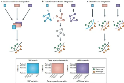
early integration (concatenation based) , late integration (model based) and intermediate integration (transformation based) as depicted in Fig. 1. These integration strategies were initially reported in (Pavlidis et al., 2001) and have been adopted by a number of meta-dimensional analysis studies, for example, protein function prediction (Lanckriet et al., 2004), protein classification (Lanckriet et al., 2003a), gene function prediction (Mostafavi et al., 2008) and protein-protein network inference (Yamanishi et al., 2004).

(a) Early integration or concatenation based approach builds a single model from a single composite dataset formed as a result of combining multiple separate datasets. To achieve this, the individual datasets need to be transformed into a uniform representation. This transformation may also result in a loss of information in certain scenarios (Pavlidis et al., 2001; ˇZitnik & Zu-pan, 2015a). An advantage of this integration strategy is that, once we figure out how to fuse variables into a unified matrix, it becomes relatively simple to analyze continuous and categorical data by using any statistical method.

(b) For late integration or model based approach, training sets derived from multiple data types are used to build separate models.These models created during the train-ing phase are then combined into a unified final model, preserving properties which are data specific.This type of integration strategy is driven by individual hypoth-esis and analysis specific to a particular model and a procedure that combines the resulting models in a meaningful and coherent manner.Although we will be able to analyze each dataset individually using model-based integration, building models in isolation ignores their mutual relationships and therefore can drastically reduce the performance of the final model (Gevaert et al., 2006; ˇZitnik & Zupan, 2015a).

4

Fig. 1. Integration Strategies of meta-dimensional analysis using different data types adapted from (Ritchie et al., 2015): a) Early (concatenation based) integration b) Intermediate (transformation based) integration. c) Late (model based) integration .

integration strategies , with little or no information loss because of non-transformation of data.

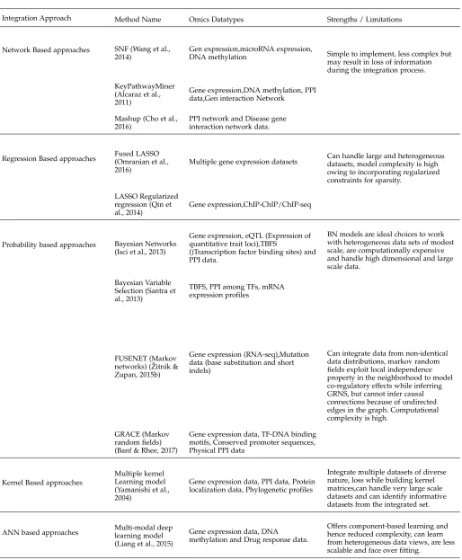
The advantage of building models using a systems ge-nomics approach involves combining multiple data sets of different omics types that can compensate for any missing or unreliable information provided by a single data type. Also genes or pathways that derive their information content from multiple genomic sources are likely to produce less false positives. By considering different levels of genomic, genetic and proteomic regulation, it is highly likely that a near complete biological model can be discovered. A summary of state-of-the art methods used for the inference of regulatory networks is presented in Table 1.

4

N

ETWORK BASED

I

NTEGRATION AND

I

NFER

-ENCE

Network based integration approaches provide the easiest and simplest way to integrate different types of network data into a single unified representation. It is flexible and can handle both homogeneous and heterogeneous datasets. In network data integration lexicon although data types are different, the homogeneous and heterogeneous data are characterized by the similarity/dissimilarity of network nodes. In homogeneous data integration,Nnetworks,Gi=

(V, Ei), with similar vertices (genes, proteins etc.) across

different networks and different edgesEiare combined by

merging edges over the same set of vertices across all the individual networks i,e. Gint = (V, UiN=1Ei) as shown in

Fig. 2.

g1

g3

g2

g4 g5

g6 g7 g4 g5

g6 g7 g1

g3

g2

g1

g3

g2

g4 g5

g6 g7

(a)

(a) (b)(b) (c)(c)

Fig. 2. a) Network1 b) Network2 c) Integrated gene interaction network

Similarity Network Fusion (SNF) (Wang et al., 2014) is a typical example of constructing merged networks by em-ploying homogeneous network data integration principal. SNF that integrates expression data (mRNA, miRNA) and DNA methylation data, creates a network for each data type and then builds an integrated network from the fusion of individual homogeneous networks. The initial steps of the SNF build data set specific similarity matrices. These matrices are equivalent to similarity networks where nodes are genes/miRNA and the weighted edges represent pair-wise node similarities. This is followed by a network fusion step that iteratively builds a single integrated network by employing message passing theory based techniques. The advantage of this iterative network construction is that low

TABLE 1

An overview of integrative approaches that can be employed to infer Gene Regulatory Networks from multiple Omics datasets.Details regarding these approaches are described in separate sections

Integration Approach Method Name Omics Datatypes Strengths / Limitations

Network Based approaches SNF (Wang et al., 2014)

Gen expression,microRNA expression,

DNA methylation Simple to implement, less complex but may result in loss of information during the integration process.

KeyPathwayMiner (Alcaraz et al., 2011)

Gene expression,DNA methylation, PPI data,Gen interaction Network

Mashup (Cho et al., 2016)

PPI network and Disease gene interaction network data.

Regression Based approaches Fused LASSO_{(Omranian et al.,} 2016)

Multiple gene expression datasets Can handle large and heterogeneous_{datasets, model complexity is high} owing to incorporating regularized constraints for sparsity.

LASSO Regularized regression (Qin et al., 2014)

Gene expression,ChIP-ChIP/ChIP-seq

Probability based approaches Bayesian Networks (Isci et al., 2013)

Gene expression, eQTL (Expression of quantitative trait loci),TBFS

()Transcription factor binding sites) and PPI data.

BN models are ideal choices to work with heterogeneous data sets of modest scale, are computationally expensive and handle high dimensional and large scale data.

Bayesian Variable Selection (Santra et al., 2013)

TBFS, PPI among TFs, mRNA expression profiles

FUSENET (Markov networks) ( ˇZitnik & Zupan, 2015b)

Gene expression (RNA-seq),Mutation data (base substitution and short indels)

Can integrate data from non-identical data distributions, markov random fields exploit local independence property in the neighborhood to model co-regulatory effects while inferring GRNS, but cannot infer causal connections because of undirected edges in the graph. Computational complexity is high.

GRACE (Markov random fields) (Banf & Rhee, 2017)

Gene expression data, TF-DNA binding motifs, Conserved promoter sequences, Physical PPI data

Kernel Based approaches

Multiple kernel Learning model (Yamanishi et al., 2004)

Gene expression data, PPI data, Protein localization data, Phylogenetic profiles

Integrate multiple datasets of diverse nature, loss while building kernel matrices,can handle very large scale datasets and can identify informative datasets from the integrated set.

ANN based approaches Multi-modal deep_{learning model} (Liang et al., 2015)

Gene expression data, DNA methylation and Drug response data.

Offers component-based learning and hence reduced complexity, can learn from heterogeneous data views, are less scalable and face over fitting.

weight (weak) edges exclusive to all component networks are discarded in order to remove noise and high weight

6 integrated are not discarded depending on how densely

connected their network neighborhoods are across the net-works. With such non-linearity SNF makes full use of the local network structure, combining common as well as com-plementary information of the structure across networks. Similarly, using this principle, multi omics data of cohort features can be integrated for the reconstruction of gene regulatory networks (GRNs), for example, given multiple RNA-seq/ micro-array datasets generated under different perturbations/ treatments/condition can be used to learn multiple Gene Regulatory Networks (GRN) from ech data set, we can then use SNF to fuse these individual GRNs into an integrated GRN. Similarly, GRNs inferred using al-gorithms, such as, CLR (Faith et al., 2007),ARACNE (A. Mar-golin et al., 2006), SIRENE (Mordelet & Vert, 2008) can also be fused by a method like SNF to achieve robust results, which implements the philosophy - ‘the wisdom of crowds‘ (Marbach et al., 2012). A similar network fusion method has been proposed in KeyPathwayMinerWeb for pathway enrichment analysis using multi omics data (Alcaraz et al., 2011).

Another study by (Gade et al., 2011) builds a transcrip-tional regulatory network of prostate cancer from mRNA and miRNA expression profiles. Besides these two data sets, their method also incorporates prior knowledge about miRNA targets from MicroCosm (Enright et al., 2003) target database. Here the authors start by building a bipartite graph connecting miRNAs mij to their respective mRNA mi targets. These relationships are established by

comput-ing Pearson correlation coefficients between the expression vectors of both mRNA and miRNAp(mi, mij)resulting in

p-values form every mRNA-miRNA pair .

Besides the mRNA-miRNA pair, p-valuesP_i,jpredfor tar-get predictions from the MicroCosm database (Enright et al., 2003) are included as a secondary source of information. Incorporation of this predicted information strengthens the confidence of relationship between a mRNA and miRNA when some supportive information is provided from the available biological data. MicroCosm database generally stores mRNA-miRNA pairs whose p-values are below 0.05, in case the pair does not exist in database then the value is set to 1.

pcor_i,j =P(H0: (mi, mij) = 0)

∀i∈1, p1, j∈1, p2

(1)

P-values from both the sources (mRNAs & miRNAs) are combined using truncated product method (Zaykin et al., 2002) to yield a weight matrixWi,jviewed as adjacency

ma-trix, describing relationships between mRNA and miRNA using a bipartite graph. The resultant graph W has edges from mRNA to miRNA and is interpreted as a directed graph. Although the study was not primarily designed to infer a regulatory relationship between mRNA and miRNA, but as a pre-requisite to identify prognostic signatures that are able to predict clinical outcome in prostate cancer. The results of the study clearly indicate an improvement in pre-diction performance with graph incorporated as regulatory information. Also introduction of likelihood-based boosting in (Binder & Schumacher, 2009) as a possibility to integrate gene interaction network into feature selection improves the predictive performance of the model.

The heterogeneous network integration method uses simple projection techniques to combine different types of vertices and edges across a number of networks. This type of network integration is usually done for association studies, for example, network projections of gene-gene interaction (GI) on a disease similarity network (DSN). Also projecting GI network on to a disease association network disturbs the GI network structure resulting in loss of information carried by the GI network. More sophisticated methods based on diffusion (information flow across network connections) overcome the projection based integration. The diffusion process explores the structure of each network and their corresponding mutual relationships in order to infer an integrated network. These approaches fall under the domain of network propagation methods and have been applied to a variety of biological problems, such as drug-target prediction and drug re-purposing (Cheng et al., 2012), drug-disease association (Huang et al., 2013) and gene-drug-disease as-sociation (Guo et al., 2011). Another important study in this direction was carried out by (Cho et al., 2016) that led to the development of integrative framework called ’Mashup’.The Mashup framework exploits the topological representation of individual networks, analyzing each network separately by running a localized network diffusion algorithm, random walk with restart (Tong et al., 2006) to obtain the distribution of each node and their relevance to other nodes in the network. These feature vectors are then used as input by the framework to carry out mutiple tasks, such as gene interaction and gene function prediction etc.

More recently heterogeneous network integration ap-proaches are being used for building Drug-target interac-tion networks in order to identify new indicainterac-tions for the old drugs (drug re-purposing). DTINet, a computational pipeline developed by (Luo et al., 2017)combines diverse information from heterogeneous networks by integrating a dimensionality reduction technique, DCA (diffusion com-ponent analysis) with a network diffusion algorithm RWR (random walk with restart) in order to obtain low dimen-sional feature vector representation of the network nodes, a process known as compact feature learning.This feature vector embeds relational properties (e.g. similarity), associ-ation informassoci-ation and topological informassoci-ation of each drug (or protein) node in the heterogeneous network.

5

R

EGRESSION

B

ASED

A

PPROACHES

genes is decomposed intoP regression problems and tree-based ensemble methods using either Random forests or extra-trees are used to predict the expression pattern of target genes from the expression profile of all other input genes. A putative regulatory link between the input gene and its target is predicted based on the role played by the in-put gene in the prediction of target gene expression pattern. Links from all the genes are ranked and then aggregated to reconstruct a GRN.

In summary, although performance of regularized re-gression models in GRN inference compared to other ap-proaches yielded better results, an increase in accuracy was observed in (Qin et al., 2014) when the authors in-tegrated ChIP-ChIP/ChIP-seq data in the form of prior knowledge usingLp(P <1)i,e.P0, P1/2 regularization. In (Chartrand, 2007; Z. Xu et al., 2012), regularization models

Lp(P < 1) have been reported to perform optimally even

on data with fewer samples and achieved higher sparsity and more accurate solutions.SinceL0 and L1/2 regression models suffer from non-convexity, therefore iterative hard and half thresholding algorithms are used to solve these models (Fornasier & Rauhut, 2008). The advantage with these algorithms is that, they have a low computation cost and a fast convergence rate, both essential properties worth consideration while designing algorithms for genomic scale data.

5.1 Lpregularization models

A linear system representation of relationships between tar-get genes and their regulatory proteins (TFs) can be written

as:-AX=B+ (2)

Here A ∈ Rm×r represents a matrix containing gene expression values of candidate TFs , B ∈ Rm×n _{is the}

matrix containing gene expression values of target genes,

∈Rm×n

is the error matrix andX ∈Rr×n

is the target-TF regulation matrix,mandrrepresent the matrix dimen-sion and number of TFs respectively while n is the total number of target genes. The objective here is to minimize the difference betweenAXjandBj with few TFs, a sparse

optimization problem, which can be written as

:-kAXj−Bjk2

s.tkXjk0≤K

(3)

Where k.k denotes the Euclidean norm as kXjk2 = pPr

i=1Xi,j2 and kXjk0 denotes the number of non-zero elements in Xj and less kXjk0 means higher sparsity of

Xj, an indicator of number of TFs found to be responsible

for regulating the target genej.

For solving such inference problems , the practical ap-proach is to transform the sparse optimization problem into a regularization problem. For example , with Bj as the

expression profile of a given gene j, theL0 regularization model imposes a minimization constraint on the difference betweenAXjandBjand a maximization constraint on the

sparsity ofXjas given by :

min

Xj∈Rr

kAXj−Bjk22+λkXjk0 (4)

where regularization parameterλ >0provides a trade-off between sparsity and accuracy.L0regularization is very close to our initial probelm, but solving it to achieve a global optimal solution is NP-hard, therefore a relaxation ofL0,L1 (LASSO) regularization is introduced to solve

it:-min

Xj∈Rr

kAXj−Bjk22+λkXjk1 (5)

where kXjk1 = Pri=1kXi,jk. In many instances , the

solutions obtained using LASSO (L1) model are less sparse than theL0regularization.

Recently , L1/2 regularization has been proposed and has been shown to perform better than LASSO (L1) regular-ization (Z. Xu et al., 2012).This model is described as

below:-min

Xj∈Rr

kAXj−Bjk22+λkXjk

1/2

1/2 (6)

wherekXjk

1/2 1/2= (

Pr

i=1kXi,jk)2

Qin et al. applied iterative thresholding algorithms to solveL0,L1/2andL1regression models. For example,L1 models are solved using iterative soft thresholding algo-rithms andL0andL1/2regression models use iterative hard and half thresholding algorithms for obtaining optimum solutions. These iterative algorithms are computational very efficient with fast convergence rate and effective tools for handling large scale sparse optimization problems. A de-tailed discussion on iterative thresholding algorithms can be found in (Fornasier & Rauhut, 2008).

Regularization parameter λfor all the thresholding al-gorithms is updated iteratively to maintain the sparsity of

X_jk. All the three regularization models were evaluated on mESC (mouse embryonic stem cell) data set. The ini-tial experiments were performed on transcriptomic data alone and compared with TF-target datasets from high throughput (microarray/ChIP-X) and low throughput (lit-erature curated). Both these TF-target datasets serve as gold standard against which the model accuracy is tested. The ROCs of all the models on both evaluation data were close to random with transcriptome only dataset. However, on the integration of the chip-X data into the models , it was observed that the performance of all the models improved drastically withL0andL1/2models significantly outperforming L1 regularization model. ROC of all three regression models Lp(p = 0,1/2,1) are high with high

throughput gold standard and low with low throughput gold standard. At an FPR of 0.05, the integrated models yield a TPR of 0.63, 0.59 and 0.07 forL0, L1/2andL1models, while transcriptome only models achieve 0.03, 0.03 and 0.04 TPR. They demonstrated thatL0, L1/2 models achieve higher sensitivity with integrated chip-X data compared to transcriptome only dataset.

Another regression based study that infers gene regu-latory networks used Fused LASSO to integrate multiple transcriptomic datasets subject to different perturbations (Omranian et al., 2016). The approach formulated by authors combinesL2norm (residual sum of squares) withL1(sum of absolute values of regression coefficients), shrinking coef-ficients and yielding sparsity as the coefcoef-ficients approach towards zero. Unlike LASSO where the minimization of

8 difference of the regression coefficients of corresponding

regressors (Tibshirani et al., 2005).Further, the fused LASSO formulation has been extended here by incorporating infor-mation about regressors and response genes based on the similarity of their differential behavior. To ensure that the inferred networks are sparse, the fusion approach imposes a similarity constraint on the inferred relationships from each dataset with biologically meaningful evidence. Since this approach relies on similarity of the differential behavior, the model operates on P regressor genes and a single gene as a response gene, multiple gene expression datasets represented byXi, obtained underKdifferent experimental conditions along corresponding controlsXc,i _{(1 ≤ i ≤k),}

and the expression profiles Yi

for response genes along corresponding response control profiles Yc,i over k con-ditions (1 ≤ i ≤ k) are used to obtain condition specific differential behavior of regressors and response genes. The differential behavior thus obtained is used to calculate the weight matrix denoted by Wi

P×P from the probability of

differentially expressed regressorP ri,t_j and response genes

P r_Yi,t which capture the similarities between each of the regressor and response gene at time point t is given by:

W_Y,ji = 1

N N

X

i=1

|P ri,t_Y −P ri,t_j | (7)

5.2 Regression model for fused LASSO

For efficient inference of GRNs, the regression model formu-lated in equation (8) is based on three fundamental criteria:-1) Obtained regression should be sparse to ensure less false positives and high likelihood of detecting direct relationships. Biologically , the expression level of a few TF coding genes should explain the expression level of their presumed targets.

2) For effective explanation of the analyzed condition, the model should infer the regulatory network from all k datasets simultaneously.

3) Genes exhibiting similar differential behavior are prof-fered while assigning direct regulatory links.

While LASSO captures the first criterion, the second criterion of inferring regulatory networks from all datasets can be achieved by imposing the LASSO penalty simulta-neously on all the integrated and transformed datasets. k

transcriptomic datasets are clubbed together to form a single block matrix X denoting expression profiles for P genes , while as vector Y is response expression profiles over

k different conditions The reconstructed networks should be evaluated for proximity in terms of their interaction strengths given by regression coefficients that correspond to links among the responseY and regressor genesXin the

knetworks.This vector is represented asβ.

For reconstructed networks to be in close proximity to each other, the final model includes a fusion termkβ00−β0k, whereβ0 = [β1_{, β}2_{, ...., β}k−1_]T

and β00 = [β2_{, β}3_{, ...., β}k_]T

.This term is included to impose a minimization constraint for the sum of absolute differences among the estimated regressor coefficients over multiple datasets. Within the fused LASSO formulation the inclusion ofWi (1 ≤i ≤k) implies the similarity of the differential behavior between

response and the regressor genes. This matrix multiplied with the regression coefficients ensures that the regres-sors having high explanatory powers and associated with non-zero coefficients and are less penalized over multiple datasets.Therefore the expression kW βk1 is added as an additional penalty in the proposed regression model. For reconstruction of gene regulatory network interactions an final model over k given datasets is given

as:-ˆ

β =argmin

β kY −Xβk

2

2+λ1kW βk1+λ2kβ00−β0k1 (8)

Here regressors whose regression coefficients shrink to-wards zero are the potent regulators of the response gene

Y. A comparative analysis of this approach with other state of the art methods viz, global silencing (Barzel & Barab´asi, 2013), network deconvolution (Feizi et al., 2013), Gaus-sian Graphical Models (GGM)(Sch¨afer & Strimmer, 2004; Kr¨amer et al., 2009; Chun et al., 2013), mutual information (ARACNE and CLR) (A. A. Margolin et al., 2006; Faith et al., 2007; Zoppoli et al., 2010) (Meyer et al., 2007), Bayesian Networks (Friedman et al., 2000), the GENIE3 (Irrthum et al., 2010) approach and other regularization based models is performed using network sparsity and removal of the indirect relationships as dual criteria for model evaluation. The GGM,ARACNE and CLR perform poorly for accurate inference of regulatory networks, on the contrary, fused LASSO approach in addition to retrieving the regulatory links efficiently also predicted the type of regulation (ac-tivation/repression), therefore outperforming most of the contending methods on the set criteria.

6

P

ROBABILITY

B

ASED APPROACHES

6.1 Bayesian Networks

Bayesian networks (BNs) or belief networks as they are often called belong to the family of probabilistic graphical models used to represent knowledge about an uncertain domain. These networks are represented using directed acyclic graphs (DAGs), wherein each node represents a random variable and the edges between the nodes represent the causal connections / probabilistic dependencies among the corresponding random variables (Ben-Gal et al., 2007). These conditional dependencies are estimated by using sta-tistical and computational methods .Therefore BNs combine principles from graph theory, probability and statistics.

Bayesian networks are recognized as important tools in data driven biological science research and play a pivotal role in performing several biological tasks such as infer-ring cellular networks (N. Friedman, 2004), data integra-tion (Troyanskaya et al., 2003; Santra, 2014), classificaintegra-tion (Bradford et al., 2006) and genetic data analysis (Beaumont & Rannala, 2004).

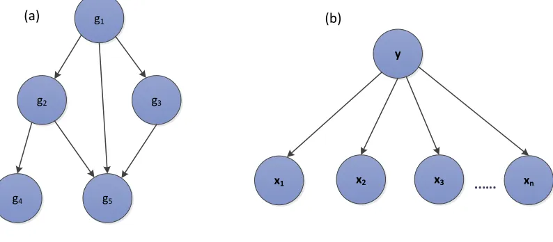
The graphical representation and use of probabilistic formalisms make BNs suitable for combining data and domain knowledge, express causal relationships, learn from incomplete datasets and provides a natural setting for modeling stochastic nature of biological systems and its measurements. The graph in Fig 3(a) provides an example a BN describing a gene regulatory network. This network represents a joint probability distribution (JPD) over a set

g1

g2 g3

g5 g4

y

x1 x2 x3 ..…. xn

(a) _(b)

Fig. 3. (a) A graphical illustration of Modeling of Gene Regulatory Network using BN. Vertices denote the genes whereas the directed edges represent the regulatory relations between the genes.Here Geneg1regulates the expression ofg2,g3 andg5, genesg2andg3also regulateg5, whereasg4is only regulated byg2.(b) Graphical depiction of anaive BNwith class nodeyacting as parent to independent nodesx1, x2, x3....xn.

of random variables V, depicted as an annotated acyclic graph. The pair B= (G, Θ), where G is the DAG whose nodes represent genes as random variablesg1, g2, g3, ..., gn

and whose edges represent direct dependencies between the genes. The other component of the network Θ is used to represent a set of parameters. Th elements of this set are the parameterθxi|πi =PB(xi|πi)for every realizationxi ofgi

conditioned onπi, set of parents ofXiinG.

The DAG structure embeds conditional independence relationships, i.e. given its parents inG, a nodegidoes not

depend on its non-descendants The JPD defined byB over

V can be written

as:-PB(g1, g2, g3, ....gn) = n

Y

i=1

PB(gi|πi) (9)

Bayesian Networks have been used to build suitable frameworks for modeling and integration of different types of biological data. Network inference from disparate data is one of the biggest challenges in the field of systems biology, sparse network construction containing important gene associations (strength of this relationship within the network is represented by conditional probabilities in a joint probability distribution). Constructing a BN that provides an effective description of our data involves two important steps: structure learning and parameter learning. (Needham et al., 2007; Ben-Gal et al., 2007). Because the possible number of BN structure grows super exponentially with the number of nodes , the problem of finding a BN with best description of data is Np-complete, therefore heuristic methods have been employed for solving such problems (Chickering, 1996).

Studies employing bayesian networks for integrating gene expression data with other genomic datasets in a het-erogeneous data integration framework have widely been reported in the literature.For example, (Zhu et al., 2008) built a probabilistic causal yeast regulatory network by combining gene expression data(GExD), transcription factor binding site (TFBS), eQTL(Expression of quantitative trait

loci) and PPI data using bayesian learning .While testing the performance of constructed BN, they demonstrated an integrated BN model possesses higher predictive power than a BN model derived from single data type (gene expression data).A similar approach to construct a proba-bilistic model for GRN inference from brain tissue of late-onset Alzheimer’s has been adopted by (Zhang et al., 2013) by integrating patient data .

Earlier studies of data integration using BNs has been reported in (Gevaert et al., 2006) to predict the outcome of breast cancer from heterogeneous genomic datasets. They constructed the BN network in order to classify the patients into different prognosis groups (good/poor).They increased the performance of the BN by subjecting it to all the three integration strategies as described above and observed that intermediate strategy was the one with improved results.Another study from (Van Vliet et al., 2012) using multiple classifiers with varying complexity also concluded in favour of intermediate integration.

Most of the data integration studies for heterogeneous biological data have used Naive Bayes (simple BN) for constructing integrated networks from genomic datasets, such as gene-gene association network (Lee et al., 2004; Linghu et al., 2009; Franceschini et al., 2012; Jansen et al., 2003). Here all independent nodes representing heteroge-neous data sources are treated as child nodes of a class node, such simplicity in Bayesian Network structures enable efficient learning and much faster inference approaches. For example, gene-gene association studies use naive BN structures for prediction purposes where class nodes rep-resent a set of proteins/genes (interacting/non-interacting) while independent nodes represent multiple data sources.A graphical depiction of naive baye’s is shown in Fig 3(b).

10 as the effect of perturbation rapidly propagates through

the entire network.This premise has been shown to be true through the works of (Rogers & Girolami, 2005; Lo et al., 2012). They have shown that the response expressionxi_of

target genes (gi) are linearly dependent upon the response

expression Xi_{of their direct regulators g}i _{against a set of}

perturbations (np).

xi=XiTβi (10)

Where βi _{are the linear coefficients representing the}

type and strength of interaction between genes (gi) and

its direct regulators (gi). Since no perturbation experiments are error free, therefore measurements of the expression levels are always accompanied by some sort of noise called ’”residuals’”. To accommodate these residuals in the linear model, the above equation now

becomes:-xi=XiTβi+i (11)

where i is the residual error and a linear combination of these variables (i) denotes total noise of individual

measurement errors (Kariya & Kurata, 2004) that the per-turbation responses of the genes (gi) and their regulators

(gi_{)are associated with.}

In order to find the direct regulators (gi_{) of the gene}

(gi), the requirement is to calculateβiin least square sense.

In this formulation , the task of identifying the direct reg-ulators gi _{of target genes g}

i is determined by the values

of βi_{. Elements (β}

ik, k = 1, ..., np) of βi whose values

are > 0 are chosen as significant direct interactions and therefore the direct regulators of genesgiare corresponding

genes gk.Performing perturbation experiments on a large

scale is neither feasible nor possible under most of the circumstances. Hence in such situations reconstructing a full network is not possible and the problem can be resolved by Bayesian variable selection (BVS) algorithm (Santra et al., 2013).

In BVS formulation an adjacency matrixAis used to rep-resent a GRN topology, elements of the matrix with non-zero valuesAikdenote a direct regulatory relationship between

genesgiandgk,(k 6=i), on the other hand elements with

zero values represent no direct regulation. There is a close relationship between elements in matrixAand the elements of matrix interaction strength β.Given two genes (gi, gk),

absence of direct interactions (Aik = 0, k 6= i) between

them implies a zero interaction strength (βik = 0, k 6= i),

in β and vice versa. Hence, to locate direct regulators of a genegiwithin the binary adjacency matrix is equivalent to

locating elements ofAin theithrow of the adjacency matrix whose corresponding strength of interaction inβis not zero. Since it is computationally inefficient to iterate across all the combinations of Ai_{, BVS algorithm adopts a Bayesian}

approach to avoid the iteration process. The Bayesian algo-rithms learns in a more natural way, the knowledge updates for some events is carried out only as the new information becomes available.In bayesian lexicon, prior distributions are used to encode the information about certain events and hence assigning a prior probability to each possible outcome of the event (Heckerman, 1998).

For GRN inference the prior distribution (P(Ai)) en-codes the prior knowledge about gene gi and its direct

regulators gi_{.In (Santra et al., 2013), the model does not}

use any prior knowledge and the approach favors sparsity, penalizing models with too many regulators. Here, a more informative prior distributionAi_{is injected into the model}

using integrated TFBS data and PPI data among TFs. The application of BVS algorithm was demonstrated by reconstructing a liver specific GRN by using perturbation data. Different prior distributions were tested for model

evaluation:-1) Prior distribution ofAi was formulated without using any prior knowledge from an external data source. 2) Although no prior knowledge is incorporated , the

prior distribution was tailored to favor sparse regula-tory programs.

3) A prior distribution ofAi_{was formulated based on the}

predicted information about direct regulatory interac-tions from publicly available TFBS data.

4) Both direct and indirect regulatory interactions were used to construct a prior distribution ofAi _{from TFBS}

data and PPI data between TFs.

To estimate the posterior probability of interactions, the BVS algorithm uses Markov Chain Monte Carlo (MCMC) sampling strategy. The probabilities thus obtained represent the confidences on each interaction based on the perturba-tion responses. An interacperturba-tion is considered to be true if the probability is above a certain threshold (Pth) and absent

in case the probability is below or equal to the threshold (Pth).GRNs reconstructed from the true interactions are then

compared with the gold standard.

Results of BVS formulation were compared with LASSO based algorithms using different prior settings.The first case does not use any prior and the regularization parameter

λ1 is set to 0.2. In case of second and third setting a prior distribution of TFBS and TFBS+PPI with regularization pa-rameters set toλ1 =0.2 andλ2=0.8 respectively. Evaluation with ROC and PRE curves suggests that with the inclu-sion prior information, the performance of BVS algorithm improved significantly. Prior knowledge about direct and indirect regulatory interaction from TFBS integrated with PPI data between TFs were observed to improve predictive-ness of regulatory relationships than the TFBS data alone. More over, the proposed BVS formulation outperformed all LASSO models in all circumstances.

Modeling using BNs provides an efficient and suitable framework for integration of multiple datasets (homoge-neous/heterogeneous). They are able to capture noisy ditional dependencies between data variables and the con-struction of CPDs makes them suitable for a variety network inference problems in bioinformatics.However, there are certain limitations of BNs as well:

i Although some important associations are captured using the sparse network representation, some of the associations may be missing in the final network. ii Network loops which in many biological networks

represent important control mechanisms can not be inferred using BNs because of their acyclic nature. iii As the number of nodes in the model increase, BN

structure grows exponentially with a huge computa-tional cost, therefore making BNs less attractive for large scale studies ( e.g. eukaryotic genomes).

6.2 Network inference through Markov networks

Graphical probabilistic models with undirected edges are called Markov networks.These networks provide a simple definition of independence between any two nodes and are used to represent conditional dependence relationships between genes. Mechanisms within the biological cells are governed by complex interactions among various genes and it would be of great interest for biologists to understand the conditional dependencies between these genes. It is possible to uncover these dependencies from the experimental data characterizing genes and gene products and represent them in the form of a gene network. Markov networks present a popular statistical approach to model such conditional independence relationships in high-dimensional genomics data. In particular the absence of a link between genes s and t is indicative of independence relationship between s and t, considering the immediate neighborhood of s. From (Murphy, 2012) with such properties we can conclude that, two nodes (genes) without any direct links between them are conditionally independent of each other given the rest of the genes in their vicinity. Such a property of condi-tional independence (Markov) allow existence of a rich set of dependence relationships between nodes and therefore, we can uncover complex relations among the nodes of a Markov network (Allen & Liu, 2013).

The problem of learning network structures using Markov networks have witnessed wide acceptance from the fields of computer vision (S. Z. Li, 1994), social networks, image and signal processing (C. Wang et al., 2013; Metzler & Croft, 2005) and genomics (Wei & Li, 2007). The applica-tions of undirected graphical models (Markov networks) in bioinformatics include construction signaling network for cancer from proteomic data (Mukherjee & Speed, 2008), genetic interaction network reconstruction from integration of multiple datasets (Isci et al., 2013) and in recent times various inference algorithms based on Markov networks using NGS data have been developed (Allen & Liu, 2013; Gallopin et al., 2013).

ˇ

Zitnik and Zupan developed FUSENET ( ˇZitnik & Zu-pan, 2015b) as a GRN inference algorithm based on Markov network formulation that integrates multiple non-identically distributed heterogeneous datasets. The input to FUSENET is a dataset colletion with each dataset containing a set of gene expression profiles. Gene expression measure-ments are taken from RNA-seq experimeasure-ments (discrete, non-negative) and are combined with mutation data including CNV, SNP, short indels and multiple substitutions. While the RNA-seq data follows Poisson or negative binomial distribution, the data from mutation datasets are modeled either using categorical or multinomial distributions . A prominent feature in FUSENET is the latent factor rep-resention of model parameters. Employing latent factors and the flexibility to share these factors across different datasets makes it easy for the algorithm to perform network inference tasks from multiple datasets considered simalta-neously and arising from different probability distributions. The network model offered by FUSENET offers a collective approach to inference, whereby the network estimation is performed jointly from non identical data distributions.The FUSENET model is illustrated as below:- Given a collection

s1

s2

s3

s4

s5

s6

s7

S2 S3 | {S1, S4}

Fig. 4. A Markov network modeled using FUSENET, that infers depen-dencies among any two genes conditioned on their neighbors. Here dotted line denotes an absence of edge betweens2 ands3 implying thats2acts indepent ofs3given its neighbourss1ands4. The⊥symbol stand for conditional independence.

D of n observations, D = {x1_{, x}2_{, ...., x}n_}

where xi

is a p-dimensional vector drawn from a specific probability distribution. This distribution is associated with a graph

G = (V, E∗) with parameters{θ∗_c, c ∈ C}. Because Graph G embeds the Markov independence properties among the nodes, therefore the task of reconstructing the topology of G is to infer an edge E∗ corresponding to the probability distribution where from the initial observations in D were drawn.Therefore set of edges as a function of parameters can be written

as:-E∗={(s, t)∈VxV:∃ clique c∈C:

{s, t} ⊂c∧ {θ_c∗6= 0}} (12)

Learning the structure of network using FUSENET there-fore aims at estimating the weights{θ, cˆ ∈_C}whose values should possibly close to the true but otherwise unknown parameters {θ_c∗, c ∈ _C}.For the final model to take shape, authors chose a pairwise Markov network with joint proba-bility distribution model having cliques of size at most two:

P(X)∝exp

X

s∈V

θ_s∗B(Xs)

| {z }

setof nodes

+ X

(s,t)∈V xV

θ∗_stB(Xs)B(Xt)

| {z }

setof edges

+X

s∈V C(Xs)

(13) with entries θ∗st 6= 0 if t ∈ N(s) and θ∗st = 0 if t /∈ N(s).The overall Markov network structure is then estimated by adopting neighborhood estimation approaches following the works of (Ravikumar et al., 2010; Jalali et al., 2011; Allen & Liu, 2013), the estimate for the entire network

ˆ

Eis then obtained using :

ˆ

E = [

s∈V,t∈_Nˆ_(s) n

(s, t)

o

12 where (s, t) represent an edge between nodes s and

t and Nˆ(s) = {t ∈ V\{s} : ˆθst 6= 0} is the

esti-mated neighborhood of node s. In order to assess the performance of FUSENET, several competing inference al-gorithms were considered. The FUSENET model was com-pared with both Gaussian and non-Gaussian models in-cluding Graphical LASSO (J. Friedman et al., 2008), Local Poisson Graphical Model (LPGM) (Allen & Liu, 2013) and Multinomial Morkov Graphical Model (Mult-GM) (Jalali et al., 2011) for performance evaluation. The considered inference methods along with FUSENET were applied to Poison-distributed simulated data.Four network types viz. random, hub, small world and scale free were generated , the last three being characteristic of many real biological networks. Datasets havingP = 100(nodes) variables and

withn= 200observations were generated. ROC curves for

all the simulated networks using comparative and proposed methods were reported. It was concluded that FUSENET outperforms Gaussian based competitors (GLASSO, Log-GLASSO) as well as methods modeled using Poisson data (LPGM,Mult.GM).This shows an overall and consistent per-formance of FUSENET across all considered networks and more than one data distributions.For in depth understand-ing of the model refer( ˇZitnik & Zupan, 2015b)

Since GRN inference for most of the eukaryotic organ-isms remains a challenging task, another important study by (Banf & Rhee, 2017) using Markov random fields exploits the prior biological knowledge and heterogeneous data in-tegration to build high confidence network prediction mod-els.The study uses two datasets to evaluate the prediction accuracy of the proposed algorithm. One of the findings on A.Thaliana dataset is covered here. For reconstruction of a GRN, data from three different sources were integrated.(i) A conserved non-coding sequence 2000bp promoter region of 17610 genes,(ii) DNA binding predictions within these sequences for 120 TFs and (iii) gene expression dataset of A.Thaliana development, comprising RNA samples from 83 tissues.This data was used to derive a condition specific co-expression network.A variance based filtering was applied to remove genes that exhibit little variance across all tissues and development stages.

For network inference, a highly robust and scalable tree based regression which decomposes the network inference into separate regression problems for each target gene, this model calculates an important measure for each predictor, which is used as an indicator for a link to be present between the regulators and target gene. Given a large number of regulators in A.Thaliana , Banf & Rhee (2017) computed ran tree based regressions with more than 5000 decision trees for each target gene to ensure that regulators are selected multiple times during bootstrap aggregation so as to provide stable prediction for each target gene. For all the evaluations, they retained all the predictions beyond 95th

percentile of the distribution.

Given a set of regulatory links l, there is a concept of meta gene regulatory networks that describes connections between two linkslandl0i.e.,l↔l0. A connection between two links l, l0 is based on the co-regulation principle i.e., two different target genes g and g0 are controlled by the same regulatorr.

l↔l0=r→ {g, g0} (15)

The weight of such a connection is based on a distance metric that combines two measures which are assumed to reflect co-regulation.Given this meta gene regulatory network, modules of connected regulatory links can be extracted from the meta network.Each module represents a group of large genesgthat are pair-wise co-regulated by a specific TF r. Individual links that are not connected to any other link are also retained as individual (single link) modules.The co-regulatory effects within each module are modeled using Markov random fieldsG = (V, E), which implements a local independence assumption referred to as Markov property (Schwaller, 2015). This property imposes a node to be independent of any other nodes given all its in direct neighbors, i.e.:

∀i∈V, Xi⊥XV −i|XNi (16)

Where Ni, j|{i, j} ∈ E denotes the set of immediate

neighbors of nodeVi.An important notion in the model is

a clique. It is defined as fully connected subset of nodes within the graph, which is considered as maximal if it is not connected within any other larger clique.In order to retain the links in the final network , the model favors links with high weights as well as strongly connected pairs of regulatory links to be in the same state.

7

K

ERNEL

B

ASED

A

PPROACHES

Kernel methods represent a mathematical framework which embeds data points (genes, proteins, miRNA etc) from input spaceIto feature spaceFby employing a kernel function. Genomic datasets viz., mRNA expression levels from RNA-seq, miRNA expression profile from miRNA-seq and TF-gene regulation matrix obtained from different databases such as ENCODE (E. P. Consortium et al., 2004), TRED (Jiang et al., 2007), TRRUST (Han et al., 2015) etc. comprise heterogeneous datasets that serve as the building blocks of gene regulatory networks which can be fused together using kernel methods.

Each dataset is transformed into a symmetric positive semi definite kernel matrix by means of a kernel function, that is a real valuedk(x1, x2)satisfyingk(x1, x2)=k(x2, x1) for any two objects x1 and x2 and positive semi-definite i.e., to say Pn

i=1aiaj k(xi, xj) ≥ 0 for any integer n, set

of objects (n = x1...xn) and any set of real numbers

(a1...an)(Charpiat, 2015). Kernel functions provide a

co-herent representation and a mathematical framework for the input data (genes, TFs, miRNA etc.) and represent the object features via their pairwise similarity values comprising the n x n kernel matrix, defined as.

K=



    

k(x1, x1) k(x1, x2) .. k(x1, xn) k(x2, x1) k(x2, x2) .. k(x2, xn)

. . .. .

. . .. .

k(xn, x1) k(xn, x2) .. k(xn, xn)



    

(17)

Kernel methods offer a modular approach to pattern analysis (Shawe-Taylor & Cristianini, 2004). An algorith-mic procedure is devised together with a kernel function

that performs an inner product on the inputs in a feature space. This algorithm is more generic and can work for any kernel and hence for any data domain. The kernel part is data specific that offers an elegant and flexible approach to design learning systems, that can easily operate in very high dimensional space. It is a modular framework, where modules are combined together to obtain complex learning systems. Some examples of commonly used kernels are (Shawe-Taylor & Cristianini, 2004):

Linear kernel

Φ(x1)TΦ(x2) =x1Tx2=k(x1, x2) (18)

Polynomial kernel

k(x1, x2) =hx1, x2id (19)

Gaussian kernel

k(x1, x2) =exp

−kx1−x2k

2−σ2

(20)

For suitable values of d (degree of the polynimial kernel) andσ (spread parameterof gaussian kernel), the similarity measure k(x1, x2) between x1 and x2 is always positive with is maximum atx1 = x2. All pointsxhave same unit norm (sincek(x1, x2) = 1∀x) suggesting that images of all points in x lie on the unit sphere inH(Sch ¨olkopf & Smola, 2002).

In order to handle genomic datasets like DNA sequences , protein sequences and network data such as, protein-protein interactions, molecular and cellular networks, cus-tomized kernel functions have been proposed for build-ing similarity matrices. For example,kernel functions for computing the similarity between two genes/proteins are spectrum kernel (C. Leslie et al., 2001; C. S. Leslie et al., 2004) , pairwise kernel (Ben-Hur & Noble, 2005) , motif kernels (Ben-Hur & Brutlag, 2003) for defining similarity between TF-DNA binding motifs (Ben-Hur & Brutlag, 2003), and pfam kernel (Gomez et al., 2003). Network data represented using adjacency matrices is transformed into a similarity matrix using diffusion kernel.For more in depth coverage on range of kernels devised for handling biological data refer to (Sch ¨olkopf et al., 2004).

Besides the sequence data that normally occurs in string format, network data from molecular networks and inter-action networks, pathways and Gene Ontology (GO) as-sociations are frequently used in kernel based integration studies. These types of datasets can be handled using graph with different scenarios. In the first case,the input varibales can be treated as nodes within a graph,e.g. proteins in PPI networks or genes in case of GRNs and in the second scenario proteins can be represented using graphs, e.g. protein representation using phylogenetic trees. Computa-tional biologists have developed kernels for both scenar-ios. For example, kernels built from phylogenetic profiles modeled as trees (Vert, 2002), graphical representation of small molecules (Kashima et al., 2004) and graphs modeling protein structures (Borgwardt et al., 2005).

7.1 Multiple Kernel Learning Model

Multiple kernel learning (MKL) is a paradigm shift from tra-ditional single feature based learning and offers an advan-tage of combining multiple features of objects such as genes,

proteins, metabolites etc., as different kernels (Sonnenburg et al., 2006). This information can be fed as an ensemble into an MKL learning algorithm as a combined kernel matrix for classification or regression tasks on unknown data. The basic algebraic operations of addition, multiplication and exponentiation when performed in combining multiple ker-nel matrices preserves the positive semi-definite property and enable the use of powerful kernel algebra. A new kernel can be defined using k1 and k2 with their corresponding embeddingsΦ1(x)andΦ2(x). This resultant kernel is

K=k1+k2 (21)

with the new induced embedding

Φx= [Φ1(x),Φ2(x)] (22)

Given a kernel setK ={k1, k2, ...., km}, an affine

com-bination of m parametrized kernels can be formed as given below:

-K=

m

X

i=1

µiki (23)

subject to the constraint that µi (weights) are positive i,e. µi ≥ 0, i = 1...m A kernel based statistical classifier

such as SVM induces a margin in feature space, separating the two classes using a linear discriminant.In order to find this linear discriminant, an optimization problem needs to be solved, known as a quadratic program (QP). A Quadratic program is a form of convex optimization problem, which are easily solvable.

Kernel based integration methods were first proposed in (Lanckriet et al., 2004), wherein a 1-norm soft margin SVM is trained for a classification problem separating membrane proteins from ribosomal proteins. They combined hetero-geneous biological datasets viz. PPI,amino acid sequences and gene expression data, characterizing different proteins by transforming them into multiple positive semidefinite kernel matrices using different kernel functions.Their find-ings reveal an improved classifier performance when all datasets are integrated as a unit compared to testing the classifier on individual datasets. In an earlier study on function prediction for baker’s yeast proteins (Lanckriet et al., 2003b) trained an SVM classifier with multiple datasets and achieved an improved performance over the a classifier trained using single data type.

In another study for network inference using kernel data integration (Yamanishi et al., 2004) four different datasets viz Gene expression data , protein interaction data , protein localization data and data from phylogenetic profiles were transformed into different kernel matrices. Datasets that assign a vector to protein/gene viz. gene expression, protein localization and data from phylogenetic profiles can use Gaussian, ploynomial or linear kernels as tranformation functions. Graph datasets are kernalized using diffusion kernel (Kondor & Lafferty, 2002) defined ask =exp(βH). Here H is the graph laplacian obtained by subtracting

14 kernalized using Gaussian RBF kernel withσ= 5. A linear

kernel function was used to transform both localization data and data from phylogenetic profiles.

The study (Yamanishi et al., 2004) compared both un-supervised and un-supervised inference methods on single and integrated datasets.For unsupervised inference both spectral as well as direct approaches tested either on a kernel derived from single genomic dataset or on a combined kernel from multiple genomic datasets. Using the spectral approach, a feature space is defined by selection initial L=50 principal components. To assess the accuracy of both the methods in terms of their capacity to recover existing interactions, the inferred network is compared with a gold standard protein network. The overall accuracy reported for both the methods seems to capture little information from the gold standard. Although results generated using spectral approach with integrated datasets displayed improved ac-curacy, nevertheless an increased rate of false positives was observed for any true positive rate.

Again with number of principal components L = 50 , that define the features space, various combinations of kernels from multiple datasets were tested against a gold standard kernel. To evaluate the performance of the super-vised approach, a k = 10fold cross-validation procedure was performed. A graph is gradually built by selecting true positives and plotting them as a function of false positives. Contrary to the direct and spectral approaches, the super-vised approach seems to capture most of the information about the gold standard protein network and make inter-esting predictions. Datasets such as gene expression and phylogenetic profiles seem to make contribution with equal quantum of information, followed by noisy PPI and localiza-tion datasets. Applying supervised approach to integrated datasets seems to produce overall best results, therefore highlighting the importance of guided network inference from integrated prior biological knowledge. In another study (Ben-Hur & Noble, 2005) applied kernel methods to PPI studies and proposed a pair-wise kernel between two pairs of proteins in order to construct a similarity matrix. They represented a protein sequence pair(X1, X2)in terms of the domain or motif pairs that appear in it, the pair-wise kernel is described as:

K((X1, X2),(X10, X

0

2)) =K

0_(x

12, x012) (24)

where x12 is the pairwise representation of the se-quence pair (X1, X2), and K0(,) is kernel representation that operates on vector data. This pair-wise kernel is based on three sequence kernel , spectrum kernel , motif and pfam kernels. The ROC scores reported for these kernels are 0.76,0.78 and 0.81 respectively. This experiment was further extended to explore the effect of adding kernels from non-sequence data, such as gene ontology annotations, homology scores and Mutual clustering coefficient (MCC) derived from protein interactions computed in each cross validation fold.Integrating these non-sequence features with the pairwise kernel resulted in better performance than any method by itself as revealed by their ROC scores. Furthermore, tuning the the soft-margin parameterCof the SVM according to the reliability of the interactions provided another significant boost to the performance, yielding an

ROC score of 0.98, at an FPR (false positive rate) of 1%. From the comparative analysis it was observed that gain in performance of the model is due to the contribution coming from the prior biological knowledge incorporated in the form of GO-process kernel and other features of biological relevance.

8

ANN

BASED APPROACHES

Artificial neural network (ANN) is an information pro-cessing computing paradigm inspired by structural and functional organization of biological neural systems. ANNs are capable of learning from data, can approximate variety of nonliear functions and their robust handling of noisy data make them suitable candidates for inference of gene regulatory interactions from genomics data. Several variants of ANNs have been successfully applied, for modeling gene regulatory interactions, including multilayer perceptrons (Kim et al., 2000; J. Huang et al., 2003; Zhou et al., 2004), self-organizing maps (SOM) (Weaver et al., 1999) and recurrent neural networks (RNNs) (VOHRADSK ´Y, 2001; Keedwell et al., 2002; Tian & Burrage, 2003; R. Xu et al., 2004, 2007a, 2007b; Ghazikhani et al., 2011; Noman et al., 2013; Raza & Alam, 2016). However, none of these approaches integrate heterogeneous data to infer GRNs, with majority of them using only gene expression data. There are very few studies reported in the literature where an integration framework is used for genomics studies based on ANN model, such as deep learning (LeCun et al., 2015) based multi-modal framework as illustrated in Fig. 5.

Fig. 5. Additive multi-modal deep learning for data integration. Different deep learning models can be applied, as sub-networks, to individ-ual data views.An integrative network combines information from the sub-networks. The model can be either directed or undirected; either supervised or unsupervised.Bottom-up arrows indicate a discrimina-tive model. Downward or undirected connections indicate a generadiscrimina-tive model.

The fundamental idea here is to build a subnetwork for each data view/dataset and then integrate the output of the individual subnetworks into the higher layers. Subnetworks at lower layers offer the flexibility for selecting appropriate deep learning models for different data types, such as deep belief net (DBN) (Hinton et al., 2006) or deep Boltzmann machine (DBM) (Salakhutdinov & Larochelle, 2010) for bi-nary/Gaussian data, convolutional networks (LeCun et al., 1995) for image data, RNNs (Graves & Jaitly, 2014) for sequential signal selection and deep feature selection (Y. Li et al., 2015) for discriminative features. The deep learn-ing model can be either supervised or unsupervised with