Prognosticating Mesothelioma Using Predictive Analytics
1
2
3
4
5
6
Correspondence:
7
Avishek Choudhury (Research Assistant) 8
School of Systems and Enterprises 9
Stevens Institute of Technology 10
Hoboken, USA 11
Email: [email protected]
12
Mobile: +1 (515) 608-0777 13
14
15
16
17
18
19
20
21
22
23
Avishek Choudhury
Research Assistant
School of Systems and Enterprises Stevens Institute of Technology https://orcid.org/0000-0002-5342-0709
ResearcherID: P-2415-2018
Prognosticating Mesothelioma Using Predictive Analytics
24
Abstract
25
Background: Malignant pleural mesothelioma (MPM) is an atypical, belligerent tumor that 26
matures into cancer in the pleura, a stratum of tissue bordering the lungs. Pleural mesothelioma is 27
a common type of mesothelioma that accounts for about 75 percent of all mesothelioma diagnosed 28
yearly in the United States. Diagnosis of mesothelioma takes several months and is expensive. 29
Given the difficulty of diagnosing MPM, early identification is crucial for patient survival. Our 30
study implements artificial intelligence and recommends the best fit model for early diagnosis and 31
prognosis of MPM. Method: We retrospectively retrieved patient’s medical reports generated by 32
Dicle University, Turkey and implemented multi-layered perceptron (MLP), voted perceptron 33
(VP), Clojure classifier (CC), kernel logistic regression (KLR), stochastic gradient decent SGD), 34
adaptive boosting (AdaBoost), Hoeffding tree (VFDT), and primal estimated sub-gradient solver 35
for support vector machine (s-Pegasos). We evaluated the models, compared and tested using 36
𝑝𝑎𝑖𝑟𝑒𝑑 𝑇 − 𝑡𝑒𝑠𝑡 (𝑐𝑜𝑟𝑟𝑒𝑐𝑡𝑒𝑑) at 0.05 significance based on their respective classification 37
accuracy, f-measure, precision, recall, root mean squared error, receivers characteristic curve 38
(ROC), and precision-recall curve (PRC). Results: In phase-1 SGD, AdaBoost.M1, KLR, MLP, 39
VFDT generates optimal results with the highest possible performance measures. In phase-2, 40
AdaBoost with a classification accuracy of 71.29% outperformed all other algorithms. C-reactive 41
protein, platelet count, duration of symptoms, gender, and pleural protein were found to be the 42
most relevant predictors that can prognosticate mesothelioma. Conclusion: This study confirms 43
that data obtained from biopsy and imagining tests are strong predictors of mesothelioma but are 44
associated with high cost, however, can identify mesothelioma with optimal accuracy. Predictive 45
Implementation of phase-2 followed by phase-1 can address diagnosis expenses and maximize 47
disease prognosis. Additionally, results indicate improved MPM diagnosis using AI methods 48
dependent upon the specific application. 49
50
Keywords: Mesothelioma; Predictive modeling; Decision support system; Early diagnosis. 51
52
53
54
55
56
57
58
59
60
61
62
63
64
65
66
67
68
Prognosticating Mesothelioma Using Predictive Analytics
70
1. Background
71
Malignant pleural mesothelioma (MPM) is a hostile tumor of mesothelial cells concomitant with 72
preceding asbestos contact. With an amplified implementation of chemotherapy (Vogelzang, 73
Rusthoven, Symanowski, & al., 2003)(Zalcman, et al., 2016) and a varied gamut of clinical 74
examinations, precise prognostication is a crucial subject for individuals with MPM, doctors, and 75
scholars. However, MPM is an outstandingly different ailment. Staging system(Pass, Giroux, 76
Kennedy, & al., 2016), challenging primary tumor identification process(Gill, Naidich, Mitchell, 77
& al., 2016;)(Frauenfelder, Tutic, Weder, & al., 2011;) and distinct biology(Bueno, Stawiski, 78
Goldstein, & al., 2016;), impedes accurate prediction. MM is a rare disease; it affects about two 79
individuals per million per annum in a general population(McDonald, C., & McDonald., 1996). 80
Comparatively industrialized nations are affected more by MM (Spirtas, et al., 1986;)(Peto, 81
Hodgson, Matthews, & Jones, 1995;)(Leigh, et al., 1991;) due to higher exposure to asbestos 82
(Metintas, et al., 2008). Severity of mesothelioma can be categorized into stage 1, stage 2, stage 3, 83
and stage 4 (cancer). Stage1 and stage 2 symptoms of MPM such as dry coughing, dyspnea, 84
respiratory complications, chest or abdominal pain, fever, pleural effusion, fatigues, and muscle 85
weakness are very weak predictors of mesothelioma (Mesothelioma News, 2018). Since 86
mesothelioma is rare, patients are less likely to be suspected with the disease. Moreover, its initial 87
symptoms during stage 1 and 2 resemble other diseases such as pneumonia or irritable bowel 88
syndrome (Selby, 2018), MM can also be mistaken for an infection or a more common type of 89
non-terminal lung cancer that develops in mucus-secreting glands called adenocarcinoma (Selby, 90
2018). If mesothelioma is not diagnosed and meets no medical aid at its premature stage, it rapidly 91
with late stage mesothelioma is typically about a year. In order to treat mesothelioma effectively, 93
an early diagnosis is recommended. 94
Diagnosing mesothelioma is challenging, and the expenses associated with identifying this disease 95
can ascend rapidly. In fact, since the principal way to diagnose mesothelioma incorporates ruling 96
out other plausible diseases, more frequently than not, many examinations may be administered 97
that aren’t exclusive to mesothelioma itself but are for erstwhile disorders instead (Molinari, 2018). 98
Furthermore, it is often suggested to get a second opinion (Molinari, 2018), recapping many of the 99
diagnostic tests over and over. For all these causes, diagnostic expenses for mesothelioma starts 100
piling up even before the required treatment commences. Mesothelioma diagnosis typically 101
implicates taking imaging scans of tumors, examining a biopsy of cancer tissue, and blood tests 102
(Selby, 2018). 103
Oncologists use imaging tests to look for noticeable signs of tumors. A mesothelioma diagnosis 104
depends on a series of diagnostic imaging tests, including X-rays, CT scans, MRIs and PET scan 105
(Selby, 2018) all of which are expensive. 106
Two chief factors make imaging tests expensive. Foremost, the specialized imaging equipment is 107
expensive both for an upfront purchase and for maintenance. Secondly, this equipment requires 108
well-trained technicians to ensure apt operation of the device. A patient can presume to spend 109
about $800 – $1,600 (Molinari, 2018) for a single CT, MRI, or PET scan respectively. Moreover, 110
multiple scans may be required during diagnosis (Molinari, 2018), which can quickly bourgeon 111
the overall costs. 112
The most accurate test for confirming mesothelioma is a biopsy (Selby, 2018). It is a procedure 113
that requires removal of fluid or tissue samples from the tumor or cancer site and their analysis 114
be used depends on the suspected tumors' location. Some biopsies embrace making an incision and 116
inserting implements to obtain a sample of the tumor cell, while others only require a needle. Given 117
the wide range of biopsy procedures, its expenses can range from $500 to $700 for a needle biopsy 118
(Molinari, 2018), $3,600 to $ 5000 for pleuroscopy (lungs) or laparoscopy (abdomen) (Molinari, 119
2018), $7,800 to $7,900 for thoracotomy (lungs) or laparotomy (abdomen) (Molinari, 2018). Like 120
other diagnostic procedures, biopsies may also require to be performed multiple times (Molinari, 121
2018), increasing the overall diagnosis expenses. Doctors also explore a variety of blood tests such 122
as MESOMARK, SOMAmer, and Human MPF to look for biomarkers that suggest mesothelioma 123
(Selby, 2018). However, currently, no blood tests are precise enough to confirm a diagnosis on 124
their own (Selby, 2018). 125
2. Problem statement
126
Malignant Pleural mesothelioma has the potential to grow into cancer and sabotage patient health. 127
Like any other fatal disease, malignant mesothelioma demands early diagnosis and effective 128
treatment. However, effective diagnosis methods such as thoracotomy and pleuroscopy are costly 129
and might not be affordable for patients worldwide (Friedin, 2012) (Pope, 2010). Additionally, 130
about two third of the world do not have adequate access to the required technologies, expensive 131
imaging devices, and expert technicians (Silvester, 2016). 132
There exists some work of literature that has used artificial intelligence or machine learning 133
algorithms such as decision tree, random forest, support vector machine, and even artificial neural 134
network to identify MM (Choudhury , Identification of Cancer: Mesothelioma's Disease Using 135
Logistic Regression and Association Rule, 2018) (Ilhan & Celik, 2016) but with some limitations. 136
These models (random forest, decision tree, and others) either tend to overfit (Tin, 1995) or fails 137
In our study, we propose a model that overcome the aforementioned flaws and can diagnose MM 139
with and without requiring data from expensive biopsy and imaging tests. 140
3. Methodology
141
Our study uses the patient's medical reports generated by Dicle University. The dataset contains 142
34 attributes, one binary response variable, and 324 instances. It consists of 41% females and 59% 143
males. The patients involved in this study were in nine different cities. We performed k-fold cross-144
validation to minimize any bias and variance in the dataset. Cross-validation is a resampling 145
technique used to gauge machine learning models on a limited dataset. In this method, the original 146
data sample is randomly partitioned into k proportional subsamples. Of the k subsamples, one 147
subsample is retained as the validation data for evaluating the model, and the remaining k-1
148
subsamples are used as training data. The cross-validation process is then reiterated k times. The k
149
results obtained from the k-folds are then averaged to produce a single estimation. In this study we 150
considered the value of k to be 10 becoming 10-fold cross-validation. The selection of k is usually 151
5 or 10 (Kuhn & Johnson, 2018). There is a bias-variance trade-off related to the value of k in k-152
fold cross-validation. Performing k-fold cross-validation using k = 5 or k = 10 have empirically 153
shown to yield test error rate estimates that free from extreme high bias and variance (James, 154
Witten, Hastie, & Tibshirani, 2017). All the analysis was performed using R-studio, an open source 155
machine learning and statistical tool, and Waikato Environment for Knowledge Analysis (WEKA), 156
a free software suite of machine learning licensed under the GNU General Public License, 157
programmed in JAVA, and developed at the University of Waikato, New Zealand. 158
Table 1 below lists all the attributes contained in our dataset, it also determines the mean, deviation 159
and logistic correlation of all predictors with the target variable ("class of diagnosis"). In 160
target or class variable is essential. It determines the absolute values of the logistic correlation 162
between all inputs and all targets. The logistic correlation is a numerical value between zero and 163
one that expresses the strength of the logistic relationship between a single input and output 164
variables. A value close to one indicates a healthy relationship and value approaching zero denotes 165
weak or no relationship. 166
Table 1: Data Statistics 167
Predictor Mean Deviation Logistic correlation with the target
variable (“class of diagnosis”)
Age 54.74 11.00 0.06
Gender - - 0.15
City NA NA 0.02
Asbestos exposure 0.86 0.34 0.07
Type of MM 0.05 0.26 0.13
Duration of asbestos exposure 30.18 16.41 0.06
Diagnosis method* - - 1.00*
Keep side 0.75 0.56 0.10
Cytology 0.28 0.45 0.02
Duration of symptoms 5.44 4.71 0.02
Dyspnea 0.81 0.38 0.02
Ache on chest 0.68 0.46 0.05
Weakness 0.61 0.48 0.06
Habit of cigarette 0.91 1.15 0.05
Performance status 0.52 0.50 0.03
White blood 9457.45 3450.73 0.05
Cell count (WBC) 9.55 3.34 0.05
Hemoglobin (HGB) 0..42 0.49 0.03
Platelet count (PLT) 369.65 227.55 0.06
Blood lactic dehydrogenize (LDH) 308.91 185.14 0.01
Alkaline phosphate (ALP) 66.16 35.07 0.04
Total protein 6.58 0.82 0.01
Albumin 3.30 0.63 0.04
Glucose 112.41 38.46 0.01
Pleural lactic dehydrogenize 518.47 536.27 0.03
Pleural protein 3.93 1.57 0.03
Pleural albumin 2.07 0.91 0.07
Pleural glucose 48.44 27.23 0.01
Dead or not - - -
Pleural effusion 0.87 0.33 0.03
Pleural thickness on tomography 0.59 0.49 0.01
Pleural level of acidity (pH) 0.52 0.50 0.04
C reactive protein (CRP) 64.18 22.66 0.11
*Diagnosis method contains data obtained from biopsy and imaging tests. It contains binary values where 1= biopsy or imaging test indicates MM; 0 = otherwise.
Mesothelioma data set can be broadly divided into pre-diagnosis data and post-diagnosis 168
data. Pre-diagnosis data refers to the all the records obtained before mesothelioma was clinically 169
confirmed such as patient age, gender, the city they belonged to, smoking habit, exposure to 170
asbestos, duration of exposure to asbestos, early-stage symptoms including the feeling of 171
weakness, heartache, and dyspnea, and duration of symptoms. Pre-diagnosis data also 172
encompasses blood test results such as white blood cell count, hemoglobin level, platelets count 173
and others. 174
Post-diagnosis are those data that refers to the records retrieved after mesothelioma was 175
side), and survival of the patient after treatment (dead or not) are all post-diagnosis data. This study 177
eliminates the "dead or not" predictor from all analysis. 178
Table 1 above indicates that the predictor “diagnosis method” is strongly correlated with 179
the target variable. The predictor “diagnosis method” refers to data obtained from invasive biopsy, 180
and imaging test results. Invasive biopsy and imaging tests can accurately identify mesothelioma 181
but are expensive procedures and may require repeated examinations as stated earlier. To advocate 182
the applicability of AI predictive analytics on both pre and post diagnostic data we perform a 183
comparative analysis of classification models into two phases. Phase-1 models use all the predictor 184
variables except "dead or not" as input to produce high classification accuracy. The same set of 185
models in Phase-2 only takes relevant predictors from pre-diagnosis data as its input. 186
Phase-1 and phase-2 are denoted as high accuracy and low-cost phases respectively 187
because phase-1 execution demands data from expensive, invasive biopsy and imaging test results 188
which are robust predictors of MM (logistic correlation = 1) and thus the model is expected to 189
yield high accuracy. Whereas, phase-2 considers only predictors with lower logistic correlation 190
(pre-diagnosis data) and eliminates the use of invasive biopsy and imaging test results. Execution 191
of phase-2 also incorporates a feature selection method to enhance its accuracy and reduce 192
computational time. 193
Data sets are often designated with too many variables for effective model structure (Miron 194
& Witold, 2010). Commonly most of these variables are extraneous to the classification, and 195
perceptibly their relevance is unknown in advance (Miron & Witold, 2010). Several difficulties 196
arise while dealing with large feature sets. One is decently technical — dealing with large feature 197
Another is even more important — many machine learning algorithms reveal a diminution of 199
accuracy when the number of variables is considerably higher than optimal (Ron & George, 1997). 200
Therefore, selection of minimal feature set that can yield the best possible classification outcome 201
is needed for practical reasons (Miron & Witold, 2010). This problem also known as the minimal-202
optimal problem (Nilsson, Peña, Björkegren, & Tegńer, 2007), has been intensively analyzed and 203
there are several algorithms which are established to reduce the feature set to a manageable and 204
optimal size (Miron & Witold, 2010). 205
Nevertheless, this genuine goal sleuths another problem — the identification of all 206
attributes which are in certain circumstances germane for classification, the so-called "all-relevant 207
problem" (Miron & Witold, 2010). Finding all relevant attributes, instead of the non-redundant 208
ones, may be beneficial. This is essential when one is involved in understanding the fundamental 209
mechanisms related to the subject of interest, instead of purely building a black box prognostic 210
model. For example, when dealing with classification of Mesothelioma dataset, identification of 211
all predictors which are related to the outcome ("Healthy" or "Diseased") is necessary for complete 212
understanding of the process, whereas a minimal-optimal set of predictors (variables) might be 213
more useful as classification markers. An honest discussion demarcating the importance of finding 214
relevant attributes is given by Nilsson et al. in 2007 (Nilsson, Peña, Björkegren, & Tegńer, 2007). 215
The phase-2 of our study implements Boruta algorithm for selecting all relevant predictor 216
(Choudhury & Greene, Evaluating Patient Readmission Risk: A Predictive Analytics Approach, 217
2018). Boruta algorithm is a wrapper built around the random forest classification algorithm 218
(Miron & Witold, 2010) implemented in the R random forest package (Liaw & Wiener, 2002). 219
mean accuracy loss among trees in the forest (Miron & Witold, 2010). Since we cannot use Z-221
score unswervingly to gauge importance, an external reference is needed to decide whether the 222
importance of any given attribute is significant. To determine the importance of each attribute 223
Boruta algorithm creates an analogous ‘shadow’ attribute, whose values are obtained by shuffling 224
values of the original attribute across objects (Miron & Witold, 2010). Then a classification is 225
performed using all the attributes of the extended system to calculate the importance of all 226
variables. The importance of a shadow attribute can be nonzero purely due to random fluctuations 227
(Miron & Witold, 2010). Thus, the set of the importance of shadow attributes is used as a reference 228
for determining essential attributes (Miron & Witold, 2010). 229
The following algorithms were implemented, compared and tested using 𝑝𝑎𝑖𝑟𝑒𝑑 𝑇 − 230
𝑡𝑒𝑠𝑡 (𝑐𝑜𝑟𝑟𝑒𝑐𝑡𝑒𝑑) at 0.05 significance. 231
3.1. Algorithms
232
Stochastic Gradient Descent (SGD)
233
Gradient descent is a method to determine the local minima. Stochastic gradient descent is 234
gradient descent performed using multiple updates at a time on a small batch (minibatch) of the 235
dataset selected at random (stochastically). Instead of calculating the gradient of the cost (error) 236
based on the whole dataset, SGD break the dataset into mini batches and compute the gradient on 237
each batch separately followed by a neural net update based on the partial gradient. In other words, 238
it is an optimization algorithm that iteratively determines the values of learnable parameters of a 239
function (f) to minimize the cost function (error rate). Cost function for our study is root mean 240
𝑅𝑀𝑆𝐸 = √1
𝑁∑(𝑦𝑖 − (𝑚𝑥𝑖 + 𝑏))
2 𝑛
𝑖=1
(1) 242
Mathematically, SGD is a simplification of gradient descent. Instead of calculating the 243
gradient of 𝐸𝑛(𝑓𝑤) (empirical risk using gradient descent), each iteration estimates this gradient 244
by a single randomly picked example (eq.2): 245
𝑧𝑡:𝑤𝑡+1 = 𝑤𝑡− 𝛾𝑡∇𝑤𝑄(𝑧𝑡, 𝑤𝑡). (2) 246
Where z is a random pair of input x and scalar output y; w is weight; 𝛾 is learning rate; 247
𝑄(z,w) is the loss. Since the stochastic algorithm does not require to retain which examples were 248
visited during the previous iterations, it can process examples on the fly in a deployed system. 249
Adaptive Boosting M1
250
It is also known as AdaBoost.M1, is a machine learning meta-algorithm that can be 251
implemented in conjunction with other types of learning algorithms to convalesce performance. 252
The output of the other learning algorithms ('weak learners') is merged into a weighted sum that 253
epitomizes the final output of the boosted classifier. AdaBoost is adaptive since it can fine-tune 254
the weak learners in favor of misclassified instances by previous classifiers. AdaBoost-M1 refers 255
to a specific method of training a boosted classifier (eq.3). 256
𝐹𝑇(𝑥) = ∑ 𝑓𝑡(𝑥)
𝑇
𝑡=1
(3) 257
Where T is the number of iterations; each 𝑓𝑡 is a weak learner that takes an object 𝑥 as input 258
hypothesis, ℎ(𝑥𝑖), for each sample in the training set. At each iteration t, a weak learner is selected
260
and assigned a coefficient 𝑡 such that the sum of training error 𝐸𝑡 (eq.4) of the resulting t-stage 261
boost classifier is minimized. 262
𝐸𝑡= ∑ 𝐸|𝐹𝑡−1(𝑥𝑖) + 𝛼𝑡ℎ(𝑥𝑖) (4)
263
Where 𝐹𝑡−1(𝑥) is the boosted classifier that has been built up to the previous stage of
264
training. 𝐸(𝐹) is some error function, and 𝑓𝑡(𝑥) = 𝛼𝑡ℎ(𝑥) is the weak learner that is being 265
considered for addition to the final classifier. 266
Kernel Logistic Regression (KLR)
267
It is a well-established statistical model for classification. Unlike Logistic Regression, KLR 268
enables the classification of linearly non-separable problems by assigning the input variables to a 269
higher dimensional space, via the kernel trick. The kernel is a conversion function that must satisfy 270
mercer’s necessary and sufficient conditions, which state that a kernel function must be expressed 271
as an inner product and must be positive semidefinite. 272
Multi-layer Perceptron
273
The Artificial Neural Network (ANN), also known as a neural network, is a computational 274
prototype based on the biological neural network. Its fundamental theory originated in the 275
connectionism of cognitive science in which several simple computational units are linked to show 276
intelligent comportments. Such a concept is germane to the neurons of the biological neural system 277
and the computational units of computational prototypes. A typical ANN comprises of an input 278
neuron set {𝑥𝑖|𝑥1, 𝑥2, … , 𝑥𝑚} denoting the input variables. Each neuron in the hidden layer
280
transforms the values from the preceding layer with a weighted linear summation 𝑤1𝑥1+ 𝑤𝑤𝑥2+ 281
⋯ + 𝑤𝑚𝑥𝑚, Followed by a non-linear activation function such as hyperbolic tan function. The 282
output layer receives the values from the last hidden layer and transforms them into the output 283
values. 284
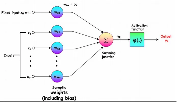
Figure 1 shows a typical neuron model, which is comprised of two parts. The first part is 285
the accretion of signals, where the input signals (input data) are gathered for a sum. As shown in 286
the following equation (eq.5), each weight (wi) equals a data dimension (xi), while (w0) as a bias is 287
correspondent to the intercept or constant term of the function. While the constant is set to ‘‘1'' as 288
the input of 0th dimension, the bias is managed as the weight of 0th dimension. This is also called 289
affine transformation (Lee, Chen, Yu, & Lai, 2018). 290
𝑍 = 𝑏𝑖𝑎𝑠 + ∑𝑚𝑖=1𝑋𝑖𝑊𝑖 = ∑𝑚𝑖=0𝑋𝑖𝑊𝑖 (5) 291
292
Figure 1.Typical neural network
The second part is the initiation of the function, where the obtained activation value is used 294
for the nonlinear compressed transformation to extricate a nonlinear eigenvalue. The frequently-295
used activation functions include ReLU, Sigmoid, and Tanh (Lee, Chen, Yu, & Lai, 2018). A 296
neural network is a network based on the interconnection between artificial neurons. The 297
feedforward neural network (FNN) or multilayer perceptron (MLP) is a neural network that 298
permits the feedforward connection of neurons. The input of data is known as the input layer, while 299
the output of results is termed as the output layer; the layers between the input layer and the output 300
layer are called the hidden layers (Lee, Chen, Yu, & Lai, 2018). MLP is a supervised algorithm 301
that learns a function 𝑓(. ): 𝑅𝑚 → 𝑅𝑜 by training on a given dataset, where 𝑚 is the dimension for 302
input and 𝑂 is the output dimension. Provided a set of features 𝑋 = 𝑥1, 𝑥2, 𝑥3, … , 𝑥𝑚 and target 𝑦, 303
it can learn a non-linear function for either classification or regression. 304
305
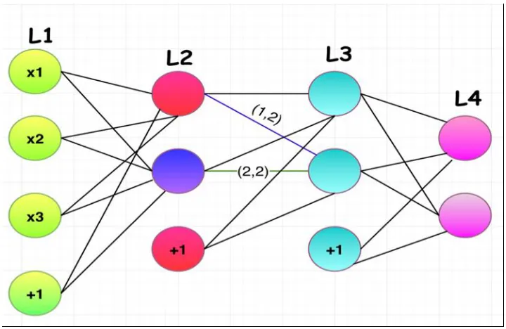
Figure 2.Feed-forward neural network
Figure 2 shows a 4 layered neural network, where the first layer (L1) is the input layer; L2 307
and L3 are the hidden layers; L4 is the output layer; 𝑎𝑖,𝑗(𝑙) refers to the connection weight of “i” 308
(ordinal number) neuron on layer I and “j” (ordinal number) neural on layer I+1; 𝑎𝑗𝑙 denotes the 309
connection between the bias on layer I and “j” neuron on layer I+1; and 𝑎𝑗𝑙 implies the activation 310
value (output value) of the “I” neuron on layer I, and the activation value of the blue neuron in the 311
picture is 𝑎2(2) (Lee, Chen, Yu, & Lai, 2018). 312
Voted Perceptron (VP)
313
It is designed for linear classification, that combines the Rosenblatt's perception algorithm 314
with Helmbold and Warmuth's leave-out method. All weight vectors confronted during the 315
learning process vote on a prediction. The measure of the accuracy of a weight vector, based on 316
the number of trials in which it correctly classifies instances, is used as the number of votes given 317
to the weight vector. The output a voted perceptron is given by (eq.6) when given labeled data is 318
(𝑥𝑖, 𝑦𝑖) where 𝑦 is +1 or -1 (mesothelioma or healthy):
319
𝑦𝑖 = 𝑠𝑖𝑔𝑛 {∑ 𝑐𝑝 𝑠𝑖𝑔𝑛(𝑤𝑝, 𝑥)
𝑃
𝑝=0
} (6) 320
Where 𝑥 are inputs, 𝑝 = 0,1,2, … , 𝑃;𝑤𝑝 are weights, 𝑦𝑖 is the predicted class, and 𝑐𝑝is 321
the survival time (reliability of 𝑤𝑝). 322
Hoeffding Tree
It is also known as Very Fast Decision Tree (VFDT) is a tree algorithm for data stream 324
classification. The Hoeffding tree is an incremental decision tree learner for a large dataset, that 325
assumes that the data distribution is constant over time. It grows a decision tree based on the 326
theoretical guarantees of the Hoeffding bound. In other words, VFDT employs Hoeffding bound 327
to decide the minimum number of arriving instances to achieve a certain level of confidence in 328
splitting the node. The confidence level determines the proximity of the statistics between the 329
attribute chosen by VFDT and the attribute chosen by decision tree for batch learning. 330
Clojure Classifier (CC)
331
It is a wrapper classifier developed in Clojure programming language. It mandates to have 332
at least a learn-classifier function and distribution-for-instance function. The learn-classifier 333
function takes an object and a string (nullable) and returns the learned model as a serializable data 334
structure. The distribution-for-instance function takes an instance to be predicted and a model as 335
an argument and returns the prediction as an array. 336
2.1.1. Primal Estimated sub-Gradient Solver for SVM 337
It is also known as s-Pegasos. It performs SGD on a primal objective (eq. 7,8) with 338
carefully chosen step size. 339
𝜆 2
𝑤
𝑚𝑖𝑛 ||𝑊||2+ 1
𝑚 ∑ 𝑙(𝑊; (𝑋, 𝑦)) (7)
(𝑥,𝑦)∈𝑆
340
Where 341
3.2.Model evaluation
343
While evaluating supervised machine learning models, it is important to measure each model’s 344
classification accuracy, f-measure, recall, precision, root mean squared error (RMSE), receiver
345
operating characteristic (ROC), and precision-recall curve (PRC). 346
Classification accuracy is the metric for evaluating classification models. It is the fraction of 347
predictions or classification that a model performs correctly. Classification accuracy can be 348
calculated by the given equation (eq.9) 349
𝐴𝑐𝑐𝑢𝑟𝑎𝑐𝑦 = 𝑁𝑢𝑚𝑏𝑒𝑟 𝑜𝑓 𝑐𝑜𝑟𝑟𝑒𝑐𝑡 𝑝𝑟𝑒𝑑𝑖𝑐𝑡𝑖𝑜𝑛 𝑇𝑜𝑡𝑎𝑙 𝑛𝑢𝑚𝑏𝑒𝑟 𝑜𝑓 𝑝𝑟𝑒𝑑𝑖𝑐𝑡𝑖𝑜𝑛 =
𝑇𝑃 + 𝑇𝑁
𝑇𝑃 + 𝑇𝑁 + 𝐹𝑃 + 𝐹𝑁 (9) 350
Where TP = Ture positive; TN = True negative; FP = False positive; FN = False negative. 351
The ROC curve is the graphical representation of the true positive rate (TPR) against the 352
false positive rate (FPR) at different threshold settings. In the machine learning domain, a TPR is 353
also known as sensitivity, recall or "probability of detection." Similarly, an FPR is known as the 354
fall-out or "probability of false alarm” and can be calculated as (eq. 10). The ROC curve is thus 355
the sensitivity as a function of fall-out. 356
𝐹𝑃𝑅 = (1 − 𝑠𝑝𝑒𝑐𝑖𝑓𝑖𝑐𝑖𝑡𝑦) (10) 357
Regarding information retrieval undertakings with binary classification (relevant or not 358
relevant), precisionis the segment of retrieved instances that are relevant, whereas recall, also 359
known as sensitivity is the fraction of retrieved instances to all relevant instances. In this context 360
(x-axis) and precision (y-axis), where recall and precision are determined using the given formula 362
(eq. 11,12) respectively. 363
𝑅𝑒𝑐𝑎𝑙𝑙 = 𝑇𝑃
(𝑇𝑃 + 𝐹𝑁) (11) 364
𝑃𝑟𝑒𝑐𝑖𝑠𝑖𝑜𝑛 = 𝑇𝑃
(𝑇𝑃 + 𝐹𝑃) (12) 365
f-measure, also known as F1-score is the harmonic mean of precision and recall (eq.13), where
f-366
measure reaches its best at 1 and worst at 0. 367
𝑓1 𝑠𝑐𝑜𝑟𝑒 = 2 ∗ (𝑝𝑟𝑒𝑐𝑖𝑠𝑖𝑜𝑛 ∗ 𝑟𝑒𝑐𝑎𝑙𝑙)
𝑝𝑟𝑒𝑐𝑖𝑠𝑖𝑜𝑛 + 𝑟𝑒𝑐𝑎𝑙𝑙 (13) 368
The root-mean-square error (RMSE) is a measure of performance of a model. It does this 369
by computing the difference between predicted and the actual values as given below (eq. 14). 370
𝑅𝑀𝑆𝐸 = √∑(𝑥𝑖 − 𝑦𝑖)
2
𝑁
𝑁
𝑖=1
(14) 371
Where (𝑥𝑖 − 𝑦𝑖) is the difference between predicted and actual value and N is the sample size. 372
4. Results
373
Phase 1
374
As shown in table 2, SGD, AdaBoost.M1, KLR, MLP, VFDT generates perfect results with 375
100% accuracy, precision, recall, and f-measure. These algorithms also return the highest possible 376
In this phase, the high accuracy of 100% indicates that results obtained from biopsy and 378
imaging tests are very strong predictors of MM. This result validates the significance of biopsy 379
and imaging results ("diagnosis method") from a data science viewpoint. 380
Table 2. Comparing classification accuracy (phase-1) 381
Algorithm SGD AdaBoost.M1 KLR MLP VP VFDT CC s-Pegasos
Classification
accuracy (%)
100 100 100 100 70.38 100 70.38 99.36
f-measure 1.00 1.00 1.00 1.00 0.83 1.00 0.83 1.00
Recall 1.00 1.00 1.00 1.00 1.00 1.00 1.00 1.00
Precision 1.00 1.00 1.00 1.00 0.70 1.00 0.70 0.99
ROC 1.00 1.00 1.00 1.00 0.50 1.00 0.50 0.99
PRC 1.00 1.00 1.00 1.00 0.70 1.00 0.70 0.99
RMSE 0.00 0.00 0.00 0.00 0.54 0.01 0.54 0.04
382
Phase 2 demonstrates the relevance of pre-diagnosis data. It also shows the behavior of all 383
predicting models post removal of “diagnosis method” and other post-diagnosis data. 384
Phase 2
385
Boruta algorithm confirmed five relevant attributes that are enough to predict the presence 386
of Mesothelioma without any loss in model's performance. In other words, the selected attributes 387
alone can prognosticate MM with the same accuracy as all other pre-diagnosis predictors when 388
taken together as input. The relevant predictor identified were c-reactive protein, platelet count,
389
duration of symptoms, gender, and pleural protein. 390
This method neither downgrades the remaining predictors nor does it recommend revising 391
the regular clinical procedures. Figure 3 below shows the attributes recognized by Boruta 392
candidate explanatory variables. The green box plots refer to the relevant attributes whereas the 394
red ones are identified as unimportant (from a data science viewpoint). The blue boxplots 395
correspond to minimal, average and maximum Z score of a shadow attribute created by the Boruta 396
algorithm. The following table 3 compares the different performance measures of each algorithm 397
used in this study. 398
399
Figure 3.Boruta plot for feature selection
400
AdaBoost outperformed all other models with the highest classification accuracy of 401
71.29%. Excluding “diagnosis method” from the prediction model resulted in decreased accuracy. 402
However, this phase has its own advantage. Despite lower accuracy, phase-2 helps reducing 403
diagnostic expenses. 404
Table 3. Comparing classification accuracy (phase-2) 405
Algorithm SGD AdaBoost.M1 KLR MLP-C VP VFDT CC s-Pegasos
Classification
accuracy (%)
69.23 71.29 69.51 64.11 70.38 70.38 70.38 67.03
Recall 0.80 0.86 0.93 0.84 1.00 1.00 1.00 0.81
Precision 0.74 0.74 0.76 0.75 0.70 0.70 0.70 0.75
ROC 0.58 0.61 0.65 0.61 0.50 0.50 0.50 0.58
PRC 0.74 0.77 0.82 0.79 0.70 0.70 0.70 0.74
RMSE 0.55 0.45 0.46 0.57 0.54 0.46 0.54 0.57
406
Discussion
407
An accurate diagnosis of MM is crucial at both the individual and public health level. It 408
has necessary medicolegal significance due to diagnosis‐related compensation (Ascoli, 2015). 409
However, prognosticating MM is challenging due to its composite epithelial pattern and low 410
likelihood of occurrence (Ascoli, 2015). To advocate the prognosis of MM with high accuracy and 411
low diagnostic cost, the current study designed and implemented a prediction model comprising 412
of two phases. (phase 1 and 2). 413
To our knowledge no previous studies have implemented our AI models and focused on 414
reducing diagnosis expenses by eliminating biopsy and imaging test results from the dataset. 415
Phase-2 of our study proposes AdaBoost.M1 algorithm that can identify high risk patients at lower-416
cost by taking only blood test results and patient’s demographic data. Outcome from phase-2 can 417
provide the doctors with a list of high-risk patients. Doctors and other healthcare providers can 418
then prescribe biopsy tests only to the identified patients for reconfirming MM using phase-1 419
model with optimal accuracy. This approach will reduce unnecessary biopsy tests and thus reduce 420
overall expenses by up to $7900 (Molinari, 2018). 421
The recommended model (AdaBoost) in phase-2 requires c-reactive protein, platelet count,
422
duration of symptoms, gender, and pleural protein as its input. The expenses to collect the required 423
input data can range from. $100 to $200 (Practo, 2017) for Protein Total Pleural Fluid (pleural
protein), $40 to $70 (Haiken, 2011) for c-reactive protein test, and $6 to $167 (Pinder, 2012) for 425
complete blood count (platelet count) depending up on the location. These factors can also 426
advocate early prognosis of MM; Moreover, studies have shown that higher (>1 mg/dL) c-reactive 427
protein influences mesothelioma (Takamori, et al., 2018) (Ghanim, et al., 2012), another study at 428
the University of Maryland determined the clinical significance of preoperative thrombocytosis 429
(high count of platelets), in patients with MPM (Li, et al., 2017). 430
5. Conclusion
431
Our study identifies that the diagnosis method (biopsy and imaging test results), c-reactive protein,
432
platelet count, duration of symptoms, gender, and pleural protein plays a significant role in 433
diagnosing MM. However, effective diagnosis methods such as pleuroscopy (lungs) or 434
laparoscopy (abdomen), thoracotomy (lungs) or laparotomy (abdomen), and imaging tests (CT 435
scan and MRI) are expensive. This study proposes two approaches to predict MM, each having its 436
advantages and limitations. The first approach (phase-1) uses all predictors from mesothelioma 437
data and produces 100% classification accuracy. The second approach (phase-2) ensures cost 438
reduction. Our study recommends AdaBoost algorithms for MM prognosis and suggests using 439
pase-2 approach to short list high risk patients followed by phase 1 to confirm MM. 440
441
442
443
444
445
446
448
449
450
451
452
453
List of abbreviations
454
MPM – Malignant Pleural Mesothelioma 455
MM – Malignant Mesothelioma 456
PM – Pleural Mesothelioma 457
ROC – Receiver Operating Characteristics 458
PRC – Precision-recall curve 459
DT – Decision tree 460
VFDT – Very fast decision tree 461
MLP – Multi-layer perceptron 462
SGD – Stochastic gradient descent 463
KLR – Kernel logistic regression 464
AdaBoost – Adaptive boosting 465
RMSE – Root mean squared error 466
ANN – Artificial neural network 467
SVM – Support vector machine 468
S-Pegasos - Primal Estimated sub-Gradient Solver for SVM 469
VP – Voted perceptron 471
TP – Ture positive 472
TN – True negative 473
FP – False positive 474
FN – False negative 475
TPR – Ture positive rate 476
FPR – False positive rate 477
WBC – White blood cell 478
HGB – Hemoglobin 479
PLT – Platelet count 480
LDH – Blood lactic dehydrogenize 481
ALP – Alkaline phosphate 482
CRP – C reactive protein 483
AUC – Area under the curve 484
Declarations
485
- Ethics approval and consent to participate - All data were collected with the permission of the 486
organization and the study ensure no leakage of any patient’s medical and personal 487
information. 488
- Consent for publication - Not applicable 489
- Availability of data and material - All data analyzed during this study are included in this 490
published article and its supplementary information files. 491
- Competing interests - The authors declare that they have no competing interests 492
- Authors’ contribution - AC analyzed, interpreted the mesothelioma data. AC performed the 494
time series forecasting and evaluated the model. 495
- Acknowledgments - Not applicable 496
-497
Reference
498
Ascoli, V. (2015). Pathologic diagnosis of malignant mesothelioma: Chronological prospect and 499
advent of recommendations and guidelines. Ann Ist Super Sanità, 51(1), 52-59. 500
Bueno, R., Stawiski, E., Goldstein, L., & al., e. (2016;). Comprehensive genomic analysis of 501
malignant pleural mesothelioma identifies recurrent mutations, gene fusions and splicing 502
alterations. Nat Genet, 48, 407–416. 503
Choudhury , A. (2018). Identification of Cancer: Mesothelioma's Disease Using Logistic 504
Regression and Association Rule. American Journal of Engineering and Applied Sciences,
505
11(4), 1310-1319. 506
Choudhury, A., & Greene, C. (2018). Evaluating Patient Readmission Risk: A Predictive Analytics 507
Approach. American Journal of Engineering and Applied Sciences, 11(4), 1320-1331. 508
Frauenfelder, T., Tutic, M., Weder, W., & al., e. (2011;). Volumetry: an alternative to assess 509
therapy response for malignant pleural mesothelioma? Eur Respir J ., 38, 162-168. 510
Friedin, R. B. (2012, May 11). Am I going to die because I cannot afford the test? (KevinMD) 511
Retrieved December 26, 2018, from https://www.kevinmd.com/blog/2012/05/die-afford-512
test.html 513
Ghanim, B., Hoda, M. A., Winter, M.-P., Klikovits, T., Alimohammadi, A., Hegedus, B., . . . 514
multimodality treatment including radical surgery in malignant pleural mesothelioma: a 516
retrospective multicenter analysis. . Annals of Surgery, 256(2), 357–362. 517
Gill, R., Naidich, D., Mitchell, A., & al., e. (2016;). North American multicenter volumetric CT 518
study for clinical staging of malignant pleural 30. mesothelioma: feasibility and logistics 519
of setting up a quantitative imaging study. . J Thorac Oncol , 11, 1335–1344. 520
Haiken, M. (2011, July 17). 3 New Medical Tests that Can Save Your Life - But You Have to Ask. 521
(Forbes) Retrieved December 26, 2018, from
522
https://www.forbes.com/sites/melaniehaiken/2011/06/17/3-lifesaving-new-medical-tests-523
you-have-to-ask-for/#2df47f75398a 524
Ilhan, H. O., & Celik, E. (2016). The mesothelioma disease diagnosis with artificial intelligence 525
methods. 2016 IEEE 10th International Conference on Application of Information and
526
Communication Technologies. Baku. 527
James, G., Witten, D., Hastie, T., & Tibshirani, R. (2017). An Introduction to Statistical Learning:
528
with Applications in R. New Yrok: Springer. 529
Kuhn, M., & Johnson, K. (2018). Applied Predictive Modeling. New York: Springer. 530
Lee, S.-J., Chen, T., Yu, L., & Lai, C.-H. (2018). Image Classification Based on the Boost 531
Convolutional Neural Network. IEEE Access, 6, 12755-12768. 532
Leigh, J., Corvalan, C., Grimwood, A., Berry, G., Ferguson, D., & al., e. (1991;). The incidence 533
of malignant mesothelioma in Australia 1982–1988. Am J Ind Med , 20, 643–655. 534
Li, Y. C., Khashab, T., Terhune, J., Eckert, R. L., Hanna, N., Burke, A., & Alexander, H. R. (2017). 535
Preoperative Thrombocytosis Predicts Shortened Survival in Patients with Malignant 536
Peritoneal Mesothelioma Undergoing Operative Cytoreduction and Hyperthermic 537
Liaw, A., & Wiener, M. (2002). Classification and Regression by random Forest. R News, 2(3), 539
18-22. 540
Lotfi, E., & Keshavarz, A. (2014). Gene expression microarray classification using PCA-BEL. 541
Computers in Biology and Medicine,, 54, 180-187. 542
McDonald, C., J., & McDonald., A. D. (1996). The epidemiology of mesothelioma in historical 543
context. . European Respiratory Journal , 9, 1932-1942. 544
Mesothelioma News. (2018, July 28). What Mesothelioma Does to the Body. Retrieved August 25, 545
2018, from http://www.mesotheliomanews.com/medical/mesothelioma-diagnosis/pleural-546
mesothelioma/ 547
Metintas, M., Metintas, S., Guntulu AK, S. E., Alatas, F., Kurt, E., Uugun, I., & Yildirim, H. 548
(2008). Epidemiology of pleural mesothelioma in a population with non-occupational 549
asbestos exposure. Respirology, 13, 117-121. 550
Miron, B. K., & Witold, R. R. (2010). Feature Selection with the Boruta Package. Journal of
551
Statistical Software, 36(11), 2-13. 552
Molinari, L. (2018, November Thursday ). Mesothelioma Treatment Costs. (Cancer Alliance ) 553
Retrieved December Saturday, 2018, from
554
https://www.mesothelioma.com/treatment/mesothelioma-treatment-costs/ 555
Nilsson, R., Peña, J. M., Björkegren, J., & Tegńer, J. (2007). Consistent Feature Selection for 556
Pattern Recognition in Polynomial Time. The Journal of Machine Learning Research, 8, 557
612. 558
Pass, H., Giroux, D., Kennedy, C., & al., e. (2016). The IASLC mesothelioma staging project: 559
improving staging of a rare disease through 29. international participation. J Thorac Oncol,
560
Paydar, K., R, S., Kalhori, N., Akbarian, M., & Sheikhtaheri, A. ( 2017). A clinical decision 562
support system for prediction of pregnancy outcome in pregnant women with systemic 563
lupus erythematosus. International Journal of Medical Informatics , 97, 239-246. 564
Peto, J., Hodgson, J., Matthews, K., & Jones, J. (1995;). Continuing increase in mesothelioma 565
mortality in Britain. Lancet, 345, 535–539. 566
Pinder, J. (2012, December 27). How much does a blood test cost? It could be $6, or $167 . (Clear 567
Health Cost Beta) Retrieved December 26, 2018, from
568
https://clearhealthcosts.com/blog/2012/12/how-much-does-a-blood-test-cost-it-could-be-569
16-or-117/ 570
Pope, T. P. (2010, February 4). When Patients Can’t Afford Their Care. (New York Times) 571
Retrieved December 26, 2018, from https://well.blogs.nytimes.com/2010/02/04/when-572
patients-cant-afford-their-care/ 573
Practo. (2017, December 11). Protein Total Pleural Fluid. Retrieved December 25, 2018, from 574
https://www.practo.com/tests/protein-total-pleural-fluid/p 575
Ron, K., & George, H. J. (1997). Wrappers for feature subset selection. Artificial Intelligence, 97, 576
273-324. 577
Selby, K. (2018, December 20). Mesothelioma Diagnosis . (Asbestos.com and The Mesothelioma 578
Center) Retrieved December 22, 2018, from
579
https://www.asbestos.com/mesothelioma/diagnosis/ 580
Silvester, J. (2016, September 27). Most of the World Doesn't Have Access to X-Rays. (Health) 581
Retrieved December 26, 2018, from
582
Spirtas, R., Beebe, G., Connelly, R., Wright, W., Peters, J., & al., e. (1986;). Recent trends in 584
mesothelioma incidence in the United States. Am J Ind Med, 9, 397-407. 585
Stefano, P., Rosa, F., & Paola, M. e. (2015). Differential diagnosis of pleural mesothelioma using 586
Logic Learning Machine. BMC Bioinformatics , 16, 1471-2105. 587
Takamori, S., Toyokawa, G., Shimokawa, M., Kinoshita, F., Kozuma, Y., Matsubara, T., . . . et.al. 588
(2018). The C-Reactive Protein/Albumin Ratio is a Novel Significant Prognostic Factor in 589
Patients with Malignant Pleural Mesothelioma: A Retrospective Multi-institutional Study 590
. Ann Surg Oncol, 25(17), 1-8. 591
Tin, K. (1995). Random decision forests. Proceedings of 3rd International Conference on
592
Document Analysis and Recognition. Montreal. 593
Vogelzang, N., Rusthoven, J., Symanowski, J., & al., e. (2003). Phase III study of pemetrexed in 594
combination with cisplatin versus cisplatin alone in patients with malignant pleural 595
mesothelioma. J Clin Oncol 2003; 21:2636–44., 21, 2636-2644. 596
Zalcman, G., Mazieres, J., Margery, J., Greillier, L., Audigier-Valette, C., Moro-Sibilot, D., . . . 597
et.al. (2016). Bevacizumab for newly diagnosed pleural mesothelioma in the Mesothelioma 598
Avastin Cisplatin Pemetrexed Study (MAPS): a randomised, controlled, open-label, phase 599
3 trial. Lancet, 387, 1405-1414. 600
601
602
List of figure legends
603
Figure 4: Typical neural network 604
Figure 2: Feed-forward neural network 605