PERFORMANCE COMPARISON BETWEEN KNN AND NSGA-II ALGORITHMS AS CALIBRATION APPROACHES FOR BUILDING SIMULATION MODELS

PERFORMANCE COMPARISON BETWEEN KNN AND NSGA-II ALGORITHMS

AS CALIBRATION APPROACHES FOR BUILDING SIMULATION MODELS

Shadi Basurra

1

and Ljubomir Jankovic

2 1

_{School of Computing and Digital Technology,}

2

_{Director, Zero Carbon Lab, Birmingham School of Architecture,}

Birmingham City University,

Birmingham, UK

[email protected]; [email protected]

ABSTRACT

In this paper, a study of calibration methods for a thermal performance model of a building is presented. Two calibration approaches are evaluated and compared in terms of accuracy and computation

speed. These approaches are the 𝑘 Nearest Neighbour

(KNN) algorithm and NSGA-II algorithm.

The comparison of these two approaches was based on the simulation model of the Birmingham Zero Carbon House, which has been under continuous monitoring over the past five years. Data from architectural drawings and site measurements were used to build the geometry of the house. All building systems, fabric, lighting and equipment were specified to closely correspond to the actual house. The preliminary results suggest that the predictive performance of simulation models can be calibrated quickly and accurately using the monitored performance data of the real building. Automating such process increases its efficiency and consistency of the results while reducing the time and effort required for calibration. The results show that both NSGA-II and KNN provide similar degree of accuracy in terms of the results closeness to measured data, but whilst the former outperforms the latter in terms of computational speed, the latter outperforms the former in terms of results wide coverage of solutions around the reference point, which is essential for calibration.

INTRODUCTION

There has been a growing industrial and academic interest in using optimisation tools to simulate existing buildings in order to optimise their real performance and reduce their energy consumptions through retrofitting. However, one main issue that is always observed is the performance gap which is the performance difference between the real building and the simulation model. Hence, model calibration is needed in this kind of scenarios. Model calibration is used to ensure that building thermal performance is represented accurately, in relation to architecture properties, mechanical systems, internal gains and building fabrics. During the calibration process, the input values of the model parameters are varied and tested, until the simulation model matches the monitored performance of the existing building.

Related work

Using building simulation is somewhat easier for new built projects, were building properties and parameters are given using the engineering design specification. However, designing a model to represent an actual building is not trivial, since it is difficult to know how the building’s internal/external components operate, and whether or not the technology or/and the building materials used have the same efficiency and properties, as they were when the building was built.

There are various advantages of using calibration in construction industry, some of which were listed by Claridge (2011), for example, in order to increase the building energy efficiency through a mix of technologies with reasonable cost and short payback time frame. Building simulation tools have been used to explore possible alternatives to achieve better energy performance with a shorter payback period. However, allocation of risks requires uncertainty quantification of projected cost effectiveness of technology options for a given retrofit project. Hence, using calibration to reduce this risk while reducing the performance gap encourages building owners to invest in retrofit with high confidence. Moreover, calibration can be used in commissioning activities of existing buildings, and for detecting faults in building performance.

experimental evidence; 2- hidden assumptions performed by various software implementations; 3- Energy models can be complex with many interactions; 4- uncertainties with basic properties of existing building.

Even for an experienced modeller, the trial-error approaches could be labour intensive and time consuming. They mostly depends on user experience and assumptions (Paul et al., 2011), hence, user’s skills and knowledge are critical for performing calibration, and have direct influence on the building model accuracy and calibration time span.

However, other methods beyond the trial-error approach have started to develop. The use of automated methods can help non-expert users when performing calibration process, hence, preventing manual tuning for each parameters, when dealing with numerous simulation runs and the lengthy calibration time required for traditional trial and errors methods. For example, the study by Tahmasebi and Mahdavi, (2012) and Monetti et al. (2015) use automated methods to fine-tune the model, which ensure the efficacy and consistency of the process and generated results.

This paper focuses on the computational aspect of two automated model-assisted calibration methods in terms of the proximity of results to the actual measured values, solution coverage and computation speed. These approaches are the k Nearest Neighbour (KNN) algorithm and the NSGA-II algorithm. A direct extension for this work would be to validate the calibrated models resulted from both algorithms with measured data and weather data from different years. However, this will also require conducting multiple detailed surveys to investigate how tenants behaviour changes overtime, and to look at other factors of performance degradation such as structural material defects/cracks etc.

The Birmingham Zero Carbon House is used as experimental evidence base for this investigation. It is a retrofitted Victorian house that has achieved a carbon negative performance, and it has been under detailed instrumental monitoring over the past five years. The data collected from the monitoring are utilised in the calibration process.

METHODOLOGY

𝑘-nearest neighbours’ algorithm (KNN) (Alt, 2001)

is a widely used technique for clustering and classification of data in data mining, and pattern recognition. It is a basic approach to find the most

similar 𝑘 number of points as nearest neighbour to a

given reference point on a solution space. In this study, we use the method proposed by Basurra et al. (2015) which uses KNN with density avoidance method to solve the problem of simulation model calibration. Inspite of their simplicity, KNN methods are among the best performers in a large number of classification problems. This is because KNN is

non-parametric which means the algorithm works without presumption of the primary data distribution. Thus, the algorithm requires no training phase before being used on a solution space. This is essential for calibration of simulation models since the real monitored data do not usually obey the typical theoretical assumptions made in the simulation model. Moreover, the algorithm is fast to perform, despite the fact that KNN bases its decision after calculating the entire solution space.

KNN is used for classification and regression. Classification is performed using the instance-based classifier by locating the nearest neighbour in the instance space and labelling the unknown instance with the same class label as that of the located

classified (known) neighbour. One of the

classification rules for KNN is to find the nearest neighbour using the inverse distance and majority

voting, which allows those neighbours where 𝑘 > 1 to

decide the outcome of the class labelling.

The process starts by measuring distances between the query points to the rest of the solution points. One of the most popular choices to measure the distances

is to use the Euclidean function. Given 𝑥 =

(𝑥1 , … , 𝑥𝑛 ) and 𝑦 = (𝑦1 , … , 𝑦𝑛 ), the distance is calculated as

𝑑𝐸(𝑥, 𝑦) = √∑𝑁𝑛=1(𝑥𝑛− 𝑦𝑛)2. (1)

KNN Regression is related to predict the outcome of a dependant variable given a set of independent variables. This is useful since it enables the prediction of the regions in which future candidate solutions will be populated.

The algorithm function

𝑘 is the number of nearest neighbours in the solution

space 𝑆: = (𝑝1, . . . , 𝑝𝑛) where 𝑝𝑛 is the solution

sample in the form 𝑝₁= (𝑥_𝑖, 𝑐_𝑖), where 𝑥_𝑖 solution

entry with all parameter values of the point 𝑝𝑖. 𝑐𝑖 is

the class that 𝑝𝑖 belongs to (see Figure 1).

 Start:

 For each 𝒑′_{= (𝒙}′_{, 𝒄}′₎  Calculate the distanced

𝒅(𝒙′, 𝒙𝒊) between𝒑′ and all 𝒑𝒊belonging to 𝑺  Re-organise all 𝒑𝒊 in accordance to their

distance

 Select the first 𝒌 points from the sorted list, those are the 𝒌 closest training samples to 𝒑′

 Allocate a class to 𝒑′ based on majority vote: 𝒄′ = 𝒂𝒓𝒈𝒎𝒂𝒙𝒚∑(𝒙𝒊, 𝒄𝒊) belonging to 𝑺, 𝑰(𝒚 = 𝒄𝒊). For 𝒑𝒊, where 𝒊 1,2, .. number of pints in𝒄𝒊

 End:

Figure 1: KNN algorithm steps

The selection of 𝑘 is critical. This is because a small

value of 𝑘 means that the results will be increasingly

make it computationally expensive, but also defeats the concept behind the KNN that solution ‘points’

that are near are likely to have similar

densities/classes. One simple approach suggested by

Richard et al. (2000) is to set 𝑘 as 𝑘 = √𝑛 where 𝑛

is the total number of points in the solution space. Density estimation for KNN

As discussed above, KNN ideally identify neighbour solutions scattered evenly in the solution space while covering various regions on the graph. However, if the reference point is adjacent to highly densely populated area of solutions, the algorithm only selects the solutions from the dense area, especially if the number of nodes located in that area exceeds the

calculated 𝑘 neighbours. This will worsen if all

detected nearest neighbours exist on the same location on the graph, as this would mean all design solutions are the same.

Various extensions have been performed to the KNN algorithm to consider density. Although classification is the primary application of KNN, density estimation can also be used in KNN. Density

estimation is a non-parametric method for

constructing a density estimate of results. This is very similar to Parzen-window which is essentially a data-interpolation technique (Richard et al, 2000).

For example, to estimate density at a point x, by

placing a circle centered at x and keep increasing its

size until k neighbours are captured. The density

estimation uses the following formulae:

𝑝(𝑥) = 𝑘/𝑛

𝑎 (2)

In the formula above, n is the total number of design

solutions, and a is the area of the circle. The

numerator is a constant and the density is influenced by its value. For example, the distance to the k nearest neighbour can also be seen as a local density estimate, and thus is used to detect outlier neighbours in the dataset. The larger the distance to the kNN, the lower the local density, the more likely the query point is an outlier and vice versa.

We use similar technique to KNN, but differ in the sense that instead of using density for anomaly detection, we use density calculation to select a fewer neighbours located in high dense areas. That is, the algorithm selects fewer solutions in local densely areas in order to cover wide range of areas in the solution space as long as they are located within reasonable distance from the reference point.

Density avoidance for KNN

Basurra et al., (2015) proposed a density avoidance algorithm which has been tested against various cases for this purpose. Our proposed density avoidance algorithm is briefly explained below.

Starting from a close by solution from the reference point, each solution will form a circular region with a constant radius R to capture all surrounding nodes in the solution space. For example, let us consider a

solution X of N solutions in the graph. X will perform

the density estimation and calculate the density using Equation (2).

If density is above a threshold, the node closest to X

(not the reference point), will be tagged as high-density node (HD). The whole process repeats again,

and X becomes the second closest node to the

reference point. In subsequent iterations, HD nodes are not selected to perform the density calculation, and will not be considered in the density check if they fall within the range within a circle area of another valid low-density node. Following these rules, all nodes in the solution space will be tagged as either HD or none.

Then we implement the KNN algorithm that selects

the closest 𝑘 neighbours, but also selects only those

which are not HD solutions. This was successfully implemented, and is shown in Figure 2.

 PROGRAM DensityExclusionAlgorithm:

 Using KNN, CALCULATE distances to all 𝑁solutions from Reference Point.

 Store the 𝑵 neighbours with their distances in a list 𝑳

 Sort list 𝑳 in a ascendant order putting least distant solutions at the top of 𝑳.

 LOOP through 𝑳 starting from the top, and select 𝑿 solution

 𝑿 Identify nearby neighbours from 𝑁 using a predefined radius

𝑹, and store them in a new list 𝑳2.

 𝑿 calculates density 𝑳2

 If (𝐷𝑒𝑛𝑠𝑖𝑡𝑦 > 𝑇ℎ𝑟𝑒𝑠ℎ𝑜𝑙𝑑 && 𝑁 ≠ 𝐻𝐷)

 THEN from 𝑳2, set “HD” to Neighbour closest to X

 ELSE DO NOTHING;  ENDLOOP

 CALCULATE neighbours of Reference Point with K number of neighbours.

 End

Figure 2 Pseudocode describing the steps of the density avoidance algorithm.

NSGA-II

Optimisation refers to the selection process that looks for the best solution in relation to certain criteria, from a solution space that contains a set of available alternatives (George, 2014). It can be performed using single or multiple objectives. Single objective optimisation is the easiest as the algorithm looks for the best possible solution from the answer set, and this is known as the global optimum. Multi-objective optimisation is computationally more complex as the objectives normally have negative correlations, such as minimising the cost of retrofitting, while maximising the energy efficiency performance (Coello et al., 2006).

2013); and iterative, e.g. gradient-based, which can take many iterations to compute a local minimum by taking steps proportional to the negative of the gradient (Evins, 2013). For more details about the many optimisation approaches currently available, the reader is invited to consult technical literature, such as Coello (1999).

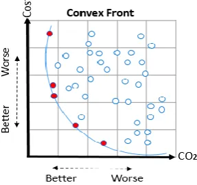
In reality, there are tens of optimisation methods, but only a few have been widely recognised and used. One of these is the Non-dominated Sorting Genetic Algorithm II (NSGA-II) (Deb et al., 2002), which has become very popular in the recent years due to its computational efficiency and good performance. Like most optimisation techniques, it searches through the solution space to find a set of optimal trade-offs, while treating all objectives as being equally important (i.e. non-dominated solutions) and the output set contains the optimal solutions, called Pareto fronts as can be seen from Figure 3.

Figure 3: Illustrates the convex Pareto fronts in red.

Crowding function

NSGA-II ranks Pareto optimum solutions based on their values, but also like KNN it uses density function to estimate density of dominant solutions around the optimum. This is performed by calculating the average distance to other points on either side of the solution. This density value is the so-called crowding distance, and is used to prioritise non-dominant solutions when they have similar ranks. In this case, NSGA-II chooses the solution that exists in the less dense area in the graph. Moreover, it does not require external memory and this makes it computationally efficient with large sets of solutions. We adjusted the optimisation function in JEPlus +EA (jeplus.org, 2016) to find optimal solutions that are closets to the reference point instead of the default optimisation objectives. In this scenario, the optimisation through NSGA-II, will search the solution space to find a set of optimal trade-offs while targeting the reference point.

PRE-CALIBRATION PROCEDURE

For the purpose of this research, we have selected the Birmingham Zero Carbon house (Christophers, 2014), which was originally built in 1840, and has

been retrofitted recently to achieve zero carbon performance. It has been selected based on availability of information for the energy model, good quality observations and easy access to the site for operational adjustments. Geometry of the model in DesignBuilder (Designbuilder.co.uk, 2016) is shown in Figure 4.

Figure 4 Birmingham Zero Carbon House model geometry - front and rear view

A comprehensive data monitoring system was installed in the house, which consists of internal temperature, relative humidity and energy flow sensors, as well as external air temperature sensor and a solar radiation instrument. Hence, accurate monitored data were collected and used for the calibration purpose discussed in this paper.

Actual weather data was collected from The Centre

for Environmental Data Archival (CEDA)

(ceda.ac.uk, 2016), which represent the closest viable data to zero carbon house site. This weather data file was modified, to include site-specific measurements obtained from the instrumentation system in the Zero Carbon House, and later was converted into '.epw' format used by EnergyPlus (Crawley, 2001). This process is described in detail by Jankovic (2012). We have run the optimisation with two objectives, actual discomfort hours and carbon emissions produced by the building.

We have calculated the first objective by generating temperature distribution scatter graphs showing the relative humidity and operative temperature intervals during the occupied period. Subsequently, we used

ANSI/ASHRAE Standard 55-2004 (ASHRAE,

2014), for thermal environmental conditions for human occupancy to calculate the total discomfort hours for one year.

Figure 5 Comfort hours (in black) and discomfort hours (in grey) derived using ASHRAE 55-2004.

RESULTS

Using the thermal comfort algorithm, we realised that the total number of comfort hours is 2128 in the year 2012. However, related occupant survey results confirm that occupants were close to thermal neutrality, despite the high number of discomfort hours calculated above. From our monitoring equipment, we also calculated CO2 produced by the building during the same year. The building achieved

carbon negative performance, with negative

emissions of -661.60 CO2 (kg) (Jankovic, 2012). We used these results to form a reference point in the solution space. KNN with the density avoidance algorithm use this reference point to identify the closest neighbours to the reference point, hence finding the closest design solutions between the measured and simulated results. However, NSGA-II target the generated reference point, forming Pareto solutions, to improve the correspondence between actual and monitored values towards a one-to-one line with an intercept of zero in the ideal case. For the purpose of comparison, we use the same simulation settings and optimisation duration when optimising the building model with both KNN and NSGA-II algorithms. With this knowledge, we can explore possible solutions - in the form of theoretical extensions or refinements to the input values of the model parameters.

Table 1 below shows the parameters used to calibrate the model. Most of these values were identified in Jankovic and Huws (2012) and Huws and Jankovic (2014) as sensitive inputs to cause significant influence in the model’s output. These input variables identified 70560 solution combinations for optimisation.

Table 1 Optimisation / parametric analysis settings used for the building model

Name Min

Value Max Value

Step

Mechanical ventilation (ach)

0.12 5 0.5

Natural ventilation 0 0.003 0.0005

rate (ach)

Domestic hot water setpoint temp (°C)

30 80 10

Equipment power density (W/m2)

1 6 1

Lighting density (W/m2)

2 5 0.5

Internal Wall Insulation

- - 2 Options of wall insulations

External wall Insulation

- - 2 Options of wall insulations

Optimisation was performed remotely using

JEPlus+EA via the ENSIMS X3200 Simulation Server located at Birmingham City University. This

allowed quick simulation and optimisation,

minimising the number of results in the solution space while finding a trade-off between the input design parameters according discomfort hours and CO2 emissions.

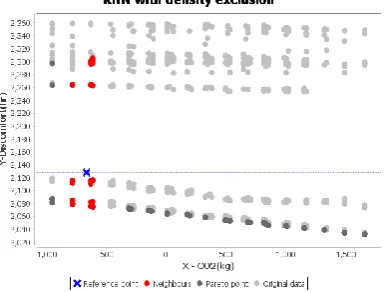
Figure 6 shows the results from the optimisation process using JEPlus+EA with KNN. The Figure also demonstrates the reference point as a blue diagonal cross in the solution space. The dark grey solutions represents the Pareto fronts from optimising the building model with various sets of parameter ranges. It also shows the neighbour solutions in red after being identified by the KNN with density avoidance algorithm. Figure 6 shows clearly that the total

number of points n in the solution space is 1306,

thus, using the square root as suggested by Richard et al. (2000), the total number of K neighbours becomes 36.14 which are shown in red in Figure 6.

KNN automatically identifies the closest solutions to the reference point, and reduces the results to 36.14, hence minimising the time needed to calibrate the results further toward the reference point. Due to the page limitation of the paper, Table 2 only shows a sample set of the best design solutions formed as red neighbour dots in Figure 7. The best calibrated model achieved using KNN is -627.6 CO2 (kg) and 2116 discomfort hours, hence, 0.5% error rate for CO2 (kg), and 0.6% error rate for discomfort hours in relation to the reference point.

To use NSGA-II for calibration, we had to alter the objective functions since the reference point in this study consist of only two parameter values CO2 and annual discomfort hours. This was performed through the following Equation 1 to calculate the objective function for carbon emission and discomfort hours.

𝑜𝑏𝑗 = 𝑎𝑏𝑠(𝛽 − 𝛼) (1)

Where obj is the objective value, 𝑎𝑏𝑠() is the

absolute value function. 𝛽 denotes to the monitored

value and 𝛼 represents the outcome of each

number of n solutions 1097, and 42 of which tagged as Pareto fronts and are depicted in red colour. These are effectively the calibrated solutions with the least performance gap as they are closest to their origin axis on a graph. The optimal calibrated model obtained using NSGA-II is -652.1 CO2(kg) and 2138 discomfort hours, hence, 1.4% uncertainty ratio for CO2 (kg), and 0.5% uncertainty ratio for discomfort hours in relation to the reference point .Table 3 shows a sample set of the Pareto fronts identified by NSGA-II.

Figure 6 KNN in operation while using the density avoidance algorithm

From Figures 6 and 7, it is clear that KNN and NSGA-II performed well to identify close solutions to the reference point. They both mange to reduce the number of calibrated results from approximately hundreds to an average of 40 solutions with the least possible performance gap.

Figure 7 NSGA-II in operation while using the built-in crowdbuilt-ing algorithm

DISCUSSION

In both cases, the optimisation process ran for the same 24 hours duration, which was the reason for both algorithms to be able to run a similar number jobs for this experiment. However, network throughput and server memory could also influence the speed of the algorithms.

An advantage of the NSGA-II is that the results generated at the end of the optimisation process are

the final solutions with the least possible

performance gap. However, KNN requires post processing when the optimisation is complete. Moreover, if further refinements are desired, more iterations are required to achieve closer relationship between the simulated and actual data

Figure 6 shows that KNN managed to identify neighbour solutions scattered around the reference point almost evenly in all directions in the solution space, and each discovered neighbour encapsulates

Table 2 Detailed parametric settings of the K neighbour solutions (displayed in Red in Figure 6)

Table 3 Detailed parametric settings of the Pareto fronts (displayed in Red in Figure 7)

M ec h an ic al v en ti la ti o n (a ch ) N at u ra l v en ti la ti o n ra te ( ac /h ) Ex te rn al w al l in su la ti o n Ex te rn al w al l in su la ti o n Li g h ti n g D en si ty (W /m2 ) Eq u ip me n t P o w er D en si ty (W /m2 ) D o mes ti c h o t w at er set p o in t te m p er at u re C O 2 ( k g ) D isco mf o rt (h r)

0.12 0 1 1 2 2 30 -627.581 2115.5

0.12 0 1 2 2 2 30 -627.581 2110.5

0.12 0.001666667 1 1 3 1 30 -609.474 2116

0.12 0.001111111 2 2 2.5 1 30 -777.712 2079.5

0.12 5.56E-04 2 2 2.5 1 30 -777.712 2079.5

0.12 0 2 2 2.5 1 30 -777.712 2079.5

0.12 0.002777778 2 2 2.5 1 30 -777.712 2079.5

0.62 0.001666667 1 1 3 1 30 -609.474 2300.5

1.62 0.002777778 2 1 3 1 30 -609.474 2297

3.12 0 2 2 3 1 30 -609.474 2305

M ec h an ic al v en ti la ti o n (a ch ) N at u ra l v en ti la ti o n ra te ( ac /h ) Ex te rn al w al l in su la ti o n Ex te rn al w al l in su la ti o n Li g h ti n g D en si ty (W /m2 ) Eq u ip me n t P o w er D en si ty (W /m2 ) D o mes ti c h o t w at er set p o in t te m p er at u re C O 2 ( k g ) D isco mf o rt (h r)

0.12 0.001111111 1 1 2 1 80 -652.1 2137.5

0.62 0.001111111 1 2 2 2 30 -493.1 2296.5

0.62 0.003333333 2 2 2 2 30 -525.6 2264

0.12 5.56E-04 1 1 2 2 30 -649.1 2140.5

all values for the parameters used during the simulation. This is useful for calibration since the aim is to capture all possible solution combinations, regardless of their design values, to minimise the performance gap with the actual building.

From these neighbour solutions, using minimum and maximum values; 1) we can break the range further into smaller steps to be used as input during subsequent simulation to bring the solutions closer to the reference point; 2) it will help when performing sensitivity analysis to identify the least sensitive parameter using maximum and minimum functions.

For example, Domestic hot water setpoint

temperature in Table 2 has the same output value 30 in all identified solutions. Since this has no effect on the output, fixing this parameter with the value 30 in subsequent calibration iteration is likely to bring the model closer to the reference point.

From Figure 7, it is apparent that NSG-II discovered the best solutions from the top right area from the reference point. Although, KNN identified far worst results in that region in the solution space in comparison to NSGA-II, it has discovered much closer solutions to the reference point in the bottom right and left regions from the reference point that were completely unavailable in NSGA-II results.

CONCLUSION

According to previous studies, calibration is still largely performed on the bases of trial-error approaches, which depend on user’s assumptions and experience. Even for an experienced modeller, trial-error approaches could be labour intensive and time consuming. Hence, the use of automated methods allows experts and non experts to perform calibration effectively without the manual tuning of each parameter, but also swiftly speeding the time required for calibration. Our aim of this paper was to compare the KNN and NSGA-II for calibration of building simulation, and evaluate both approaches in terms of speed, results quality and coverage.

The first approach was the nearly unbiased KNN algorithm that was used to identify the solutions with the lowest performance gap based on a set of reference points that corresponds to the actual building performance. Density avoidance algorithm was used to further refine the solutions by finding regions in the space of input factors for which the model output was either maximum or minimum to meet the optimum criterion, thus fine tuning the model to establish one-to-one relationship between the simulated and actual performance.

The second approach for this study was based on the NSGA-II algorithm. In a typical optimisation

analysis, the usual aim is to search for the optimum performance points. However, in calibration, the aim is to locate the performance points of the simulation model that are the closest to the actual performance, and these optimum performance points are then used to find out the corresponding model parameters that result in the smallest performance gap. NSGA-II has a built in crowding distance function to estimate density of dominant solutions around the solutions. From the results, it is concluded that NSGA-II is easier to use and require less time to generate the results. This is because KNN requires post processing, and if further calibration refinement is required, more optimisation iterations should be executed. However, KNN with the density avoidance technique outperforms NSGA-II as it identified neighbours solutions that are not just closer to the reference point, but also these solutions scattered evenly in the solution space while covering various regions on the graph.

Further improvement can be made to refine the calibration process by allowing NSGA-II and KNN to work in a hybrid mode. This will combine the key aspects of both, in order to minimise existing drawbacks when each algorithm work individually. Another direct extension of this work will be to introduce a validation phase in order to compare the calibrated models resulted from KNN and NSG-II with measured data and weather data from different years.

ACKNOWLEDGEMENT

The authors acknowledge the financial support provided by the Innovate UK through the Retrofit Plus project funding, Grant Reference 101614.

REFERENCES

Alt, H. (2001). The nearest neighbor. Computational Discrete Mathematics: Advanced Lectures, 2122, 13-24.

ASHRAE Standard 55 (2004). "Thermal

Environmental Conditions for Human

Occupancy".

ASHRAE. 2002. ASHRAE Guideline 14-2002: Measurement of Energy Demand and Savings, American Society of

Heating, Refrigerating and

Air-Conditioning Engineers, Atlanta, USA.

Basurra, S and Jankovic, L. (2014)

“Development of an Expert System for Zero Cabron Design and Retrofit of Buildgs”. Zero Carbon Buildings Today and in the Future - Birmingham City

0.62 0 1 2 2 2 30 -493.1 2296.5

0.12 0.001111111 2 1 2 2 30 -615.6 2174

0.12 0.002777778 2 1 2 2 30 -615.6 2174

0.12 0 1 1 3 1 30 -649.6 2140

University, UK, 11-12 Sep. 14. Basurra, Shadi, Halla Huws, and Lubo

Jankovic. The Use Of Optimisation In The Calibration Of Building Simulation Models. In Proceedings of 14Th International Conference IBPSA.

Hyderabad, India, pp. 1962 -1969, Dec.15. Ceda.ac.uk, (2016) Centre for Environmental

Data Archival. [online] Available at: http://www.ceda.ac.uk/ [March 2016]. Christophers J., (2014) "ZERO CARBON

HOUSE, BIRMINGHAM: SUN, LIGHT AND MATERIAL". In Proceedings of the 1st International Conference on Zero Carbon Buildings Today and in the Future, Birmingham City University, 11-12 Sep. 14.

Claridge D.E. 2011. Building simulation for practical optimization. In: Hensen, J.L.M., Lamberts R. 2011. Building performance simulation for design and operation Routledge, Spon Press, London, UK.

Clarke J A, Strachan P and Pernot C (1993) `An Approach to the Calibration of Building Energy Simulation Models', ASHRAE Transactions, 99(2), pp917-927, 1993.

Coello, C.A.C., Carlos A. Coello Coello. , (February 2006), pp.28–36.

C.A. Coello, “A Comprehensive survey of

evolutionary-based multiobjective

optimization techniques,” Knowledge and Information Systems. An International Journal, vol. 1, no. 3, pp. 269–308, Aug. 1999.

D. Crawley, L. Lawrie, F. Winkelmann, W. Buhl, J.Y. Huang, C. Pedersen et al. EnergyPlus: creating a new-generation building energy simulation program, Energy Build, 33 (2001), p. 443.

Dantzig, G. B. (2014) The Nature of Mathematical

Programming. [Online] Available

from:http://glossary.computing.society.informs.o rg/index.php?page=nature.html. [March 2016] Deb, K. et al., 2002. A Fast and Elitist Multiobjective

Genetic Algorithm :, 6(2), pp.182–197.

Designbuilder.co.uk, (2016). DesignBuilder -

building simulation made easy. [online]

Available at: http://www.designbuilder.co.uk/ [Accessed March 2016].

George B. Dantzig. (2014) The Nature of Mathematical Programming. [Online] Available from:http://glossary.computing.society.informs.o

rg/indexVer1.php?page=nature.html. [Accessed: May 2016] .

Heo, Y., Choudhary, R. & Augenbroe, G. a., 2012. Calibration of building energy models for retrofit

analysis under uncertainty. Energy and

Buildings, 47, pp.550–560.

Huws, H. and Jankovic, L. (2014). "Birmingham Zero Carbon House - Making It Stay Zero Carbon Through Climate Change". In Jankovic, Ljubomir, Ed. (2014) Zero Carbon Buildings Today and in the Future -Proceedings of a conference held at Birmingham City University, 11-12 September 2014.

Jankovic, L. and H. Huws (2012) "Simulation experiments with Birmingham Zero Carbon House and optimisation in the context of climate change". In proceedings of BSO 12 - Building Simulation and Optimization, 11 - 12 September 2012, University of Loughborough.

Jankovic. L. (2012) Designing Zero Carbon Buildings Using Dynamic Simulation Methods. Routledge. London and New York.

jeplus.org, 2016. JEPlus – An EnergyPlus simulation manager for parametrics. [online] Available at: http://www.jeplus.org//[Accessed March 2016]. Monetti, V., Davin, E., Fabrizio, E., André, P., &

Filippi, M. (2015). Calibration of Building Energy Simulation Models Based on

Optimization: A Case Study. Energy Procedia, 78, 2971–2976.

doi:10.1016/j.egypro.2015.11.693

Paul Raftery, Marcus Keane, James O’Donnell, Calibrating whole building energy models: An

evidence-based methodology, Energy and

Buildings, Volume 43, Issue 9, September 2011, Pages 2356-2364, ISSN 0378-7788.

Richard O. Duda, Peter E. Hart, and David G. Stork. 2000. Pattern Classification (2nd Edition). Wiley-Interscience.

Taheri, M., Tahmasebi, F. & Mahdavi, A., 2013. A case study of optimization-aided thermal building performance simulation calibration. Proceedings of BS2013, Chambéry, France, pp.603–607.

Tahmasebi, F., Mahdavi, A., 2012. Optimization-based simulation model calibration using sensitivity analysis, in: Simulace Budov a Techniky Prostredi, O. Sikula, J. Hirs (ed.); Ceska Technika - nakladatelstvi CVUT, 1 (2012); Paper ID 71.